On the growth rate of leaf-wise intersections

Abstract.

We define a new variant of Rabinowitz Floer homology that is particularly well suited to studying the growth rate of leaf-wise intersections. We prove that for closed manifolds $M$ whose loop space $\Lambda M$ is “complicated”, if $\Sigma\subseteq T^{*}M$ is a non-degenerate fibrewise starshaped hypersurface and $\varphi\in\mbox{Ham}_{c}(T^{*}M,\omega)$ is a generic Hamiltonian diffeomorphism then the number of leaf-wise intersection points of $\varphi$ in $\Sigma$ grows exponentially in time. Concrete examples of such manifolds are $(S^{2}\times S^{2})\#(S^{2}\times S^{2})$, $\mathbb{T}^{4}\#\mathbb{C}P^{2}$, or any surface of genus greater than one.

1. Introduction

Let $M$ denote a closed connected orientable $n$-dimensional manifold with cotangent bundle $\pi:T^{*}M\rightarrow M$. Let $\lambda=pdq$ and $Y=p\partial_{p}$ denote the Liouville $1$-form and Liouville vector field on $T^{*}M$ respectively, and let $\omega=d\lambda$ denote the canonical symplectic structure. Note that $i_{Y}\omega=\lambda$. Let $\mbox{Ham}_{c}(T^{*}M,\omega)$ denote the group of compactly supported Hamiltonian diffeomorphisms of $T^{*}M$.

Recall that a fibrewise starshaped hypersurface $\Sigma$ is a closed connected separating hypersurface in $T^{*}M$ such that $Y$ is transverse to $\Sigma$ and points in the outwards direction. This is equivalent to requiring that $\lambda_{\Sigma}:=\lambda|_{\Sigma}$ is a positive contact form on $\Sigma$. Given a fibrewise starshaped hypersurface $\Sigma$, let $R_{\Sigma}$ denote the Reeb vector field associated to the contact $1$-form $\lambda_{\Sigma}$. Let $\phi_{t}^{\Sigma}:\Sigma\rightarrow\Sigma$ denote the flow of $R_{\Sigma}$. We say that $\Sigma$ is a non-degenerate hypersurface if all the closed orbits of $R_{\Sigma}$ are transversely non-degenerate (see Definition 2.4 below). Given $p\in\Sigma$, let $\mathcal{L}_{p}$ denote the leaf of the characteristic foliation of $\Sigma$ running through $p$. We can parametrize $\mathcal{L}_{p}$ via $\mathcal{L}_{p}:=\{\phi_{t}^{\Sigma}(p)\,:\,t\in\mathbb{R}\}$. A defining Hamiltonian for $\Sigma$ is an autonomous Hamiltonian $F\in C^{\infty}(T^{*}M,\mathbb{R})$ such that $\Sigma=F^{-1}(0)$ and such that the Hamiltonian vector field $X_{F}$ is compactly supported and satisfies $X_{F}|_{\Sigma}=R_{\Sigma}$.

Given $\varphi\in\mbox{Ham}_{c}(T^{*}M,\omega)$, we say that a point $p\in\Sigma$ is a leaf-wise intersection point for $\varphi$ if there exists a real number $\eta\in\mathbb{R}$ such that

(1.1) $$\varphi(\phi_{\eta}^{\Sigma}(p))=p.$$

We say that $p$ is a periodic leaf-wise intersection point if $\mathcal{L}_{p}$ is a closed leaf. In this paper we will only be interested in leaf-wise intersection points that are not periodic. This is not a major restriction, as Albers and Frauenfelder (see [7, Theorem 3.3] or Proposition 3.8 below) show that if $n=\dim\,M\geq 2$ and $\Sigma\subseteq T^{*}M$ is a non-degenerate fibrewise starshaped hypersurface then a generic Hamiltonian diffeomorphism has no periodic leaf-wise intersection points in $\Sigma$. Thus for simplicity the term “leaf-wise interection point” should be understood as “non-periodic leaf-wise intersection point”, unless explicitly stated otherwise. With this convention in mind, the time-shift $\eta\in\mathbb{R}$ of a leaf-wise intersection point $p$ is the unqiue real number $\eta$ such that (1.1) is satisfied. real number $\eta\in\mathbb{R}$ such that

$$\varphi(\phi_{\eta}^{\Sigma}(p))=p.$$

A leaf-wise intersection point has zero time-shift if and only if it is a fixed point of $\varphi$. A leaf-wise intersection point is called positive if its time-shift $\eta$ is strictly positive, and negative if its time-shift is strictly negative. In this paper we will only be interested in positive leaf-wise intersection points. This is no great loss, as the negative leaf-wise intersection points of $\varphi$ are precisely the positive leaf-wise intersection points of $\varphi^{-1}$.

Remark 1.1.

Our definition of a leaf-wise intersection point is slightly different to the standard one, where rather than referring to $p$ as the leaf-wise intersection point, instead the point $\bar{p}:=\phi_{\eta}^{\Sigma}(p)$ is called “the leaf-wise intersection point”. With this convention a point $\bar{p}$ is a leaf-wise intersection point if $\varphi(\bar{p})\in\mathcal{L}_{\bar{p}}$, which is perhaps a more natural definition. However using the standard convention it would seem natural (see [11, p1]) to define the “time-shift” of $\bar{p}$ to be $-\eta$ rather then $\eta$, and as a result with the standard definition we would end up counting negative leaf-wise intersection points, which is somehow less aesthetically pleasing (see the statement of Theorem A below).

The leaf-wise intersection problem asks whether a given Hamiltonian diffeomorphism always has a leaf-wise intersection point in a given fibrewise starshaped hypersurface, and if so, whether one can obtain a lower bound on the number of such leaf-wise intersections. This problem was introduced by Moser in [47], and since then has been studied by a number of different authors [13, 25, 34, 30, 23, 32, 55, 11, 7, 10, 9, 36, 37, 38, 43]. We refer to [8] for a brief history of the problem and a discussion of the progress made so far. Here we mention only one result that is particularly relevant to our paper: in [7] Albers and Frauenfelder establish that if the homology of the free loop space is infinite dimensional, then given a non-degenerate fibrewise starshaped hypersurface $\Sigma$, a generic Hamiltonian diffeomorphism has infinitely many leaf-wise intersection points in $\Sigma$. This appears to have been the first result which asserts the existence of infinitely many leaf-wise intersection points, instead of just a finite lower bound. In this paper we extend this result to show that if the base manifold $M$ satisfies a certain topological condition (roughly that its loop space homology is sufficiently “complicated” - concrete examples of such manifolds are $(S^{2}\times S^{2})\#(S^{2}\times S^{2})$, $\mathbb{T}^{4}\#\mathbb{C}P^{2}$ or any surface of genus greater than one), then not only do generic Hamiltonian diffeomorphisms have infinitely many leaf-wise intersection points in any non-degenerate fibrewise starshaped hypersurface, but the number of such leaf-wise intersection points “grows” exponentially with time. The precise statements are given below in Theorem A and Corollaries B and C. To the best of our knowledge this is the first result which establishes the existence of “more” than just infinitely many leaf-wise intersection points.

Let us fix $\varphi\in\mbox{Ham}_{c}(T^{*}M,\omega)$. Suppose $H\in C_{c}^{\infty}(S^{1}\times T^{*}M,\mathbb{R})$ is any Hamiltonian that generates $\varphi$, i.e. $\phi_{1}^{H}=\varphi$. If $p$ is a positive leaf-wise intersection point of $\varphi$ with time-shift $\eta$ then consider the (not necessarily smooth) loop $x\in C^{0}(S^{1},T^{*}M)$ defined by

$$x(t):=\begin{cases}\phi_{2t\eta}^{\Sigma}(p),&0\leq t\leq 1/2,\\ \phi_{2t-2}^{H}(p),&1/2\leq t\leq 1.\end{cases}$$

Obviously the curve $x$ depends on the choice of Hamiltonian $H$ generating $\varphi$, but asking which free homotopy class $\alpha\in[S^{1},M]$ the projection $\pi\circ x$ belongs to is independent of $H$ (see Lemma 3.7 below). Thus it makes sense to speak of leaf-wise intersection points belonging to $\alpha$. Given $T>0$ denote by by $n_{\Sigma,\alpha}(\varphi,T)$ the number of positive leaf-wise intersection points that belong to $\alpha$ with time-shift $0<\eta<T$. As indicated above, in this paper we study the growth rate of the function $n_{\Sigma,\alpha}(\varphi,\cdot)$ for a given $\varphi\in\mbox{Ham}_{c}(T^{*}M,\omega)$. In order to state our results we first need to introduce several definitions. Denote by $\Lambda T^{*}M$ the free loop space of $T^{*}M$. Given $H\in C_{c}^{\infty}(S^{1}\times T^{*}M,\mathbb{R})$, denote by $A^{H}:\Lambda T^{*}M\rightarrow\mathbb{R}$ the standard Hamiltonian action functional

(1.2) $$A^{H}(x):=\int x^{*}\lambda-\int_{0}^{1}H(t,x)dt.$$

Denote by $\mathcal{A}(A^{H})$ the action spectrum of $A^{H}$:

$$\mathcal{A}(A^{H}):=\left\{A^{H}(x)\,:\,x\mbox{ is a critical point of }A^{H}\right\}.$$

Now suppose $\varphi\in\mbox{Ham}_{c}(T^{*}M,\omega)$. A theorem of Frauenfelder and Schlenk [29, Corollary 6.2] says that if $H,K\in C_{c}^{\infty}(S^{1}\times T^{*}M,\mathbb{R})$ both generate $\varphi$ then

$$\mathcal{A}(A^{H})=\mathcal{A}(A^{K}).$$

Thus we may define the action spectrum $\mathcal{A}(\varphi)$ of $\varphi$ to be $\mathcal{A}(A^{H})$ for any $H\in C_{c}^{\infty}(S^{1}\times T^{*}M,\mathbb{R})$ generating $\varphi$. Now define

$$\kappa:\mbox{Ham}_{c}(T^{*}M,\omega)\rightarrow[0,\infty)$$

by

(1.3) $$\kappa(\varphi):=\sup\left\{\left|\eta\right|\,:\,\eta\in\mathcal{A}(\varphi)\right\}.$$

Another way of measuring the “size” of an element $\varphi\in\mbox{Ham}_{c}(T^{*}M,\omega)$ is given by the Hofer norm. We recall the definition: given $H\in C_{c}^{\infty}(S^{1}\times T^{*}M,\mathbb{R})$, define

$$\left\|H\right\|_{+}:=\int_{0}^{1}\max_{(q,p)\in T^{*}M}H(t,q,p)dt,\ \ \ \left\|H\right\|_{-}:=-\int_{0}^{1}\min_{(q,p)\in T^{*}M}H(t,q,p)dt;$$

$$\left\|H\right\|:=\left\|H\right\|_{+}+\left\|H\right\|_{-}.$$

For $\varphi\in\mbox{Ham}_{c}(T^{*}M,\omega)$, the Hofer norm of $\varphi$ is defined to be:

(1.4) $$\left\|\varphi\right\|:=\inf\left\{\left\|H\right\|\,:\,H\mbox{ generates }\varphi\right\}.$$

Let us combine these two measures together and define

(1.5) $$\mu(\varphi):=2\kappa(\varphi)+6\left\|\varphi\right\|.$$

Write $\Lambda M$ for the free loop space of $M$ and $\Lambda_{\alpha}M$ the subspace of loops belonging to the free homotopy class $\alpha$. Given a metric $g$ on $M$ define the energy functional

$$\mathcal{E}_{g}:\Lambda M\rightarrow\mathbb{R};$$

$$\mathcal{E}_{g}(q):=\int_{0}^{1}\frac{1}{2}\left|\dot{q}\right|^{2}dt.$$

Given $0<a<\infty$ and $\alpha\in[S^{1},M]$, denote by

$$\Lambda_{\alpha}^{a}(M,g):=\left\{q\in\Lambda_{\alpha}M\,:\,\mathcal{E}_{g}(q)\leq\frac{1}{2}a^{2}\right\}.$$

We will prove the following theorem.

Theorem A. Let $M$ be a closed connected orientable manifold of dimension $n\geq 2$. Let $\Sigma$ be a non-degenerate fibrewise starshaped hypersurface. Let $g$ be a bumpy Riemannian metric on $M$ with $S_{g}^{*}M$ contained in the interior of the compact region bounded by $\Sigma$. There exists a constant $c=c(\Sigma,g)>0$ such that the following property holds: Suppose $\varphi\in\mbox{\emph{Ham}}_{c}(T^{*}M,\mathbb{R})$ is a generic Hamiltonian diffeomorphism (see Remark 1.3 for the precise meaning of the word “generic” in this context). Then for all $T>0$ sufficiently large, it holds that

(1.6) $$n_{\Sigma,\alpha}(\varphi,T)\geq\begin{cases}\mbox{\emph{rank}}\left\{\iota:H(\Lambda_{\alpha}^{c(T-\left\|\varphi\right\|)}(M,g);\mathbb{Z}_{2})\rightarrow H(\Lambda_{\alpha}M,\Lambda_{\alpha}^{4\mu(\varphi)}(M,g);\mathbb{Z}_{2})\right\},&\alpha\neq 0,\\ \mbox{\emph{rank}}\left\{\iota:H(\Lambda_{0}^{c(T-\left\|\varphi\right\|)}(M,g),M;\mathbb{Z}_{2})\rightarrow H(\Lambda_{0}M,\Lambda_{0}^{4\mu(\varphi)}(M,g);\mathbb{Z}_{2})\right\},&\alpha=0.\end{cases}$$

Remark 1.2.

Theorem A is proved only for $\mathbb{Z}_{2}$ coefficients. This is because so far there is no treatment of coherent orientations for Rabinowitz Floer homology, but we certainly expect the theorem to hold with any field of coefficients. Because of this however, for the remainder of this paper the notation $H(X,A)$ for the singular homology of a pair $(X,A)$ should always be understood as shorthand for $H(X,A;\mathbb{Z}_{2})$.

Remark 1.3.

As mentioned above, a generic Hamiltonian diffeomorphism has no periodic leaf-wise intersection points, and hence it is sufficient to prove Theorem A for Hamiltonian diffeomorphisms with no periodic leaf-wise intersection points. In fact, we prove Theorem A for Hamiltonian diffeomorphisms that (a) have no periodic leaf-wise intersection points and (b) are generated by Hamiltonians for which the corresponding Rabinowitz action functional is Morse (this condition is also generic - again due to Albers and Frauenfelder [11, Proposition 3.9]). The precise definition for the subset of Hamiltonian diffeomorphisms for which we prove Theorem A is given in Definition 6.3 below.

Remark 1.4.

A well known result which is essentially due to Morse [46] says that for any Riemannian manifold $(M,g)$ and for any $a>0$ the space $\Lambda^{a}(M,g)$ is finite-dimensional. For the case of based loops a proof of this can be found in Milnor’s book [45]. A complete proof for the free loop space is given in [31]. Thus the growth rate of $n_{\Sigma,\alpha}(\varphi,T)$ is also bounded from below by the growth rate of the function

$$T\mapsto\mbox{rank}\left\{\iota:H(\Lambda_{\alpha}^{c(T-\left\|\varphi\right\|)}(M,g))\rightarrow H(\Lambda_{\alpha}M)\right\}.$$

Under certain topological assumptions on $M$, the number on the right-hand side of (1.6) grows exponentially with $T$. For instance, if $M$ is simply connected then a classical theorem of Gromov [33] implies that whenever the Betti numbers $(b_{i}(\Lambda_{\alpha}M))_{i\in\mathbb{Z}}$ grow exponentially with $i$, the right-hand side of (1.6) grows exponentially with $T$. In the simply connected case, various results giving exponential growth of the Betti numbers $(b_{i}(\Lambda_{0}M))_{i\in\mathbb{Z}}$ have been obtained by Lambrechts [39, 40]; a concrete example is $(S^{2}\times S^{2})\#(S^{2}\times S^{2})$. In the non-simply connected case there are also plenty of examples where the right-hand side of (1.6) with $\alpha=0$ still grows exponentially with $T$; see for instance [48]. To encapsulate the situation where Theorem A gives exponential growth, following [28] we make the following definition.

Definition 1.5.

Given a closed Riemannian manifold $(M,g)$ and $\alpha\in[S^{1},M]$ we define

$$C_{\Lambda,\alpha}(M,g):=\liminf_{a\rightarrow\infty}\frac{\log\,\mbox{rank}\left\{\iota:H(\Lambda_{\alpha}^{a}(M,g))\rightarrow H(\Lambda_{\alpha}M)\right\}}{a}\in[0,\infty].$$

Whilst the constant $C_{\Lambda,\alpha}(M,g)$ depends on $g$, asking whether $C_{\Lambda,\alpha}(M,g)$ is positive or not is a purely topological question. Thus we say that $M$ is $(\Lambda,\alpha)$-energy hyperbolic if $C_{\Lambda,\alpha}(M,g)>0$ for some (and hence any) Riemannian metric $g$ on $M$.

The following result can be proved in exactly the same way as [48, Theorem B], and gives a wide class of Riemannian manifolds $M$ which are $(\Lambda,0)$-energy hyperbolic.

Proposition 1.6.

Let $M$ be a closed manifold of dimension $n\geq 3$. Suppose that $M$ can be decomposed as $N_{1}\#N_{2}$, where $\pi_{1}(N_{1})$ has a subgroup of finite index $\geq 3$, and $N_{2}$ is a simply connected manifold that is not a homology $\mathbb{Z}_{2}$-sphere. Then $M$ is $(\Lambda,0)$-energy hyperbolic.

Note that $M=\mathbb{T}^{4}\#\mathbb{C}P^{2}$ satisfies the hypotheses of Proposition 1.6. An immediate corollary of Remark 1.4 and Theorem A is the following result, which, as far as we are aware, is new even in the case $\Sigma=S_{g}^{*}M$.

Corollary B. Let $M$ be a closed connected orientable manifold of dimension $n\geq 2$ and fix $\alpha\in[S^{1},M]$. Assume $M$ is $(\Lambda,\alpha)$-energy hyperbolic. Let $\Sigma\subseteq T^{*}M$ be a non-degenerate fibrewise starshaped hypersurface. If $\varphi\in\mbox{\emph{Ham}}_{c}(T^{*}M,\mathbb{R})$ is a generic Hamiltonian diffeomorphism then $n_{\Sigma,\alpha}(\varphi,T)$ grows exponentially with $T$.

If we don’t fix the free homotopy class $\alpha\in[S^{1},M]$ then another source of examples for which we obtain an exponential growth rate of leaf-wise intersections occurs when the fundamental group modulo conjugacy of $M$ has exponential growth. In order to explain this more precisely, let us first say that a smooth manifold $M$ is $\Lambda$-energy hyperbolic if

$$C_{\Lambda}(M,g):=\liminf_{a\rightarrow\infty}\frac{\log\,\mbox{rank}\left\{\iota:H(\Lambda^{a}(M,g))\rightarrow H(\Lambda M)\right\}}{a}>0$$

for some (and hence any) Riemannian metric $g$ on $M$. Next, note that the fundamental group of $M$ is necessarily finitely generated. Denote by $\widetilde{\pi}_{1}(M)\cong[S^{1},M]$ the fundamental group of $M$ modulo conjugacy classes. Given $s\in\pi_{1}(M)$, denote by $\overline{s}$ the image of $s$ in $\widetilde{\pi}_{1}(M)$. Given a finite set of generators $S\subseteq\pi_{1}(M)$, let $\gamma_{S}:\mathbb{N}\rightarrow\mathbb{N}$ denote the growth function of $S$, defined by

$$\gamma_{S}(k):=\#\left\{\alpha\in\widetilde{\pi}_{1}(M)\,:\exists\,s_{1},\dots,s_{k}\in S\cup S^{-1},\ \alpha=\overline{s_{1}s_{2}\dots s_{k}}\right\}.$$

We define the growth rate $\nu(S)$ of $S$ to be the number

$$\nu(S):=\lim_{k\rightarrow\infty}\frac{\log\gamma_{S}(k)}{k}\in[0,\infty).$$

We say that $\widetilde{\pi}_{1}(M)$ as exponential growth if $\nu(S)>0$ for some (and hence any) finite set of generators $S$. There are many examples of manifolds $M$ for which $\widetilde{\pi}_{1}(M)$ has exponential growth; for example any surface of genus greater than one. One can show (see for instance [42, Lemma 4.15]) that if $\widetilde{\pi}_{1}(M)$ has exponential growth then $M$ is $\Lambda$-energy hyperbolic. Define

$$n_{\Sigma}(\varphi,T):=\sum_{\alpha\in[S^{1},M]}n_{\Sigma,\alpha}(\varphi,T).$$

Then we have:

Corollary C. Let $M$ be a closed connected orientable manifold of dimension $n\geq 2$. Assume $\widetilde{\pi}_{1}(M)$ has exponential growth. Let $\Sigma\subseteq T^{*}M$ be a non-degenerate fibrewise starshaped hypersurface. If $\varphi\in\mbox{\emph{Ham}}_{c}(T^{*}M,\mathbb{R})$ is a generic Hamiltonian diffeomorphism then $n_{\Sigma}(\varphi,T)$ grows exponentially with $T$.

As with Corollary B, we believe this result is also new even in the case $\Sigma=S_{g}^{*}M$.

Remark 1.7.

Whilst in general our results are only valid for a generic Hamiltonian diffeomorphism $\varphi$, it will be apparent in the proof below that the case $\varphi\equiv\mathbb{1}$ is included. Thus as a special case of our results we obtain the following fact: for a non-degenerate fibrewise starshaped hypersurface $\Sigma\subseteq T^{*}M$, where $M$ is a $(\Lambda,\alpha)$-energy hyperbolic manifold, the number of closed Reeb orbits belonging to the free homotopy class $\alpha$ grows exponentially with time. In fact, this even shows that the number of geometrically distinct closed Reeb orbits grows exponentially with time. This result however is not new; it follows from an observation of Seidel [54, Section 4a] that the growth rate of symplectic homology is invariant under Liouville isomorphism. We refer to [54] for a definition of these terms, and for an explanation as to why this yields a proof of the fact above. We emphasize however that whilst the case $\varphi\equiv\mathbb{1}$ can be proved much more easily using symplectic homology, it does not appear possible to attack the leaf-wise intersection problem with symplectic homology; at the moment Rabinowitz Floer homology seems to be the most effective way of dealing with these types of problems.

Acknowledgement.

We are grateful to Peter Albers, Urs Frauenfelder and Alex Ritter for several helpful discussions and suggestions. We are also grateful to Irida Altman for help with constructing Figure 3.1.

2. Preliminaries

2.1. Sign conventions

  

For the convenience of the reader we begin by gathering together the various sign conventions we use. Let $M$ denote a closed connected orientable $n$-dimensional manifold. Let $\pi:T^{*}M\rightarrow M$ denote the foot point map.

• We use the symplectic form $\omega=d\lambda$ on $T^{*}M$, where $\lambda=pdq$ is the Liouville $1$-form. We will denote by $Y=p\partial_{p}$ the Liouville vector field, which is the unique vector field satisfying $i_{Y}\omega=\lambda$.

• We denote by $\Lambda M$ and $\Lambda T^{*}M$ the free loop spaces on $M$ and $T^{*}M$ respectively:

  $$\Lambda M:=C^{\infty}(S^{1},M),\ \ \ \Lambda T^{*}M:=C^{\infty}(S^{1},T^{*}M).$$

  We denote by $\widetilde{\Lambda}M$ and $\widetilde{\Lambda}T^{*}M$ the completions of these spaces with respect to the Sobolev $W^{1,2}$ norm. Given $\alpha\in[S^{1},M]$, we denote by

  $$\Lambda_{\alpha}M:=\left\{q\in\Lambda M\,:\,[q]=\alpha\right\};$$

  $$\Lambda_{\alpha}T^{*}M:=\left\{x\in\Lambda T^{*}M\,:\,[\pi\circ x]=\alpha\right\}.$$

• An almost complex structure $J$ on $T^{*}M$ is compatible with $\omega$ if $\omega(J\cdot,\cdot)$ defines a Riemannian metric on $T^{*}M$. We denote by $\mathcal{J}$ the set of time-dependent almost complex structures $J=(J_{t})_{t\in S^{1}}$ such that each $J_{t}$ is compatible with $\omega$.

• Given $J\in\mathcal{J}$ we denote by $\left\langle\left\langle\cdot,\cdot\right\rangle\right\rangle_{J}$ the $L^{2}$ inner product on $\Lambda T^{*}M\times\mathbb{R}$ defined by

  (2.1) $$\left\langle\left\langle(\xi,b),(\xi^{\prime},b^{\prime})\right\rangle\right\rangle_{J}:=\int_{0}^{1}\omega(J\xi,\xi^{\prime})dt+bb^{\prime}.$$

• Given a Riemannian metric $g$ on $M$ we denote by $\left\langle\left\langle\cdot,\cdot\right\rangle\right\rangle_{g}$ the $W^{1,2}$ metric on $\widetilde{\Lambda}M\times\mathbb{R}$ defined by

  $$\left\langle\left\langle(\zeta,b),(\zeta^{\prime},b^{\prime})\right\rangle\right\rangle_{g}:=\left\langle\zeta(0),\zeta^{\prime}(0)\right\rangle+\int_{0}^{1}\left\langle\nabla_{t}\zeta,\nabla_{t}\zeta^{\prime}\right\rangle dt+bb^{\prime}.$$

• In this paper $F$ will always denote an autonomous Hamiltonian $F:T^{*}M\rightarrow\mathbb{R}$, whereas $H$ will always denote a time-dependent Hamiltonian $H:S^{1}\times T^{*}M\rightarrow\mathbb{R}$.

• The symplectic gradient $X_{F}$ of a smooth function $F:T^{*}M\rightarrow\mathbb{R}$ is defined by $i_{X_{F}}\omega=-dF$.

• Floer homology is defined using negative gradient flow lines of the Rabinowitz action functional $A_{\mathfrak{f}}$.

• The notation $H(X,A)$ for the singular homology of a pair $(X,A)$ should always be understood as shorthand for $H(X,A;\mathbb{Z}_{2})$.

• We denote by $\mathbb{R}^{+}:=\left\{\eta\in\mathbb{R}\,:\,\eta>0\right\}$.

• All sign conventions in this paper agree with the ones in [4].

2.2. Preliminaries on fibrewise starshaped hypersurfaces

  

We begin by defining our central objects of interest.

Definition 2.1.

A submanifold $\Sigma^{2n-1}\subseteq T^{*}M$ is called a fibrewise starshaped hypersurface if $\Sigma$ is a closed connected separating hypersurface with the property that the Liouville vector field $Y$ is transverse to $\Sigma$ and points in the outward direction. This is equivalent to asking that $\lambda_{\Sigma}:=\lambda|_{\Sigma}$ is a positive contact form on $\Sigma$. Given a fibrewise starshaped hypersurface $\Sigma$, we denote by $R_{\Sigma}$ the Reeb vector field of the contact $1$-form $\lambda_{\Sigma}$, that is, the unique vector field on $\Sigma$ defined by the equations $\lambda_{\Sigma}(R_{\Sigma})=1$ and $i_{R_{\Sigma}}d\lambda_{\Sigma}=0$. Denote by $D(\Sigma)$ the compact region of $T^{*}M$ bounded by $\Sigma$, and $D^{\circ}(\Sigma):=\mbox{int}(D(\Sigma))$.

Another way to think about such hypersurfaces is the following. Fix a metric $g$ on $M$, and denote by $S_{g}^{*}M$ the unit cotangent bundle of $(M,g)$. Then a hypersurface $\Sigma\subseteq T^{*}M$ is fibrewise starshaped if and only if there exists a smooth function $\sigma:S_{g}^{*}M\rightarrow\mathbb{R}^{+}$ such that

(2.2) $$\Sigma=\mbox{graph}(\sigma)=\left\{(q,\sigma(q,p))\,:\,(q,p)\in S_{g}^{*}M\right\}.$$

Definition 2.2.

Given a fibrewise starshaped hypersurface $\Sigma\subseteq T^{*}M$, let $\mathcal{D}(\Sigma)\subseteq C^{\infty}(T^{*}M,\mathbb{R})$ denote the set of all autonomous Hamiltonians $F:T^{*}M\rightarrow\mathbb{R}$ such that $F^{-1}(0)=\Sigma$, $X_{F}$ is compactly supported, and such that $X_{F}|_{\Sigma}=R_{\Sigma}$. We call such Hamiltonians defining Hamiltonians for $\Sigma$. Let

$$\mathcal{D}:=\bigcup_{\Sigma}\mathcal{D}(\Sigma),$$

where the union is over all fibrewise starshaped hypersurfaces $\Sigma\subseteq T^{*}M$.

Given a fibrewise starshaped hypersurface $\Sigma\subseteq T^{*}M$, denote by $\mathcal{P}(\Sigma)$ the set of Reeb orbits of $R_{\Sigma}$:

$$\mathcal{P}(\Sigma):=\left\{(x,T)\in\Lambda T^{*}M\times\mathbb{R}^{+}\,:\,x(S^{1})\subseteq\Sigma,\,\dot{x}=TR_{\Sigma}(x)\right\}.$$

Given $\alpha\in[S^{1},M]$ let

$$\mathcal{P}(\Sigma,\alpha):=\left\{(x,T)\in\mathcal{P}(\Sigma)\,:\,[\pi\circ x]=\alpha\right\}.$$

Denote by $\mathcal{A}(\Sigma)$ the action spectrum of $\Sigma$:

$$\mathcal{A}(\Sigma):=\left\{T\in\mathbb{R}^{+}\,:\,\exists\,(x,T)\in\mathcal{P}(\Sigma)\right\};$$

$$\mathcal{A}(\Sigma,\alpha):=\left\{T\in\mathbb{R}^{+}\,:\,\exists\,(x,T)\in\mathcal{P}(\Sigma,\alpha)\right\},$$

and set

$$\ell(\Sigma):=\inf\,\mathcal{A}(\Sigma),\ \ \ \ell(\Sigma,\alpha):=\inf\,\mathcal{A}(\Sigma,\alpha).$$

Note that $\ell(\Sigma)>0$ for any fibrewise starshaped hypersurface.

Remark 2.3.

The action spectrum is a closed nowhere dense subset of $\mathbb{R}$ [52, Proposition 3.7]. Moreover it varies “lower-semicontinuously” with respect to $\Sigma$ in the following sense. Suppose $\Sigma$ is given by the graph of a smooth function $\sigma:S_{g}^{*}M\rightarrow\mathbb{R}^{+}$, where $S_{g}^{*}M$ is the unit cotangent bundle of $M$ with respect to some metric $g$ on $M$ (see (2.2)). Then given any neighborhood $\mathcal{V}\subseteq\mathbb{R}$ of $\mathcal{A}(\Sigma)$ there exists a neighborhood $\mathcal{U}\subseteq C^{\infty}(S_{g}^{*}M,\mathbb{R}^{+})$ of $\sigma$ (where the later space is equipped with the strong Whitney $C^{\infty}$-topology) such that if $\widetilde{\sigma}\in\mathcal{U}$ then the fibrewise starshaped hypersurface $\widetilde{\Sigma}$ defined as the graph of $\widetilde{\sigma}$ satisfies $\mathcal{A}(\widetilde{\Sigma})\subseteq\mathcal{V}$. See [19, Lemma 3.1].

The non-degeneracy assumption we will make is the following:

Definition 2.4.

We say a pair $(x,T)\in\mathcal{P}(\Sigma)$ is transversely non-degenerate if $1$ is not an eigenvalue of the restriction of $d_{x(0)}\phi_{T}^{R_{\Sigma}}$ to the contact hyperplane $\ker(\lambda_{\Sigma}(x(0)))\subseteq T_{x(0)}\Sigma$. We say that $\Sigma$ is non-degenerate if every element of $\mathcal{P}(\Sigma)$ is transversely non-degenerate.

Non-degeneracy is a generic property, in the following sense.

Theorem 2.5.

Fix a metric $g$ on $M$, and let $S_{g}^{*}M$ denote the unit cotangent bundle of $(M,g)$. The subset of $C^{\infty}(S_{g}^{*}M,\mathbb{R}^{+})$ consisting of those smooth functions $\sigma:S_{g}^{*}M\rightarrow\mathbb{R}^{+}$ with the property that the corresponding fibrewise starshaped hypersurface $\Sigma$ defined by the graph of $\sigma$ (see (2.2)) is non-degenerate, is residual in $C^{\infty}(S_{g}^{*}M,\mathbb{R}^{+})$.

See [35, Proposition 6.1], [16, Lemma 2.1] or [17, Appendix B] for a proof of Theorem 2.5.

3. $\mathcal{F}$-Rabinowitz Floer homology

3.1. The Rabinowitz action functional

  

We now define the (variant of the) Rabinowitz action functional that we will use. Before doing so, we introduce the following convention. Given an autonomous Hamiltonian $F\in C^{\infty}(T^{*}M,\mathbb{R})$ and a function $\chi\in C^{\infty}(S^{1},[0,1])$, we define $F^{\chi}:S^{1}\times T^{*}M\rightarrow\mathbb{R}$ by

$$F^{\chi}(t,x):=\chi(t)F(x).$$

Definition 3.1.

Fix $F\in C^{\infty}(T^{*}M,\mathbb{R})$, $f\in C^{\infty}(\mathbb{R},\mathbb{R})$ and $\chi\in C^{\infty}(S^{1},[0,\infty))$. The Rabinowitz action functional associated to the triple $(F,f,\chi)$ is the functional

$$A_{F^{\chi},f}:\Lambda T^{*}M\times\mathbb{R}\rightarrow\mathbb{R}$$

defined by

$$A_{F^{\chi},f}(x,\eta):=\int x^{*}\lambda-f(\eta)\int_{0}^{1}F^{\chi}(t,x)dt.$$

Suppose now $H\in C^{\infty}(S^{1}\times T^{*}M,\mathbb{R})$. The perturbed Rabinowitz action functional associated to the quadruple $(F,f,\chi,H)$ is the functional

$$A_{F^{\chi},f}^{H}:\Lambda T^{*}M\times\mathbb{R}\rightarrow\mathbb{R}$$

defined by

$$A_{F^{\chi},f}^{H}(x,\eta):=\int x^{*}\lambda-f(\eta)\int_{0}^{1}F^{\chi}(t,x)dt-\int_{0}^{1}H(t,x)dt.$$

Thus $A_{F^{\chi},f}$ corresponds to the trivial perturbation $H=0$.

Although in principle we could use any functions $F,f,\chi,H$ in the definition above, the definition only becomes interesting when we restrict the class of functions we consider. Firstly, we will only ever use functions $F\in\mathcal{D}$; in particular they will always be constant outside a compact set. Here is the definition of the class of functions $f$ we will study.

Definition 3.2.

Let $\mathcal{F}\subseteq C^{\infty}(\mathbb{R},\mathbb{R}^{+})$ denote the set of smooth strictly positive functions $f:\mathbb{R}\rightarrow\mathbb{R}^{+}$ that are strictly increasing, satisfy $\lim_{\eta\rightarrow-\infty}f(\eta)=0$, and are such that the derivative $f^{\prime}$ satisfies $0<f^{\prime}(\eta)\leq 1$ for all $\eta\in\mathbb{R}$.

Remark 3.3.

The reason for considering functions $f$ of the following form is to be able to define continuation maps in Rabinowitz Floer homology for monotone homotopies. This will be explained in Section 4.2, see Remark 4.3 in particular. The idea of perturbing the Rabinowitz action functional with such an auxiliary function is not new. For instance, in [18] a similar idea was used; there however they used functions $f\in C^{\infty}(\mathbb{R},\mathbb{R})$ that were of the form

$$f(\eta)=\begin{cases}\eta&\left|\eta\right|\leq R-\varepsilon\\ R&\left|\eta\right|\geq R\end{cases}$$

for some $R>\varepsilon>0$. They used these (and other more general) perturbations in order to find the link between Rabinowitz Floer homology and symplectic homology.

Next, we will only ever take $\chi$ to lie in a certain subset $\mathcal{X}$ of $C^{\infty}(S^{1},[0,\infty))$. In order to define $\mathcal{X}$, let us first associate to any element $\chi\in C^{\infty}(S^{1},[0,\infty))$ the function $\bar{\chi}:[0,1]\rightarrow[0,\infty)$ defined by

$$\bar{\chi}(t):=\int_{0}^{t}\chi(\tau)d\tau.$$

Let $\mathcal{X}\subseteq C(S^{1},[0,\infty))$ denote those functions $\chi$ whose associated function $\bar{\chi}$ satisfies the following conditions:

1. There exists $t_{0}=t_{0}(\chi)\in(0,1]$ such that $\bar{\chi}(t)\equiv 1$ on $[t_{0},1]$;

2. On $[0,t_{0}]$ the function $\bar{\chi}$ is strictly increasing.

Note that the function $\chi\equiv 1$ is an element of $\mathcal{X}$. It will sometimes be useful to restrict to the following subset $\mathcal{X}_{0}\subseteq\mathcal{X}$:

$$\mathcal{X}_{0}:=\left\{\chi\in\mathcal{X}\,:\,t_{0}(\chi)<1/2\right\}.$$

Remark 3.4.

Note that if $\chi\in\mathcal{X}$ then there is a unique function $\nu:[0,1)\rightarrow[0,t_{0})$ such that

$$\bar{\chi}(\nu(t))=t\ \ \ \mbox{for all }t\in[0,1).$$

One can extend $\nu$ to a continuous function $\nu:[0,1]\rightarrow[0,t_{0}]$ by setting $\nu(1):=t_{0}$.

Finally, here is the definition of the class of functions $H$ we will use.

Definition 3.5.

Let $\mathcal{H}$ denote the set of compactly supported time-dependent Hamiltonians $H\in C_{c}^{\infty}(S^{1}\times T^{*}M,\mathbb{R})$ which have the additional property that $H(t,\cdot)\equiv 0$ for $t\in[0,1/2]$.

It is easy to see that given any $\varphi\in\mbox{Ham}_{c}(T^{*}M,\omega)$ we can find $H\in\mathcal{H}$ such that $\varphi=\phi_{1}^{H}$ [8, Lemma 2.3]. Note that the function $H\equiv 0$ is in $\mathcal{H}$.

In order to ease the notation, let us write

$$\mathfrak{F}:=\mathcal{D}\times\mathcal{F}\times\mathcal{X}\times\mathcal{H},$$

and refer to elements of $\mathfrak{F}$ by the single letter $\mathfrak{f}$. Given $\mathfrak{f}=(F,f,\chi,H)\in\mathfrak{F}$, we will often (but not always) write $A_{\mathfrak{f}}$ as shorthand for the perturbed Rabinowitz action functional $A_{F^{\chi},f}^{H}$. In fact, most of the time we will work only with a subset $\mathfrak{F}_{0}\subseteq\mathfrak{F}$. Let

$$\mathfrak{F}_{0}^{\prime}:=\mathcal{D}\times\mathcal{F}\times\mathcal{X}\times\{0\};$$

$$\mathfrak{F}_{0}^{\prime\prime}:=\mathcal{D}\times\mathcal{F}\times\mathcal{X}_{0}\times\mathcal{H};$$

$$\mathfrak{F}_{0}:=\mathfrak{F}_{0}^{\prime}\cup\mathfrak{F}_{0}^{\prime\prime}.$$

In other words, an element $\mathfrak{f}\in\mathfrak{F}$ lies in $\mathfrak{F}_{0}$ if and only if either $H=0$ or $\chi\in\mathcal{X}_{0}$.

Let $\mathfrak{f}\in\mathfrak{F}$. One readily checks that a pair $(x,\eta)\in\Lambda T^{*}M\times\mathbb{R}$ is a critical point of $A_{\mathfrak{f}}$ if and only if

(3.1) $$\begin{cases}\dot{x}=f(\eta)\chi(t)X_{F}(x)+X_{H}(t,x),\\ f^{\prime}(\eta)\int_{0}^{1}\chi(t)F(x)dt=0.\end{cases}$$

Since $f^{\prime}>0$ everywhere, these equations are equivalent to

(3.2) $$\begin{cases}\dot{x}=f(\eta)\chi(t)X_{F}(x)+X_{H}(t,x),\\ \int_{0}^{1}\chi(t)F(x)dt=0.\end{cases}$$

In particular, if $H=0$ then since $F$ is autonomous, these equations become:

(3.3) $$\begin{cases}\dot{x}=f(\eta)\chi(t)R_{\Sigma}(x),\\ x(S^{1})\subseteq\Sigma,\end{cases}$$

where $F\in\mathcal{D}(\Sigma)$. Given $-\infty\leq a\leq b\leq\infty$, denote by $\mbox{Crit}^{(a,b)}(A_{\mathfrak{f}})$ the set of critical points $(x,\eta)\in\Lambda T^{*}M\times\mathbb{R}$ with $A_{\mathfrak{f}}(x,\eta)\in(a,b)$. Write simply $\mbox{Crit}(A_{\mathfrak{f}})$ instead of $\mbox{Crit}^{(-\infty,\infty)}(A_{\mathfrak{f}})$. Similarly denote by $\mathcal{A}(A_{\mathfrak{f}}):=A_{\mathfrak{f}}(\mbox{Crit}(A_{\mathfrak{f}}))$ the action spectrum of $A_{\mathfrak{f}}$. Given $\alpha\in[S^{1},M]$, let $\mbox{Crit}^{(a,b)}(A_{\mathfrak{f}},\alpha):=\mbox{Crit}^{(a,b)}(A_{\mathfrak{f}})\cap(\Lambda_{\alpha}T^{*}M\times\mathbb{R})$ and $\mathcal{A}(A_{\mathfrak{f}},\alpha):=A_{\mathfrak{f}}(\mbox{Crit}(A_{\mathfrak{f}},\alpha))$.

Given $\varphi\in\mbox{Ham}_{c}(T^{*}M,\omega)$ and a fibrewise starshaped hypersurface $\Sigma$, let

$$\mbox{LW}_{+}(\Sigma,\varphi):=\left\{p\in\Sigma\,:\,p\mbox{ is a positive leaf-wise intersection point for }\varphi\right\}.$$

The following lemma explains the advantage of choosing $\mathfrak{f}\in\mathfrak{F}_{0}$.

Lemma 3.6.

[17, 7]

1. Suppose $\mathfrak{f}=(F,f,\chi,0)\in\mathfrak{F}_{0}^{\prime}$, with $F\in\mathcal{D}(\Sigma)$. Let $\nu:[0,1]\rightarrow[0,t_{0}]$ denote the function defined in Remark 3.4. Then $(x,\eta)\in\mbox{\emph{Crit}}(A_{\mathfrak{f}})$ if and only if $(x\circ\nu,f(\eta))\in\mathcal{P}(\Sigma)$. Moreover in this case

   $$A_{\mathfrak{f}}(x,\eta)=f(\eta)>0.$$

2. Now suppose $\mathfrak{f}=(F,f,\chi,H)\in\mathfrak{F}_{0}^{\prime\prime}$ with $F\in\mathcal{D}(\Sigma)$. Let $\varphi:=\phi_{1}^{H}$. Then there is a surjective map

   $$e_{\mathfrak{f}}:\mbox{\emph{Crit}}(A_{\mathfrak{f}})\rightarrow\mbox{\emph{LW}}_{+}(\Sigma,\varphi)$$

   given by

   $$e_{\mathfrak{f}}(x,\eta):=x(0).$$

   If the leaf $\mathcal{L}_{x(0)}$ is not closed then $x(0)$ has time-shift $f(\eta)$. If there are no periodic leaf-wise intersection points then $e_{\mathfrak{f}}$ is injective. Moreover if $(x,\eta)\in\mbox{\emph{Crit}}(A_{\mathfrak{f}})$ then:

   (3.4) $$A_{\mathfrak{f}}(x,\eta)=f(\eta)-\int_{0}^{1}\{\lambda(X_{H}(t,x))-H(t,x)\}dt.$$

Let $\mathfrak{f}=(F,f,\chi,H)$ be as in part (2) of the previous lemma. As stated in the Introduction, we want to be able to associate to a leaf-wise intersection point $p\in\mbox{LW}_{+}(\Sigma,\varphi)$ a free homotopy class $\alpha\in[S^{1},M]$. It is natural to define

$$\mbox{LW}_{+}(\Sigma,\varphi,\alpha):=e_{\mathfrak{f}}(\mbox{Crit}(A_{\mathfrak{f}},\alpha)).$$

The following lemma, based on a well known argument (see for example [52, Proposition 3.1]) implies that $\mbox{LW}_{+}(\Sigma,\varphi,\alpha)$ is well defined.

Lemma 3.7.

Suppose $\Sigma$ is a fibrewise starshaped hypersurface and $\varphi\in\mbox{\emph{Ham}}_{c}(T^{*}M,\omega)$. Suppose $H_{0},H_{1}\in\mathcal{H}$ both generate $\varphi$. Let $F\in\mathcal{D}(\Sigma)$, $f\in\mathcal{F}$ and $\chi\in\mathcal{X}_{0}$. Set $\mathfrak{f}_{i}:=(F,f,\chi,H_{i})\in\mathfrak{F}_{0}^{\prime\prime}$ for $i=0,1$. Fix $p\in\mbox{\emph{LW}}_{+}(\Sigma,\varphi)$ and $\alpha\in[S^{1},M]$. Then there exists $(x_{0},\eta_{0})\in\mbox{\emph{Crit}}(A_{\mathfrak{f}_{0}},\alpha)$ such that $e_{\mathfrak{f}_{0}}(x_{0},\eta_{0})=p$ if and only if there exists $(x_{1},\eta_{1})\in\mbox{\emph{Crit}}(A_{\mathfrak{f}_{1}},\alpha)$ such that $e_{\mathfrak{f}_{1}}(x_{1},\eta_{1})=p$.

Proof.

Suppose $p\in\mbox{LW}_{+}(\Sigma,\varphi)$. Thus there exists $\eta\in\mathbb{R}$ such that $\varphi(\phi_{f(\eta)}^{F}(p))=(p)$. Set $K_{i}:=H_{i}+f(\eta)F^{\chi}$ for $i=0,1$. Then $p$ is a fixed point of $\phi_{1}^{K_{0}}$ and $\phi_{1}^{K_{1}}$, and if $x_{i}(t):=\phi_{t}^{K_{i}}(p)$ then $(x_{i},\eta)\in\mbox{Crit}(A_{\mathfrak{f}_{i}})$. Note that by construction $K_{0}(1,\cdot)\equiv 0\equiv K_{1}(1,\cdot)$. Thus we may define a loop $(\varphi_{t})_{t\in S^{1}}\subseteq\mbox{Ham}_{c}(T^{*}M,\omega)$ by

$$\varphi_{t}:=\begin{cases}\phi_{2t}^{K_{0}},&0\leq t\leq 1/2,\\ \phi_{1-2t}^{K_{1}},&1/2\leq t\leq 1.\end{cases}$$

The flow $\varphi_{t}$ is the flow associated to the Hamiltonian $G\in C_{c}^{\infty}(S^{1}\times T^{*}M,\mathbb{R})$ defined by

$$G(t,\cdot):=\begin{cases}K_{0}(2t,\cdot),&0\leq t\leq 1/2,\\ -K_{1}(1-2t,\cdot),&1/2\leq t\leq 1.\end{cases}$$

Now consider the map $e_{\varphi}:T^{*}M\rightarrow\Lambda T^{*}M$ which sends a point in $T^{*}M$ to its orbit under $(\varphi_{t})$. Then $\mbox{im}(e_{\varphi})$ is contained in a connected component of $\Lambda T^{*}M$ (as $M$ is connected). But from the proof of the Arnold conjecture for cotangent bundles we know that for any 1-periodic compactly supported Hamiltonian function there exists at least one contractible 1-periodic solution of the associated Hamiltonian system. Thus $\mbox{im}(e_{\varphi})\cap\Lambda_{0}T^{*}M\neq\emptyset$, and hence every loop in the image of $e_{\varphi}$ is contractible; in particular the loop $e_{\varphi}(p)$ is contractible. But $e_{\varphi}(p)$ is a reparametrization of the loop $x_{0}*x_{1}^{-1}$. Thus necessarily $x_{0}$ and $x_{1}$ belong to the same component $\Lambda_{\alpha}T^{*}M$ of $\Lambda T^{*}M$. ∎

Next, we quote the following result due to Albers and Frauenfelder.

Proposition 3.8.

[7, Theorem 3.3] Suppose $\dim\,M\geq 2$. Then if $\Sigma$ is a non-degenerate fibrewise starshaped hypersurface then there exists a generic set $\mathcal{G}(\Sigma)\subseteq\mbox{\emph{Ham}}_{c}(T^{*}M,\omega)$ such that if $\varphi\in\mathcal{G}(\Sigma)$ then there are no periodic leaf-wise intersection points:

$$\mbox{\emph{LW}}_{+}(\Sigma,\varphi)\cap\left\{x(t)\,:\,(x,T)\in\mathcal{P}(\Sigma),\,t\in S^{1}\right\}=\emptyset.$$

It will be important to be able to control the size of $\left|A_{\mathfrak{f}}(x,\eta)\right|$ in terms of the size of $\left|\eta\right|$ and vice versa for $(x,\eta)\in\mbox{Crit}(A_{\mathfrak{f}})$. This leads to the following definition.

Definition 3.9.

Define a semi-norm $\kappa:C_{c}^{\infty}(S^{1}\times T^{*}M,\mathbb{R})\rightarrow[0,\infty)$ by

$$\kappa(H):=\sup_{(t,x)\in S^{1}\times\Lambda T^{*}M}\left|\int_{0}^{1}\lambda(X_{H}(t,x))-H(t,x)dt\right|.$$

Note that

$$\kappa(H)=\sup\left\{\left|\eta\right|\,:\,\eta\in\mathcal{A}(A^{H})\right\},$$

where $A^{H}$ is the standard action functional (1.2). As remarked in the introduction, since $\mathcal{A}(A^{H})$ depends only on the element $\phi_{1}^{H}\in\mbox{Ham}_{c}(T^{*}M,\omega)$, we may regard $\kappa$ as being defined on $\mbox{Ham}_{c}(T^{*}M,\omega)$. Given $a\geq 0$ let $\mathcal{H}(a)\subseteq\mathcal{H}$ denote the subset of elements $H\in\mathcal{H}$ with $\kappa(H)\leq a$.

The following lemma is immediate from (3.4).

Lemma 3.10.

Suppose $\mathfrak{f}=(F,f,\chi,H)\in\mathfrak{F}_{0}$ with $H\in\mathcal{H}(c)$ for some $c>0$. Then if $(x,\eta)\in\mbox{\emph{Crit}}(A_{\mathfrak{f}})$ and $-\infty<a<b<\infty$,

$$\eta\in(a,b)\ \ \ \Rightarrow\ \ \ f(a)-c<A_{\mathfrak{f}}(x,\eta)<f(b)+c.$$

Now suppose that $a-c>0$. Then

$$A_{\mathfrak{f}}(x,\eta)\in(a,b)\ \ \ \Rightarrow\ \ \ f^{-1}(a-c)<\eta<f^{-1}(b+c).$$

Corollary 3.11.

Fix $0<c<a<b<\infty$. Suppose $\mathfrak{f}=(F,f,\chi,H)\in\mathfrak{F}_{0}$ with $H\in\mathcal{H}(c)$. Then the set $\mbox{\emph{Crit}}^{(a,b)}(A_{\mathfrak{f}})$ is compact.

Proof.

Arguing similarly to Lemma 3.10, we see that if $(x,\eta)\in\mbox{Crit}^{(a,b)}(A_{\mathfrak{f}})$ then $\eta\in(f^{-1}(a-c),f^{-1}(b+c))$. In particular, $\left|\eta\right|$ is bounded. Since $F$ and $H$ are compactly supported and $0$ is a regular value of $F$, there exists a compact set $V\subseteq T^{*}M$ such that $x(S^{1})\subseteq V$ for all $(x,\eta)\in\mbox{Crit}(A_{\mathfrak{f}})$. Since $\left|\eta\right|$ is bounded, the Arzela-Ascoli theorem together with the first equation in (3.2) then imply that $\mbox{Crit}^{(a,b)}(A_{\mathfrak{f}})$ is precompact, and hence compact. ∎

In fact, it will be most convenient to actually require $f(\eta)=\eta$ in the action interval we work with.

Definition 3.12.

Given $a>0$ denote by $\mathcal{F}(a)\subseteq\mathcal{F}$ the subset of functions $f\in\mathcal{F}$ that satisfy $f(\eta)=\eta$ for all $\eta\in[a,\infty)$.

We next address the non-degeneracy issue.

Definition 3.13.

An element $\mathfrak{f}\in\mathfrak{F}_{0}^{\prime}$ is called regular if $A_{\mathfrak{f}}$ is a Morse-Bott function, and $\mbox{Crit}(A_{\mathfrak{f}})$ is a discrete union of circles. If $\mathfrak{f}=(F,f,\chi,0)$ with $F\in\mathcal{D}(\Sigma)$ then $\mathfrak{f}$ is regular if and only if $\Sigma$ is non-degenerate in the sense of Definition 2.4. In particular, a generic element of $\mathfrak{F}_{0}^{\prime}$ is regular (cf. Theorem 2.5). An element $\mathfrak{f}\in\mathfrak{F}_{0}^{\prime\prime}$ is called regular if $A_{\mathfrak{f}}$ is a Morse function. Given a fibrewise starshaped hypersurface $\Sigma$, there is a residual subset $\mathcal{R}(\Sigma)\subseteq\mathcal{H}$ such that if $F\in\mathcal{D}(\Sigma)$ and $H\in\mathcal{R}(\Sigma)$ then for any $f\in\mathcal{F}$ and $\chi\in\mathcal{X}_{0}$ the quadruple $(F,f,\chi,H)$ is regular. See [11, Proposition 3.9]. We denote by

$$\mathfrak{F}_{0,\textrm{reg}}=\mathfrak{F}_{0,\textrm{reg}}^{\prime}\cup\mathfrak{F}_{0,\textrm{reg}}^{\prime\prime}$$

the set of regular elements of $\mathfrak{F}_{0}$.

Given $J\in\mathcal{J}$ we denote by $\nabla_{J}A_{\mathfrak{f}}$ the gradient of $A_{\mathfrak{f}}$ with respect to the inner product $\left\langle\left\langle\cdot,\cdot\right\rangle\right\rangle_{J}$ (see (2.1)). A quick computation tells us

$$\nabla_{J}A_{\mathfrak{f}}(x,\eta)=\left(J_{t}(x)(\dot{x}-f(\eta)\chi(t)X_{F}(x)-X_{H}(t,x)),-f^{\prime}(\eta)\int_{0}^{1}\chi(t)F(x)dt\right).$$

Definition 3.14.

A gradient flow line of $A_{\mathfrak{f}}$ (with respect to $J\in\mathcal{J}$) is a map $u:\mathbb{R}\rightarrow\Lambda T^{*}M\times\mathbb{R}$ such that

(3.5) $$\partial_{s}u+\nabla_{J}A_{\mathfrak{f}}(u)=0.$$

In components $u=(x,\eta)$ this reads:

$$\partial_{s}x+J_{t}(x)(\partial_{t}x-f(\eta)\chi(t)X_{F}(x)-X_{H}(t,x))=0;$$

$$\partial_{s}\eta-f^{\prime}(\eta)\int_{0}^{1}\chi(t)F(x)dt=0.$$

Given $0<a<b<\infty$, denote by $\mathcal{M}^{(a,b)}(\nabla_{J}A_{\mathfrak{f}})$ the set of gradient flow lines $u:\mathbb{R}\rightarrow\Lambda T^{*}M\times\mathbb{R}$ of $A_{\mathfrak{f}}$ that satisfy $a<A_{\mathfrak{f}}(u(s))<b$ for all $s\in\mathbb{R}$. Given $\alpha\in[S^{1},M]$, let $\mathcal{M}^{(a,b)}(\nabla_{J}A_{\mathfrak{f}},\alpha)$ denote the subset of $\mathcal{M}^{(a,b)}(\nabla_{J}A_{\mathfrak{f}})$ consisting of those flow lines $u=(x,\eta)$ that satisfy $[\pi\circ x(s,\cdot)]=\alpha$ for all $s\in\mathbb{R}$.

Fix $\mathfrak{f}\in\mathfrak{F}_{0,\textrm{reg}}$. It is well known that the non-degeneracy assumption that $A_{\mathfrak{f}}$ is Morse(-Bott) implies that every element $u\in\mathcal{M}^{(a,b)}(\nabla_{J}A_{\mathfrak{f}})$ is asymptotically convergent at each end to elements of $\mbox{Crit}^{(a,b)}(A_{\mathfrak{f}})$. That is, the limits

$$\lim_{s\rightarrow\pm\infty}u(s,t)=:(x_{\pm}(t),\eta_{\pm}),\ \ \ \lim_{s\rightarrow\infty}\partial_{t}u(s,t)=0,$$

exist, and the convergence is uniform in $t$, and the limits $(x_{\pm},\eta_{\pm})$ belong to $\mbox{Crit}^{(a,b)}(A_{\mathfrak{f}})$ (see for instance [50]). Moreover, if $E(u)$ denotes the energy of a gradient flow line:

$$E(u):=\int_{-\infty}^{\infty}\left\|\partial_{s}u(s)\right\|_{J}^{2}ds,$$

then if $u\in\mathcal{M}^{(a,b)}(\nabla_{J}A_{\mathfrak{f}})$ is asymptotically convergent to $(x_{\pm},\eta_{\pm})\in\mbox{Crit}^{(a,b)}(A_{\mathfrak{f}})$ it holds that

$$A_{\mathfrak{f}}(x_{-},\eta_{-})-A_{\mathfrak{f}}(x_{+},\eta_{+})=E(u)>0.$$

Given $u\in\mathcal{M}^{(a,b)}(\nabla_{J}A_{\mathfrak{f}})$, the linearization of the gradient flow equation gives rise to a Fredholm operator $D_{u}$. There exists a residual subset $\mathcal{J}_{\textrm{reg}}(\mathfrak{f})$ such that if $J\in\mathcal{J}_{\textrm{reg}}(\mathfrak{f})$ then for every $0<a<b<\infty$ and every $u\in\mathcal{M}^{(a,b)}(\nabla_{J}A_{\mathfrak{f}})$ the operator $D_{u}$ is surjective.

Definition 3.15.

Suppose $S$ is a fibrewise starshaped hypersurface. An $\omega$-compatible almost complex structure $J$ on $T^{*}M$ is called convex on $T^{*}M\backslash D^{\circ}(S)$ if the following three conditions hold:

$$J(\xi_{S})=\xi_{S},\ \ \ \omega(J(p)Y(p),Y(p))=1,\ \ \ d_{p}\phi_{t}^{Y}\circ J(p)=J(p)\circ d_{p}\phi_{t}^{Y}\ \ \ \mbox{for all }p\in S.$$

Here $\phi_{t}^{Y}$ is the semi-flow of $Y$ on $T^{*}M\backslash D^{\circ}(S)$. Denote by $\mathcal{J}(S)\subseteq\mathcal{J}$ the set of all time dependent almost complex structures $J=(J_{t})_{t\in S^{1}}$ such that each $J_{t}$ is convex and independent of $t$ on $T^{*}M\backslash D^{\circ}(S)$.

Our motivation for studying such almost complex structures is the following lemma, which is based on a well known argument using the maximum principle.

Lemma 3.16.

Suppose $\Sigma,S$ are fibrewise starshaped hypersurfaces with $D(\Sigma)\subseteq D^{\circ}(S)$. Suppose $\mathfrak{f}=(F,f,H,\chi)\in\mathfrak{F}_{0,\textrm{\emph{reg}}}$, where $F\in\mathcal{D}(\Sigma)$ is such that $\mbox{\emph{supp}}(X_{F})\subseteq D^{\circ}(S)$. Fix $J\in\mathcal{J}(S)$. Then for any $0<a<b<\infty$ and any $u\in\mathcal{M}^{(a,b)}(\nabla_{J}A_{\mathfrak{f}})$ we have $\mbox{\emph{im}}(u)\subseteq D(S)$.

3.2. Floer homology of the Rabinowitz action functional

  

We now define the Rabinowitz Floer chain complex associated to the action functional $A_{\mathfrak{f}}$ for $\mathfrak{f}\in\mathfrak{F}_{0,\textrm{reg}}$. The construction is slightly different depending as to whether $\mathfrak{f}\in\mathfrak{F}_{0,\textrm{reg}}^{\prime}$ or $\mathfrak{f}\in\mathfrak{F}_{0,\textrm{reg}}^{\prime\prime}$. We begin with the latter case, since this is somewhat easier.

Fix $\mathfrak{f}=(F,f,\chi,H)\in\mathfrak{F}_{0,\textrm{reg}}^{\prime\prime}$, $\alpha\in[S^{1},M]$ and $0<a<b<\infty$. Suppose $v:=(x,\eta)$ is a critical point of $A_{\mathfrak{f}}$. Then $x$ is a 1-periodic orbit of the time-dependent Hamiltonian $G:=f(\eta)F^{\chi}+H$. Since $A_{\mathfrak{f}}$ is Morse, $x$ is a non-degenerate orbit, and hence the Conley-Zehnder index $\mu_{\textrm{CZ}}(x;G)$ of $x$ as an orbit of $G$ is a well defined integer. See for instance [51] or [3] (the latter in particular for non-contractible loops) for the definition of the Conley-Zehnder index, although note that our sign conventions match [2] not [51] or [3]. We define $\mu(v):=\mu_{\textrm{CZ}}(x;G)$. Let $\mbox{Crit}_{k}(A_{\mathfrak{f}})$ denote those critical points $v$ with index $\mu(v)=k$. Denote by $CF_{k}^{(a,b)}(A_{\mathfrak{f}},\alpha)$ the $\mathbb{Z}_{2}$-vector space

$$CF_{k}^{(a,b)}(A_{\mathfrak{f}},\alpha):=\mbox{Crit}_{k}^{(a,b)}(A_{\mathfrak{f}},\alpha)\otimes\mathbb{Z}_{2}.$$

Choose $J\in\mathcal{J}_{\textrm{reg}}(\mathfrak{f})$. Given $v_{\pm}\in\mbox{Crit}^{(a,b)}(A_{\mathfrak{f}},\alpha)$ denote by $\mathcal{M}(v_{-},v_{+})$ the moduli space of maps $u\in\mathcal{M}^{(a,b)}(\nabla_{J}A_{\mathfrak{f}},\alpha)$ that are asymptotically convergent to $v_{\pm},$ divided out by the translation $\mathbb{R}$-action. Then $\mathcal{M}(v_{-},v_{+})$ carries the structure of a smooth manifold of dimension $\mu(v_{-})-\mu(v_{+})-1$. Under certain conditions (see Theorem 3.18 below) the manifolds $\mathcal{M}(v_{-},v_{+})$ are compact up to breaking. Assuming this is the case, the boundary operator $\partial$ on $CF^{(a,b)}(A_{\mathfrak{f}},\alpha)$ is defined via:

$$\partial v:=\sum_{w\in\textrm{Crit}^{(a,b)}(A_{\mathfrak{f}},\alpha)}\#_{2}\mathcal{M}_{0}(v,w)w,$$

where $\mathcal{M}_{0}(v,w)$ denotes the possibly empty zero-dimensional component of $\mathcal{M}(v,w)$, and $\#_{2}$ denotes the cardinality taken modulo $2$. It turns out that $\partial$ has degree $-1$ with respect to the grading $\mu$. We denote by $HF^{(a,b)}(A_{\mathfrak{f}},\alpha)$ the resulting homology, which is independent of the choice of almost complex structure $J\in\mathcal{J}_{\textrm{reg}}(\mathfrak{f})$ we chose.

Now let us consider the case $\mathfrak{f}=(F,f,\chi,0)\in\mathfrak{F}_{0,\textrm{reg}}^{\prime}$. Suppose $v:=(x,\eta)$ is a critical point of $A_{\mathfrak{f}}$. Then $x$ is a 1-periodic orbit of the time-dependent Hamiltonian $G:=f(\eta)F^{\chi}$. Since $A_{\mathfrak{f}}$ is Morse-Bott, $x$ is a transversely non-degenerate orbit, and hence the transverse Conley-Zehnder index $\mu_{\textrm{CZ}}^{\tau}(x;G)$ of $x$ as an orbit of $X_{G}$ is a well defined integer (see for instance [4, Section 3] for the definition of the transverse Conley-Zehnder index).

Pick a Morse function $h:\mbox{Crit}(A_{\mathfrak{f}})\rightarrow\mathbb{R}$, and denote by $\mbox{Crit}(h)\subseteq\mbox{Crit}(A_{\mathfrak{f}})$ the set of critical points of $h$. Define an augmented grading $\mu:\mbox{Crit}(h)\rightarrow\mathbb{Z}$ by

$$\mu(v):=\mu_{\textrm{CZ}}^{\tau}(x;G)+i_{h}(v),\ \ \ v=(x,\eta),$$

where $i_{h}(v)\in\{0,1\}$ is the Morse index of $v$. Let $\mbox{Crit}_{k}^{(a,b)}(h,\alpha):=\{v\in\mbox{Crit}(h)\cap\mbox{Crit}^{(a,b)}(A_{\mathfrak{f}},\alpha)\,:\,\mu(v)=k\}$. Given $k\in\mathbb{Z}$, define

$$CF_{k}^{(a,b)}(A_{\mathfrak{f}},\alpha):=\mbox{Crit}_{k}^{(a,b)}(h,\alpha)\otimes\mathbb{Z}_{2}.$$

One now defines the boundary operator in much the same way as before, only this time one must take $\mathcal{M}(v_{-},v_{+})$ to be the moduli space of gradient flow lines with cascades of $h$. We refer the reader to [27, Appendix A] for more information. We emphasize once again that in order to be able to define the Floer homology we need the manifolds $\mathcal{M}(v_{-},v_{+})$ to be compact up to breaking, which is not always the case.

3.3. Admissible quadruples

  

Definition 3.17.

Fix $\alpha\in[S^{1},M]$. A quadruple $\mathfrak{q}=(\mathfrak{f},a,b,J)$ consisting of $\mathfrak{f}\in\mathfrak{F}_{0,\textrm{reg}}$, $J\in\mathcal{J_{\textrm{reg}}}(\mathfrak{f})$ and $0<a<b<\infty$ is called $\alpha$-admissible if the following conditions are satisfied:

1. $\mathcal{A}(A_{\mathfrak{f}},\alpha)\cap\{a,b\}=\emptyset$;

2. The set $\mbox{Crit}^{(a,b)}(A_{\mathfrak{f}},\alpha)$ is compact;

3. There exist constants $C_{\textrm{loop}},C_{\textrm{mult}}>0$ such that for all $u=(x,\eta)\in\mathcal{M}^{(a,b)}(\nabla_{J}A_{\mathfrak{f}},\alpha)$ it holds that $\left\|x\right\|_{L^{\infty}}<C_{\textrm{loop}}$ and $\left\|\eta\right\|_{L^{\infty}}<C_{\textrm{mult}}$.

A quadruple $\mathfrak{q}$ is simply called admissible if it is $\alpha$-admissible for all $\alpha\in[S^{1},M]$.

The next result follows by standard arguments in Floer homology, see for instance [49].

Theorem 3.18.

Fix $\alpha\in[S^{1},M]$. If $\mathfrak{q}=(\mathfrak{f},a,b,J)$ is an $\alpha$-admissible quadruple, then the Floer homology $HF^{(a,b)}(A_{\mathfrak{f}},\alpha)$ is well defined (that is, the manifolds $\mathcal{M}(v_{-},v_{+})$ are compact up to breaking, see above).

We will now find conditions under which a quadruple $\mathfrak{q}=(\mathfrak{f},a,b,J)$ is admissible. The first step is the following two preliminary lemmas, which are minor modifications of the argument of [8, Lemma 2.11].

Lemma 3.19.

Suppose $\mathfrak{f}=(F,f,\chi,H)\in\mathfrak{F}_{0}$ and $J\in\mathcal{J}$. There exist constants $k,T>0$ depending only on $F$ such that if $x\in\Lambda T^{*}M$ satisfies

$$x(\mbox{\emph{supp}}(\chi))\subseteq U_{k}(F):=F^{-1}(-k,k)$$

then it holds that

$$\frac{2}{3}\left(A_{\mathfrak{f}}(x,\eta)-T\left\|\nabla_{J}A_{\mathfrak{f}}(x,\eta)\right\|_{J}-\kappa(H)\right)\leq f(\eta)\leq 2\left(A_{\mathfrak{f}}(x,\eta)+T\left\|\nabla_{J}A_{\mathfrak{f}}(x,\eta)\right\|_{J}+\kappa(H)\right).$$

Proof.

In this proof and the next we denote by $\left\|\cdot\right\|_{2}$ the norm

$$\left\|\xi\right\|_{2}:=\int_{0}^{1}\omega(J\xi,\xi)dt,$$

so that

$$\left\|(\xi,b)\right\|_{J}=\sqrt{\left\|\xi\right\|_{2}^{2}+b^{2}}.$$

There exists $k>0$ such that

$$\frac{1}{2}+k\leq\lambda(X_{F}(p))\leq\frac{3}{2}-k\ \ \ \mbox{for all }p\in U_{k}(F).$$

Set

$$T=T(F):=\left\|\lambda|_{U_{k}(F)}\right\|_{\infty}.$$

For any $(x,\eta)\in\Lambda T^{*}M\times\mathbb{R}$ with $x(\mbox{supp}(\chi))\subseteq U_{k}(F)$, we have

$$A_{\mathfrak{f}}(x,\eta) =\int_{0}^{1}\lambda(\dot{x})dt-f(\eta)\int_{0}^{1}F^{\chi}(t,x)dt-\int_{0}^{1}H(t,x)dt$$

$$=f(\eta)\int_{0}^{1}\lambda(\chi(t)X_{F}(x))dt+\int_{0}^{1}\lambda(\dot{x}-f(\eta)\chi(t)X_{F}(x))dt$$

$$-f(\eta)\int_{0}^{1}\chi(t)F(x)dt-\int_{0}^{1}H(t,x)dt$$

$$\geq f(\eta)\int_{0}^{1}\chi(t)\lambda(X_{F}(x))dt-\left|\int_{0}^{1}\lambda(\dot{x}-f(\eta)\chi(t)X_{F}(x)-X_{H}(t,x))dt\right|$$

$$-f(\eta)\int_{0}^{1}\chi(t)F(x)dt-\kappa(H)$$

$$\geq\left(\frac{1}{2}+k\right)f(\eta)-T\left\|\dot{x}-f(\eta)\chi(t)X_{F}(x)-X_{H}(t,x)\right\|_{2}-f(\eta)k-\kappa(H)$$

$$\geq\frac{1}{2}f(\eta)-T\left\|\dot{x}-f(\eta)\chi(t)X_{F}(x)-X_{H}(t,x)\right\|_{2}-\kappa(H)$$

$$\geq\frac{1}{2}f(\eta)-T\left\|\nabla_{J}A_{\mathfrak{f}}(x,\eta)\right\|_{J}-\kappa(H),$$

and similarly

$$A_{\mathfrak{f}}(x,\eta) =\int_{0}^{1}\lambda(\dot{x})dt-f(\eta)\int_{0}^{1}F^{\chi}(t,x)dt-\int_{0}^{1}H(t,x)dt$$

$$=f(\eta)\int_{0}^{1}\lambda(\chi(t)X_{F}(x))dt+\int_{0}^{1}\lambda(\dot{x}-f(\eta)\chi(t)X_{F}(t,x))dt$$

$$-f(\eta)\int_{0}^{1}\chi(t)F(x)dt-\int_{0}^{1}H(t,x)dt$$

$$\leq f(\eta)\int_{0}^{1}\chi(t)\lambda(X_{F}(x))dt+\left|\int_{0}^{1}\lambda(\dot{x}-f(\eta)\chi(t)X_{F}(x)-X_{H}(t,x))dt\right|$$

$$-f(\eta)\int_{0}^{1}\chi(t)F(x)dt+\kappa(H)$$

$$\leq\left(\frac{3}{2}-k\right)f(\eta)+T\left\|\dot{x}-f(\eta)\chi(t)X_{F}(x)-X_{H}(t,x)\right\|_{2}+f(\eta)k+\kappa(H)$$

$$\leq\frac{3}{2}f(\eta)+T\left\|\nabla_{J}A_{\mathfrak{f}}(x,\eta)\right\|_{J}+\kappa(H).$$

∎

Lemma 3.20.

Suppose $\mathfrak{f}=(F,f,\chi,H)\in\mathfrak{F}_{0}$ and $J\in\mathcal{J}$. For every $k>0$ there exists $\rho=\rho(k,F)>0$ such that if $(x,\eta)\in\Lambda T^{*}M\times\mathbb{R}$ satisfies:

$$\left\|\nabla_{J}A_{\mathfrak{f}}(x,\eta)\right\|_{J}\leq\rho f^{\prime}(\eta),$$

then $x(\mbox{\emph{supp}}(\chi))\subseteq U_{k}(F)$.

Proof.

To begin with, arguing exactly as in [8, Lemma 2.11, Claim 2] (which only uses the loop component of the $\nabla_{J}A_{\mathfrak{f}}(x,\eta)$), one sees that if $x(\mbox{supp}(\chi))\cap(T^{*}M\backslash U_{k}(F))\neq\emptyset$ and $x(\mbox{supp}(\chi))\cap U_{k/2}(F)\neq\emptyset$ then

$$\left\|\nabla_{J}A_{\mathfrak{f}}(x,\eta)\right\|_{J}\geq\frac{k}{2\left\|\nabla F\right\|_{\infty}}.$$

Next, if $x(\mbox{supp}(\chi))\subseteq T^{*}M\backslash U_{k/2}(F)$ then looking at the second component of the gradient equation,

$$\left\|\nabla_{J}A_{\mathfrak{f}}(x,\eta)\right\|_{J}\geq\left|f^{\prime}(\eta)\int_{0}^{1}\chi(t)F(x)dt\right|\geq f^{\prime}(\eta)\frac{k}{2}.$$

Thus if

$$\rho:=\rho(k,F):=\min\left\{\frac{k}{2},\frac{k}{2\left\|\nabla F\right\|_{L^{\infty}}}\right\},$$

then using the fact that $f^{\prime}(\eta)\leq 1$ for all $\eta\in\mathbb{R}$ as $f\in\mathcal{F}$, we see that if $\left\|\nabla_{J}A_{\mathfrak{f}}(x,\eta)\right\|_{J}\leq\rho f^{\prime}(\eta)$ then both of the two previous options cannot happen, and hence we must have $x(\mbox{supp}(\chi))\subseteq U_{k}(F)$. ∎

Putting these two results together we deduce:

Corollary 3.21.

Suppose $\mathfrak{f}=(F,f,\chi,H)\in\mathfrak{F}_{0}$ and $J\in\mathcal{J}$. There exist constants $\rho,T>0$ depending only on $F$ such that if $(x,\eta)\in\Lambda T^{*}M\times\mathbb{R}$ satisfies

$$\left\|\nabla_{J}A_{\mathfrak{f}}(x,\eta)\right\|_{J}<\rho f^{\prime}(\eta)$$

then

$$\frac{2}{3}\left(A_{\mathfrak{f}}(x,\eta)-T\left\|\nabla_{J}A_{\mathfrak{f}}(x,\eta)\right\|_{J}-\kappa(H)\right)\leq f(\eta)\leq 2\left(A_{\mathfrak{f}}(x,\eta)+T\left\|\nabla_{J}A_{\mathfrak{f}}(x,\eta)\right\|_{J}+\kappa(H)\right).$$

Remark 3.22.

The constants $\rho(F)$ and $T(F)$ depend continuously on $F$, and depend only on the behavior of $F$ close to $F^{-1}(0)$.

We now further refine the class of functions $f$ that we consider.

Definition 3.23.

Given $a,r>0$ let $\mathcal{F}(a,r)\subseteq\mathcal{F}(a)$ denote those functions that satisfy the additional condition:

• There exists $A>0$ such that

  (3.6) $$Af^{\prime}(-A)>r.$$

Remark 3.24.

Given $a>0$ it is possible to construct a function $f\in\bigcap_{r>0}\mathcal{F}(a,r)$. To do this one first considers a function $f_{1}\in\mathcal{F}(a)$ such that $f_{1}(\eta)=e^{\eta}$ for $\eta\leq\log\,a/2$. Then for each $n\in\mathbb{N}$, $n\geq\log\,a/2$ one can choose $\varepsilon_{n}>0$ with $\varepsilon_{n}\rightarrow 0$ such that $f_{1}$ can be modified on each interval $(-n-1/2,-n+1/2)$ to a new function $f\in\mathcal{F}(a)$ with the property that $f^{\prime}(\eta)=1$ for $\eta\in(-n-\varepsilon_{n},-n+\varepsilon_{n})$.

A rough construction of this is as follows: given $n>\log\,a/2$ let

$$\delta_{n}:=\frac{1}{2}\left(e^{-n+1/2}-e^{-n-1/2}\right).$$

Let $f_{2}$ denote the (non-smooth) function such that $f_{2}=f_{1}$ on $\mathbb{R}\backslash\left(\bigcup_{n\geq\log\,a/2}(-n-1/2,-n+1/2)\right)$ and on each interval $(-n-1/2,-n+1/2)$ is the piecewise linear function

$$f_{2}(\eta)=\begin{cases}e^{-n-1/2},&-n-1/2<\eta\leq-n-\delta_{n},\\ \eta+e^{-n-1/2}+n+\delta_{n},&-n-\delta_{n}\leq\eta\leq-n+\delta_{n},\\ e^{-n+1/2},&-n+\delta_{n}\leq\eta<-n+1/2.\end{cases}$$

Note that $f_{2}$ is continuous by the choice of $\delta_{n}$. Now set $\varepsilon_{n}:=\frac{1}{2}\delta_{n}$. Then one can construct a smooth function $f\in\mathcal{F}(a)$ such that $f=f_{2}$ on $\mathbb{R}\backslash\left(\bigcup_{n\geq\log\,a/2}(-n-1/2,-n-\varepsilon_{n})\cup(-n+\varepsilon_{n},-n+\frac{1}{2})\right)$. See Figure 3.1 below. By construction $f^{\prime}(-n)=1$ for each $n\geq\log\,a/2$, and hence $f\in\bigcap_{r>0}\mathcal{F}(a,r)$.

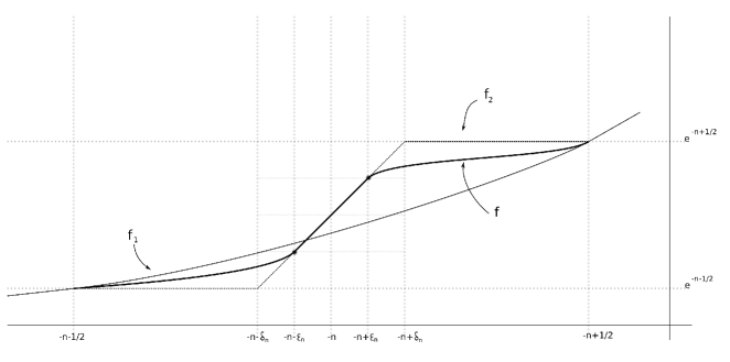
Figure 3.1. The function $f$

The following lemma is elementary, but for the convenience of the reader we include a proof.

Lemma 3.25.

For any $a,r>0$ the set $\mathcal{F}(a,r)$ is non-empty and path-connected. If $a^{\prime}\leq a$ and $r^{\prime}\geq r$ then $\mathcal{F}(a^{\prime},r^{\prime})\subseteq\mathcal{F}(a,r)$.

Proof.

We have already proved that $\mathcal{F}(a,r)$ is non-empty (see Remark 3.24 above). To show that $\mathcal{F}(a,r)$ is path-connected, first observe that if $f_{0},f_{1}\in\mathcal{F}(a,r)$ both satisfy (3.6) with the same constant $A>0$ then the linear homotopy $f_{s}:=sf_{1}+(1-s)f_{0}$ is contained in $\mathcal{F}(a,r)$ for all $s\in[0,1]$. It therefore suffices to show that if $f\in\mathcal{F}(a,r)$ satisfies (3.6) with respect to some $A>0$, then given any $B>A$ we can find a new function $f_{1}\in\mathcal{F}(a,r)$ that satisfies (3.6) with respect to $B$, and such that we may find a homotopy $(f_{s})_{s\in[0,1]}\subseteq\mathcal{F}(a,r)$ with $f_{0}=f$.

In order to do this, let $(\lambda_{s})_{s\in[0,1]}$ denote a family of smooth functions $\lambda_{s}:\mathbb{R}\rightarrow\mathbb{R}$ such that::

$$\lambda_{s}(\eta)=\begin{cases}\eta,&0\leq\eta<\infty,\\ \eta+s(B-A),&-\infty\leq\eta\leq-sB;\end{cases}\ \ \ 0<\lambda_{s}^{\prime}\leq 1$$

(such functions $\lambda_{s}$ exist as $A<B$). Set $f_{s}:=f\circ\lambda_{s}$. We claim that $f_{s}\in\mathcal{F}(a,r)$ for each $s\in[0,1]$. It is clear that $f_{s}\in\mathcal{F}(a)$ for each $s\in[0,1]$. Moreover,

$$(A+s(B-A))f_{s}^{\prime}(-A-s(B-A))=(A+s(B-A))f^{\prime}(-A)\geq Af^{\prime}(-A)>r.$$

Thus $f_{s}$ satisfies (3.6) with respect to $A+s(B-A)$ for each $s\in[0,1]$. The last statement of the lemma is immediate, and hence this completes the proof. ∎

The next result uses the same idea as [18, Proposition 5.5], and shows that for a suitable choice of $f\in\mathcal{F}$ one can bound the $\eta$ component of gradient flow lines with action in a fixed interval.

Proposition 3.26.

Fix $F\in\mathcal{D}$ and $0<a<b<\infty$. Let $\rho,T>0$ be the constants associated to $F$ from Corollary 3.21. Let $f\in\mathcal{F}\left(\frac{a}{6},\frac{b-a}{\min\{\rho,a/4T\}}\right)$ and $H\in\mathcal{H}(a/2)$. Choose $\chi$ such that $\mathfrak{f}:=(F,f,\chi,H)\in\mathfrak{F}_{0}$ and choose $J\in\mathcal{J}$. There exists a constant $C_{\textrm{\emph{mult}}}>0$ depending only on $a,b,F$ and $f$, such that if $u=(x,\eta)\in\mathcal{M}^{(a,b)}(\nabla_{J}A_{\mathfrak{f}})$, then $\left\|\eta\right\|_{L^{\infty}}\leq C_{\textrm{\emph{mult}}}$.

Proof.

First note that

(3.7) $$\lim_{s\rightarrow\pm\infty}\eta(s)\geq\frac{a}{2}.$$

Indeed, this follows from the fact that by (3.4),

$$A_{\mathfrak{f}}(x_{\pm},\eta_{\pm})=f(\eta_{\pm})-\int_{0}^{1}\{\lambda(X_{H}(t,x_{\pm}))-H(t,x_{\pm})\}dt,$$

and hence

$$f(\eta_{\pm})\geq A_{\mathfrak{f}}(x_{\pm},\eta_{\pm})-\kappa(H)\geq\frac{a}{2}.$$

Since $f\in\mathcal{F}(a/6)$ one therefore has $\eta_{\pm}\geq a/2$.

It will be convenient to define

$$\rho_{1}:=\min\left\{\rho,\frac{a}{4T}\right\},$$

so that $f\in\mathcal{F}\left(\frac{a}{6},\frac{b-a}{\rho_{1}}\right)$. By definition of the set $\mathcal{F}\left(\frac{a}{6},\frac{b-a}{\rho_{1}}\right)$, there exists $A>0$ such that

(3.8) $$f^{\prime}(-A)A>\frac{b-a}{\rho_{1}}.$$

Fix $u\in\mathcal{M}^{(a,b)}(\nabla_{J}A_{\mathfrak{f}})$. Define a function $\sigma_{u}:\mathbb{R}\rightarrow[0,\infty)$ by

(3.9) $$\sigma_{u}(s):=\inf\left\{\sigma\geq 0\,:\,\left\|\nabla_{J}A_{\mathfrak{f}}(u(s+\sigma))\right\|_{J}\leq\rho_{1}f^{\prime}(\eta(s+\sigma))\right\};$$

$\sigma_{u}$ is well defined as $\lim_{s\rightarrow\infty}f^{\prime}(\eta(s))=1$ (from (3.7) and the fact that $f\in\mathcal{F}(a/6)$), and $\lim_{s\rightarrow\infty}\left\|\nabla_{J}A_{\mathfrak{f}}(u(s))\right\|_{J}=0$. Next define

$$i_{u}(s):=\inf_{s\leq r\leq s+\sigma_{u}(s)}f^{\prime}(\eta(r)).$$

Note that

$$E(u)=\int_{-\infty}^{\infty}\left\|\nabla_{J}A_{\mathfrak{f}}(u(s))\right\|_{J}^{2}ds=\lim_{s\rightarrow-\infty}A_{\mathfrak{f}}(u(s))-\lim_{s\rightarrow\infty}A_{\mathfrak{f}}(u(s))\leq b-a.$$

Next,

$$E(u) \geq\int_{s}^{s+\sigma_{u}(s)}\left\|\nabla_{J}A_{\mathfrak{f}}(u(r))\right\|_{J}^{2}dr$$

$$\geq\int_{s}^{s+\sigma_{u}(s)}\rho_{1}^{2}f^{\prime}(\eta(r))^{2}dr$$

$$\geq\rho_{1}^{2}i_{u}(s)^{2}\sigma_{u}(s),$$

and hence

(3.10) $$\sigma_{u}(s)\leq\frac{b-a}{\rho_{1}^{2}i_{u}(s)^{2}}.$$

Now observe that

$$\left|\eta(s)-\eta(s+\sigma_{u}(s))\right| \leq\int_{s}^{s+\sigma_{u}(s)}\left|\partial_{r}\eta(r)\right|dr$$

$$\leq\left(\sigma_{u}(s)\int_{s}^{s+\sigma_{u}(s)}\left|\partial_{r}\eta(r)\right|^{2}dr\right)^{1/2}$$

$$\leq\left(\sigma_{u}(s)\int_{s}^{s+\sigma_{u}(s)}\left\|\nabla_{J}A_{\mathfrak{f}}(u(r))\right\|_{J}^{2}dr\right)^{1/2}$$

$$\leq(\sigma_{u}(s)E(u))^{1/2}$$

$$\leq\frac{b-a}{\rho_{1}i_{u}(s)},$$

where the last line used (3.10). Next, Corollary 3.21 implies that for any $s\in\mathbb{R}$,

$$f(\eta(s+\sigma_{u}(s)) \geq\frac{2}{3}\left(A_{\mathfrak{f}}(u(s+\sigma_{u}(s)))-T\left\|\nabla_{J}A_{\mathfrak{f}}(u(s+\sigma_{u}(s)))\right\|_{J}-\kappa(H)\right)$$

$$\geq\frac{2}{3}\left(a-T\rho_{1}f^{\prime}(\eta(s+\sigma_{u}(s)))-\frac{a}{2}\right).$$

Since $\rho_{1}\leq a/4T$ and $f^{\prime}\leq 1$, we deduce that

$$f(\eta(s+\sigma_{u}(s))\geq\frac{a}{6}.$$

Since $f\in\mathcal{F}(a/6)$ we see that

$$\eta(s+\sigma_{u}(s))\geq\frac{a}{6}>0,$$

and thus

$$\eta(s)\geq\frac{a}{6}-\frac{b-a}{\rho_{1}i_{u}(s)}>-\frac{b-a}{\rho_{1}i_{u}(s)}.$$

In particular,

$$f^{\prime}(\eta(s))\eta(s)\geq i_{u}(s)\eta(s)>-\frac{(b-a)}{\rho_{1}}.$$

Using (3.7), if there exists some $s_{0}\in\mathbb{R}$ such that $\eta(s_{0})<-A$ then by continuity there exists $s_{1}\in\mathbb{R}$ such that $\eta(s_{1})=-A$. But then we obtain a contradiction via (3.8)

$$-\frac{b-a}{\rho_{1}}>-f^{\prime}(-A)A=f^{\prime}(\eta(s_{1}))\eta(s_{1})>-\frac{b-a}{\rho_{1}}.$$

It follows that $\eta(s)>-A$ for all $s\in\mathbb{R}$.

Now we address the upper bound. Define a new function $\widetilde{\sigma}_{u}:\mathbb{R}\rightarrow[0,\infty)$ by

(3.11) $$\widetilde{\sigma}_{u}(s):=\inf\left\{\sigma\geq 0\,:\,\left\|\nabla_{J}A_{\mathfrak{f}}(u(s+\sigma))\right\|_{J}\leq\rho_{1}f^{\prime}(-A)\right\}.$$

Arguing as above we see that for any $s\in\mathbb{R}$,

$$\widetilde{\sigma}_{u}(s)\leq\frac{b-a}{\rho_{1}^{2}f^{\prime}(-A)^{2}},$$

and hence

(3.12) $$\left|\eta(s)-\eta(s+\widetilde{\sigma}_{u}(s))\right|\leq\frac{b-a}{\rho_{1}f^{\prime}(-A)}<A,$$

where the last inequality used (3.8) again. Then by Corollary 3.21 we see that for any $s\in\mathbb{R}$,

$$f(\eta(s+\widetilde{\sigma}_{u}(s)) \leq 2\left(A_{\mathfrak{f}}(u(s+\widetilde{\sigma}_{u}(s)))+T\left\|\nabla_{J}A_{\mathfrak{f}}(u(s+\widetilde{\sigma}_{u}(s)))\right\|_{J}+\kappa(H)\right)$$

$$\leq 2(b+T\rho_{1}f^{\prime}(-A)+a/2)\leq 2a+2b,$$

and hence $\eta(s+\widetilde{\sigma}_{u}(s))\leq 2a+2b$. Thus by (3.12),

$$\eta(s)<2a+2b+A.$$

We conclude that

$$\sup_{s\in\mathbb{R}}\left|\eta(s)\right|<C_{\textrm{mult}}=C_{\textrm{mult}}(a,b,f):=2a+2b+A.$$

∎

Proposition 3.26 prompts the following definition.

Definition 3.27.

Given $F\in\mathcal{D}$ and $0<a<b<\infty$, let

$$\mathcal{F}(F,a,b):=\mathcal{F}\left(\frac{a}{6},\frac{b-a}{\rho_{1}}\right),$$

where $\rho_{1}=\min\{\rho,a/4T\}$ and $\rho=\rho(F)$ and $T=T(F)$ are the constants from Corollary 3.21.

The following result is the main one of this section.

Theorem 3.28.

Fix $\alpha\in[S^{1},M]$. Suppose $\mathfrak{f}=(F,f,\chi,H)\in\mathfrak{F}_{0,\textrm{\emph{reg}}}$ and $0<a<b<\infty$ are such that $a,b\notin\mathcal{A}(A_{\mathfrak{f}},\alpha)$. Suppose also that $f\in\mathcal{F}(F,a,b)$ where $F\in\mathcal{D}(\Sigma)$, and $H\in\mathcal{H}(a/2)$. Let $S$ denote a fibrewise starshaped hypersurface such that $D(\Sigma)\subseteq D^{\circ}(S)$ and such that $\mbox{\emph{supp}}(X_{F})\subseteq D^{\circ}(S)$. Choose $J\in\mathcal{J}_{\textrm{\emph{reg}}}(\mathfrak{f})\cap\mathcal{J}(S)$. Then the quadruple $\mathfrak{q}:=(\mathfrak{f},a,b,J)$ is $\alpha$-admissible.

Proof.

Immediate from Corollary 3.11, Lemma 3.16 and Proposition 3.26.∎

Remark 3.29.

In fact, one can show using an argument based on Floer’s bifurcation method (see [18, Proposition 4.11]) that in the situation above, $HF^{(a,b)}(A_{F^{\chi},f}^{H},\alpha)$ is actually independent of the choice of $f\in\mathcal{F}(F,a,b)$. Nevertheless, for the purposes of the present paper we do not need this observation, and we will make no use of it.

3.4. Truncating the function $f$

  

A posteriori, we discover that one can truncate the function $f$ at infinity without affecting the Floer homology. Indeed, fix $\alpha\in[S^{1},M]$ and a non-degenerate fibrewise starshaped hypersurface $\Sigma$ and $0<a<b<\infty$ such that $a,b\notin\mathcal{A}(\Sigma,\alpha)$. Choose $F\in\mathcal{D}(\Sigma)$, $f\in\mathcal{F}(F,a,b)$ and $\chi\in\mathcal{X}$. Set $\mathfrak{f}:=(F,f,\chi,0)\in\mathfrak{F}_{0,\textrm{reg}}^{\prime}$. Suppose $R>2a+2b+A+1$, where $A>0$ is the constant associated to $f$ from (3.6). Let $\bar{f}:\mathbb{R}\rightarrow\mathbb{R}^{+}$ denote a smooth function such that $\bar{f}\equiv f$ on $(-\infty,R-1]$ and such that $\bar{f}(\eta)=R$ for $\eta\in[R+1,\infty)$, with $0\leq\bar{f}^{\prime}(\eta)\leq 1$ on all of $\mathbb{R}$. We will call such a function $\bar{f}$ an $R$-truncation of $f$. Let $\bar{\mathfrak{f}}:=(F,\bar{f},\chi,0)$.

Consider the Rabinowitz action functional $A_{\bar{\mathfrak{f}}}$. This functional will have many more critical points than $A_{\mathfrak{f}}$, as $\bar{f}^{\prime}$ is no longer strictly positive everywhere (i.e. one can no longer deduce (3.2) from (3.1)). However if $(x,\eta)$ is a critical point of $A_{\bar{\mathfrak{f}}}$ with $\bar{f}^{\prime}(\eta)=0$ then we necessarily have $\eta\geq R-1$, and hence $A_{\bar{\mathfrak{f}}}(x,\eta)=\bar{f}(\eta)\geq R-1$ by Lemma 3.6.1. In particular, $(x,\eta)\notin\mbox{Crit}^{(a,b)}(A_{\bar{\mathfrak{f}}})$. We conclude that

$$\mbox{Crit}^{(a,b)}(A_{\bar{\mathfrak{f}}},\alpha)=\mbox{Crit}^{(a,b)}(A_{\mathfrak{f}},\alpha).$$

In particular, this implies the Rabinowitz Floer complexes $CF^{(a,b)}(A_{\bar{\mathfrak{f}}},\alpha)$ and $CF^{(a,b)}(A_{\mathfrak{f}},\alpha)$ coincide as groups. Moreover the proof of Proposition 3.26 shows that the $\eta$-component of a gradient flow line $u=(x,\eta)\in\mathcal{M}^{(a,b)}(\nabla_{J}A_{\bar{\mathfrak{f}}})$ never escapes the interval $(-A,2a+2b+A]$ (for any $J\in\mathcal{J}$). In particular, $\eta$ never escapes $(-\infty,R-1)$. Since $f\equiv\bar{f}$ on $(-\infty,R-1]$, it follows that the differential of the two Floer complexes (with respect to a suitably chosen almost complex structure) is also the same, whence it follows that

$$HF^{(a,b)}(A_{\bar{\mathfrak{f}}},\alpha)\cong HF^{(a,b)}(A_{\mathfrak{f}},\alpha).$$

We will use this observation in the proof of Lemma 4.4 below.

3.5. Inclusion/Quotient maps

  

Let us make the following observation. Suppose we are given $a,b,c,d>0$ such that $a<\min\{b,c\}$ and $d>\max\{b,c\}$. Fix $\alpha\in[S^{1},M]$. Suppose $\Sigma$ is a non-degenerate fibrewise starshaped hypersurface and $F\in\mathcal{D}(\Sigma)$, and suppose that $a,b,c,d\notin\mathcal{A}(\Sigma,\alpha)$ and $f\in\mathcal{F}(F,a,d)$. Choose $\chi\in\mathcal{X}$ and $H\in\mathcal{H}(a/2)$ such that $\mathfrak{f}=(F,f,\chi,H)\in\mathfrak{F}_{0,\textrm{reg}}$. Fix an almost complex structure $J\in\mathcal{J}_{\textrm{ref}}(\mathfrak{f})\cap\mathcal{J}(S)$, where $S$ is a fibrewise starshaped hypersurface such that $D(\Sigma)\subseteq D^{\circ}(S)$. Our hypotheses imply that the three Floer homology groups

$$HF^{(a,b)}(A_{\mathfrak{f}},\alpha),\ HF^{(a,d)}(A_{\mathfrak{f}},\alpha)\ \mbox{and }HF^{(c,d)}(A_{\mathfrak{f}},\alpha)$$

are all well defined. There are natural chain maps between the three groups given by

$$CF^{(a,b)}(A_{\mathfrak{f}_{i}},\alpha)\overset{\textrm{inclusion}}{\rightarrow}CF^{(a,d)}(A_{\mathfrak{f}_{i}},\alpha)$$

and

$$CF^{(a,d)}(A_{\mathfrak{f}_{i}},\alpha)\overset{\textrm{quotient}}{\rightarrow}CF^{(a,d)}(A_{\mathfrak{f}_{i}},\alpha)/CF^{(a,c)}(A_{\mathfrak{f}_{i}},\alpha)=CF^{(c,d)}(A_{\mathfrak{f}_{i}},\alpha).$$

We denote by

(3.13) $$i:HF^{(a,b)}(A_{\mathfrak{f}},\alpha)\rightarrow HF^{(c,d)}(A_{\mathfrak{f}},\alpha)$$

the induced map on homology given by the composition of these two maps. It is clear that if

$$\mathcal{A}(\Sigma,\alpha)\cap[a,c]=\mathcal{A}(\Sigma,\alpha)\cap[b,d]=\emptyset$$

then $i$ is an isomorphism.

3.6. The Floer homology groups $HF^{(a,\infty)}(A_{F,f},\alpha)$

  

In this section we extend the definition of $HF^{(a,b)}$ to cover the case $b=\infty$. Suppose $\Sigma\subseteq T^{*}M$ is a non-degenerate fibrewise starshaped hypersurface. From this moment on it will be convenient to work with just one function $f$, instead of picking a function $f$ for each action interval $(a,b)$. For this purpose, set $\ell:=\ell(\Sigma)$ and choose

(3.14) $$f\in\bigcap_{r>0}\mathcal{F}(\ell/12,r)$$

(such functions exist by Remark 3.24). This function $f$ has the desirable property that given any $F\in\mathcal{D}(\Sigma)$ and any $\ell/2<a<b<\infty$ we have $f\in\mathcal{F}(F,a,b)$.

Fix $F\in\mathcal{D}(\Sigma)$ and $\alpha\in[S^{1},M]$. Then for any $\ell/2<a<b<\infty$ such that $a,b\notin\mathcal{A}(\Sigma,\alpha)$, the Floer homology $HF^{(a,b)}(A_{F,f},\alpha)$ is defined. Moreover if $c>b$ also satisfies $c\notin\mathcal{A}(\Sigma,\alpha)$, then from Section 3.5 there is a natural map $HF^{(a,b)}(A_{F,f},\alpha)\rightarrow HF^{(a,c)}(A_{F,f},\alpha)$. These maps form a directed system, and hence we can define

$$HF^{(a,\infty)}(A_{F,f},\alpha):=\underset{b\rightarrow\infty}{\underrightarrow{\lim}}HF^{(a,b)}(A_{F,f},\alpha).$$

We denote by

(3.15) $$\iota_{a}^{b}:HF^{(a,b)}(A_{F,f},\alpha)\rightarrow HF^{(a,\infty)}(A_{F,f},\alpha)$$

the induced map. Since we also have natural maps $HF^{(a,c)}(A_{F,f},\alpha)\rightarrow HF^{(b,c)}(A_{F,f},\alpha)$, there is an induced map

$$\pi_{a}^{b}:HF^{(a,\infty)}(A_{F,f},\alpha)\rightarrow HF^{(a,b)}(A_{F,f},\alpha).$$

For future use, given $3\ell/4<a<b<\infty$ with $a,b\notin\mathcal{A}(\Sigma,\alpha)$ let us denote by

$$Z(a,b):=\pi_{3\ell/4}^{b}\circ\iota_{3\ell/4}^{a},$$

so that $Z(a,b)$ is a map

(3.16) $$Z(a,b):HF^{(3\ell/4,a)}(A_{F,f},\alpha)\rightarrow HF^{(b,\infty)}(A_{F,f},\alpha).$$

Note that $Z(a,b)=0$ if $a<b$.

4. Continuation homomorphisms

In this section we develop the theory of continuation homomorphisms for the Rabinowitz action functional $A_{\mathfrak{f}}$. Continuation homomorphisms in Floer theory were introduced originally by Floer in [26], and are a powerful tool for proving invariance results for Floer homology. The main reason for introducing the function $f$ is that, as we will see below, these Floer homology groups behave well with respect to monotone homotopies. This is in contrast to the usual Rabinowitz Floer homology groups (see for instance [17]), for which it is not known whether they behave well with respect to monotone homotopies, see Remark 4.3 below.

4.1. Continuation maps

  

We begin with a discussion of continuation maps in the most general form that we will need. From now on we will be somewhat sloppy in our treatment of almost complex structures; wherever possible we will suppress them from the notation and from our discussion. Sometimes however we will be forced to include them in our notation (see for instance (4.1) below). In general the reader should think of $(J_{s})_{s\in[0,1]}$ as a generically chosen family of almost complex structures that all lie in $\mathcal{J}(S)$ for some fixed large fibrewise starshaped hypersurface $S$. We will not specify precisely what conditions $(J_{s})$ must satisfy, and will content ourselves with merely stating that these conditions are generically satisfied. In keeping with our new policy of supressing the mention of $J$, from now on we will refer to a triple $(\mathfrak{f},a,b)$ as being admissible if $(\mathfrak{f},a,b,J)$ is admissible (in the sense of Definition 3.17).

Suppose we are given a smooth family $\mathfrak{f}_{s}=(F_{s},f_{s},\chi_{s},H_{s})\subseteq\mathfrak{F}_{0}$ for $s\in[0,1]$. Assume that $\mathfrak{f}_{0}$ and $\mathfrak{f}_{1}$ lie in $\mathfrak{F}_{0,\textrm{reg}}$. Let us fix once and for all a smooth cut-off function $\beta:\mathbb{R}\rightarrow[0,1]$ such that $\beta(s)=0$ for $s\leq 0$ and $\beta(s)=1$ for $s\geq 1$, and $0\leq\beta^{\prime}(s)\leq 2$ for all $s\in\mathbb{R}$. Let $\mathcal{N}(\nabla A_{\mathfrak{f}_{s}},\alpha)$ denote the set of maps $u=(x,\eta):\mathbb{R}\rightarrow\Lambda_{\alpha}T^{*}M\times\mathbb{R}$ that satisfy

$$\partial_{s}u+\nabla_{J_{\beta(s)}}A_{\mathfrak{f}_{\beta(s)}}(u)=0.$$

It would be more accurate to write $\mathcal{N}(\nabla_{J_{\beta(s)}}A_{\mathfrak{f}_{\beta(s)}},\alpha)$, but we omit the “$J_{s}$” and the “$\beta$” in order to make the notation slightly less cumbersome. Thus $\mathcal{N}(\nabla A_{\mathfrak{f}_{s}},\alpha)$ is the set of maps $u=(x,\eta):\mathbb{R}\rightarrow\Lambda_{\alpha}T^{*}M\times\mathbb{R}$ that satisfy:

(4.1) $$\begin{cases}\partial_{s}x+J_{\beta(s),t}(x)(\partial_{t}x-f_{\beta(s)}(\eta)\chi_{\beta(s)}(t)X_{F_{\beta(s)}}(x)+X_{H_{\beta(s)}}(t,x))=0\\ \partial_{s}\eta-f_{\beta(s)}^{\prime}(\eta(s))\int_{0}^{1}F_{\beta(s)}(x)dt=0.\end{cases}$$

If $u=(x,\eta)$ satisfies (4.1) and has finite energy $E(u)<\infty$ then as before the limits

(4.2) $$\lim_{s\rightarrow\pm\infty}u(s,t)=:v_{\pm}(t)=(x_{\pm}(t),\eta_{\pm}),\ \ \ \lim_{s\rightarrow\pm\infty}\partial_{s}u(s,t)=0$$

exist and are uniform in the $t$-variable. Moreover $v_{-}\in\mbox{Crit}(A_{\mathfrak{f}_{0}},\alpha)$ and $v_{+}\in\mbox{Crit}(A_{\mathfrak{f}_{1}},\alpha)$.

Given $u\in\mathcal{N}(\nabla A_{\mathfrak{f}_{s}},\alpha)$ and $-\infty\leq s_{0}\leq s_{1}\leq\infty$, set

$$\Delta_{s_{0}}^{s_{1}}(u):=\int_{s_{0}}^{s_{1}}\left(\frac{\partial}{\partial s}A_{\mathfrak{f}_{\beta(s)}}\right)(u(s))ds.$$

Write $\Delta(u):=\Delta_{-\infty}^{\infty}(u)$. Following Ginzburg [30], given $C\geq 0$ let us say the family $(\mathfrak{f}_{s})$ is $C$-bounded if for every $u\in\mathcal{N}(\nabla A_{\mathfrak{f}_{s}},\alpha)$ and every $-\infty\leq s_{0}\leq s_{1}\leq\infty$ it holds that

$$\Delta_{s_{0}}^{s_{1}}(u)\leq C.$$

In order to explain the relevance of the term $\Delta_{s_{0}}^{s_{1}}(u)$, given $a,b>0$ denote by $\mathcal{N}_{a}^{b}(\nabla A_{\mathfrak{f}_{s}},\alpha)$ the subset of $\mathcal{N}(\nabla A_{\mathfrak{f}_{s}},\alpha)$ consisting of those maps $u$ that satisfy

$$\lim_{s\rightarrow-\infty}A_{\mathfrak{f}_{\beta(s)}}(u(s))\leq b,\ \ \ \lim_{s\rightarrow\infty}A_{\mathfrak{f}_{\beta(s)}}(u(s))\geq a.$$

Then if $u\in\mathcal{N}_{a}^{b}(\nabla A_{\mathfrak{f}_{s}},\alpha)$ one readily checks that

(4.3) $$E(u)\leq b-a+\Delta(u);$$

(4.4) $$\sup_{s\in\mathbb{R}}A_{\mathfrak{f}_{\beta(s)}}(u(s))\leq b+\sup_{s\in\mathbb{R}}\Delta_{-\infty}^{s}(u);$$

(4.5) $$\inf_{s\in\mathbb{R}}A_{\mathfrak{f}_{\beta(s)}}(u(s))\geq a-\sup_{s\in\mathbb{R}}\Delta_{s}^{\infty}(u).$$

In particular,

$$\lim_{s\rightarrow\infty}A_{\mathfrak{f}_{\beta(s)}}(u(s))\leq b+\Delta(u);$$

$$\lim_{s\rightarrow\infty}A_{\mathfrak{f}_{\beta(s))}}(u(s))\geq a-\Delta(u).$$

Definition 4.1.

Fix a family $(\mathfrak{f}_{s})_{s\in[0,1]}$ as above, and fix $a,b>0$ and $C\geq 0$. We say that $\{(\mathfrak{f}_{s}),a,b,C\}$ is an $\alpha$-admissible family if

1. The triples $(\mathfrak{f}_{0},a,b)$ and $(\mathfrak{f}_{1},a+C,b+C)$ are $\alpha$-admissible. Thus $HF^{(a,b)}(A_{\mathfrak{f}_{0}},\alpha)$ and $HF^{(a+C,b+C)}(A_{\mathfrak{f}_{1}},\alpha)$ are well defined.

2. The family $(\mathfrak{f}_{s})$ is $C$-bounded.

3. There exist constants $C_{\textrm{loop}},C_{\textrm{mult}}>0$ such that if $u=(x,\eta)\in\mathcal{N}_{a}^{b}(\nabla A_{\mathfrak{f}_{s}},\alpha)$ then it holds that $\left\|x\right\|_{L^{\infty}}<C_{\textrm{loop}}$ and $\left\|\eta\right\|_{L^{\infty}}<C_{\textrm{mult}}$.

The following basic theorem follows from standard Floer homological methods; see for instance [15, Section 4.4] or [30, Section 3.2.3].

Theorem 4.2.

(Continuity properties of filtered Floer homology)

1. Suppose $\{(\mathfrak{f}_{s}),a,b,C\}$ is an $\alpha$-admissible family. Then there exists a chain map

   $$\Psi:CF^{(a,b)}(A_{\mathfrak{f}_{0}},\alpha)\rightarrow CF^{(a+C,b+C)}(A_{\mathfrak{f}_{1}},\alpha)$$

   which induces a homomorphism

   $$\psi:HF^{(a,b)}(A_{\mathfrak{f}_{0}},\alpha)\rightarrow HF^{(a+C,b+C)}(A_{\mathfrak{f}_{1}},\alpha).$$

2. Suppose $c,d>0$ are such that $a\leq c$ and $b\leq d$. Suppose in addition that $\{(\mathfrak{f}_{s}),c,d,C\}$ is $\alpha$-admissible. Then the following diagram commutes:

   Here the vertical maps are the maps from (3.13).

4.2. Monotone homotopies

  

In this section we suppose we are given two non-degenerate fibrewise starshaped hypersurfaces $\Sigma$ and $\Sigma^{\prime}$ with the property that

$$D(\Sigma^{\prime})\subseteq D(\Sigma).$$

Let us first fix a smooth family $(\Sigma_{s})_{s\in[0,1]}$ of fibrewise starshaped hypersurfaces such that:

1. $\Sigma_{0}=\Sigma$ and $\Sigma_{1}=\Sigma^{\prime}$;

2. For generic $s\in[0,1]$, $\Sigma_{s}$ is non-degenerate;

3. for any $0\leq s_{0}\leq s_{1}\leq 1$ one has $D(\Sigma_{s_{1}})\subseteq D(\Sigma_{s_{0}})$.

We will call such a family a concentric family of fibrewise starshaped hypersurfaces. Given such a family $(\Sigma_{s})$ it is possible to choose a smooth family $(F_{s})_{s\in[0,1]}\subseteq\mathcal{D}$ of Hamiltonians such that $F_{s}\in\mathcal{D}(\Sigma_{s})$ and such that $\partial_{s}F_{s}(q,p)\geq 0$ for all $(q,p)\in T^{*}M$. For the remainder of this section we fix such a family $(F_{s})$.

Set

$$\ell:=\min_{s\in[0,1]}\ell(\Sigma_{s})>0,$$

and fix once and for all a function $f\in\bigcap_{r>0}\mathcal{F}\left(\ell/12,r\right)$. By construction, given any $s\in[0,1]$ such that $\Sigma_{s}$ is non-degenerate, and any $\alpha\in[S^{1},M]$, $\chi\in\mathcal{X}$, and $\ell/2<a<b<\infty$ such that $\mathcal{A}(\Sigma_{s},\alpha)\cap\{a,b\}=\emptyset$, the Floer homology $HF^{(a,b)}(A_{F_{s}^{\chi},f},\alpha)$ is well defined. In this section we will only ever use $\chi\equiv 1$, so let us set

$$\mathfrak{f}_{s}:=(F_{s},f,1,0).$$

Now let us fix $\alpha\in[S^{1},M]$. Suppose we are given $\ell/2<a<b<\infty$ such that $a,b\notin\mathcal{A}(\Sigma,\alpha)\cup\mathcal{A}(\Sigma^{\prime},\alpha)$. Then we claim there exists a chain map

$$\Psi_{0}^{1}:CF^{(a,b)}(A_{\mathfrak{f}_{0}},\alpha)\rightarrow CF^{(a,b)}(A_{\mathfrak{f}_{1}},\alpha)$$

inducing a homomorphism

$$\psi_{0}^{1}:HF^{(a,b)}(A_{\mathfrak{f}_{0}},\alpha)\rightarrow HF^{(a,b)}(A_{\mathfrak{f}_{1}},\alpha).$$

This follows readily from our discussion above. Indeed, we claim that $\{(\mathfrak{f}_{s}),a,b,0\}$ is an $\alpha$-admissible family. Condition (1) of Definition 4.1 is satisfied by assumption, and since $\partial_{s}F_{s}\geq 0$ we have $\Delta_{s_{0}}^{s_{1}}(u)\leq 0$ for all $u\in\mathcal{N}(\nabla A_{\mathfrak{f}_{s}},\alpha)$ and $-\infty\leq s_{0}\leq s_{1}\leq\infty$, which shows Condition (2) is satisfied.

Remark 4.3.

The innocent looking fact that $\partial_{s}F_{s}\geq 0$ implies $\Delta_{s_{0}}^{s_{1}}(u)\leq 0$ is in fact the key point of the present paper, and the whole point of perturbing the Rabinowitz action functional with a positive function $f$. In the setting of ’standard’ Rabinowitz Floer homology, the corresponding expression for $\Delta_{s_{0}}^{s_{1}}(u)$ is given by $-\int_{s_{0}}^{s_{1}}\eta(s)\int_{0}^{1}\partial_{s}F_{\beta(s)}(x(s))ds$ instead of $-\int_{s_{0}}^{s_{1}}f(\eta(s))\int_{0}^{1}\partial_{s}F_{\beta(s)}(x(s))ds$. Since the Lagrange multiplier $\eta(s)$ could very well become negative, one cannot conclude from $\partial_{s}F_{s}\geq 0$ that $\Delta_{s_{0}}^{s_{1}}(u)\leq 0$ in the standard case.

The existence of a constant $C_{\textrm{loop}}>0$ satisfying the requirements of Condition (3) follows from the choice of a correct almost complex structure, and we will say nothing about this (see the opening paragraph of Section 4). Equations (4.3), (4.4) and (4.5) show that the proof of Proposition 3.26 goes through without change to establish the existence of a constant $C_{\textrm{mult}}>0$ such that Condition (3) of Definition 4.1 is satisfied. Thus theorem 4.2 proves the claim.

Note that there is nothing special about $s=0$ and $s=1$; in general given any $0\leq s_{0}\leq s_{1}\leq 1$ such that $\Sigma_{s_{0}}$ and $\Sigma_{s_{1}}$ are non-degenerate and $a,b\notin\mathcal{A}(\Sigma_{s_{0}},\alpha)\cup\mathcal{A}(\Sigma_{s_{1}},\alpha)$, this construction gives a map

$$\Psi_{s_{0}}^{s_{1}}:CF^{(a,b)}(A_{\mathfrak{f}_{s_{0}}},\alpha)\rightarrow CF^{(a,b)}(A_{\mathfrak{f}_{s_{1}}},\alpha)$$

inducing a map

$$\psi_{s_{0}}^{s_{1}}:HF^{(a,b)}(A_{\mathfrak{f}_{s_{0}}},\alpha)\rightarrow HF^{(a,b)}(A_{\mathfrak{f}_{s_{1}}},\alpha)$$

In fact, we can say rather more about the homomorphisms $(\psi_{s_{0}}^{s_{1}})$. As with Theorem 4.2 itself, these two properties follow from standard Floer homological methods. See for instance [15, Section 4.4] or [30, Section 3.2.3].

1. Firstly, the maps $(\psi_{s_{0}}^{s_{1}})$ are actually independent of choice of $(\Sigma_{s})$ in the following sense. Suppose $(\widetilde{\Sigma}_{s})_{s\in[0,1]}$ is another family of fibrewise starshaped hypersurfaces satisfying the three conditions above, with corresponding definining Hamiltonians $(\widetilde{F}_{s})$. Let

   $$\widetilde{\ell}:=\min_{s\in[0,1]}\ell(\widetilde{\Sigma}_{s}).$$

   Suppose that $f\in\bigcap_{r>0}\mathcal{F}(\widetilde{\ell}/12,r)$. Set $\widetilde{\mathfrak{f}}_{s}:=(\widetilde{F}_{s},f,1,0)$. Then $\{(\widetilde{\mathfrak{f}}_{s}),a,b,0\}$ is also an $\alpha$-admissible family, and hence gives rise to another family of chain maps $(\widetilde{\Psi}_{s_{0}}^{s_{1}})$. These chain maps are chain homotopic to the original chain maps, and hence they induce the same map on homology.

2. The induced maps $(\psi_{s_{0}}^{s_{1}})$ enjoy the following functorial properties whenever they are defined:

   $$\psi_{s_{0}}^{s_{2}}=\psi_{s_{1}}^{s_{2}}\circ\psi_{s_{0}}^{s_{1}}\ \ \ \mbox{whenever}\ \ \ 0\leq s_{0}\leq s_{1}\leq s_{2}\leq 1;$$

   $$\psi_{s_{0}}^{s_{0}}=\mathbb{1}.$$

The proof of the next lemma requires a little more work, but is by now standard.

Lemma 4.4.

Suppose in addition that $a,b\notin\mathcal{A}(\Sigma_{s},\alpha)$ for all $s\in[0,1]$. Then the homomorphism $\psi_{0}^{1}$ is actually an isomorphism.

Proof.

Let $\rho_{s},T_{s}>0$ be the constants for $F_{s}$ from Corollary 3.21 (note $\rho_{s}$ and $T_{s}$ depend continuously on $s$, cf. Remark 3.22). Let

$$\rho_{1}:=\min\left\{\min_{s}\rho_{s},\frac{a}{4\max_{s}T_{s}}\right\}.$$

Our choice of $f$ guarantees that there exists $0<\varepsilon<a/4$ and $A>0$ such that

(4.6) $$f(\eta)=\eta\ \ \ \mbox{for all }\eta\geq\frac{a-4\varepsilon}{6};$$

(4.7) $$Af^{\prime}(-A)>\frac{b-a+\varepsilon}{\rho_{1}}.$$

Shrinking $\varepsilon$ if necessary, we may assume in addition that

(4.8) $$\mathcal{A}(\Sigma_{s},\alpha)\cap[a,a+\varepsilon]=\mathcal{A}(\Sigma_{s},\alpha)\cap[b,b+\varepsilon]=\emptyset$$

for all $s\in[0,1]$. Now choose $R>2a+2b+A+1$ and let $\bar{f}$ denote an $R$-truncation of $f$ (see Section 3.4). Set $\mathfrak{g}_{s}:=(F_{1-s},\bar{f},1,0)$. Our choice of $R$ implies that for every $s\in[0,1]$ such that $\Sigma_{s}$ is non-degenerate, the Floer homology $HF^{(a,b)}(A_{\mathfrak{g}_{s}},\alpha)$ is well defined, and moreover

$$HF^{(a,b)}(A_{\mathfrak{f}_{0}},\alpha)\cong HF^{(a,b)}(A_{\mathfrak{g}_{1}},\alpha);$$

$$HF^{(a,b)}(A_{\mathfrak{f}_{1}},\alpha)\cong HF^{(a,b)}(A_{\mathfrak{g}_{0}},\alpha).$$

Now we compute that for $u\in\mathcal{N}(\nabla A_{\mathfrak{g}_{s}},\alpha)$ and $-\infty\leq s_{0}\leq s_{1}\leq\infty$,

$$\Delta_{s_{0}}^{s_{1}}(u)= -\int_{s_{0}}^{s_{1}}\bar{f}(\eta)\int_{0}^{1}\left(\partial_{s}F_{\beta(1-s)}(x)\right)dtds$$

$$\leq 2R\sup_{s\in[0,1]}\left\|\partial_{s}F_{s}\right\|_{\infty}.$$

Choose $N\in\mathbb{N}$ and a subdivision $0<i_{0}<i_{1}<\dots<i_{N}=1$ such that

(4.9) $$\max_{0\leq p\leq N-1}\left|i_{p+1}-i_{p}\right|\leq\frac{\varepsilon}{2R\sup_{s\in[0,1]}\left\|\partial_{s}F_{s}\right\|_{\infty}},$$

and such that $\Sigma_{i_{p}}$ is non-degenerate for each $p=0,1,\dots,N$. Now set

$$\mathfrak{g}_{s}^{p}:=\left(F_{(1-s)i_{p+1}-si_{p}},\bar{f},1,0\right).$$

We claim that $\{(\mathfrak{g}_{s}^{p}),a,b,\varepsilon\}$ is an $\alpha$-admissible family for each $p=0,1,\dots,N-1$. Indeed, Condition (1) of Definition 4.1 is obviously satisfied, and Condition (2) is satisfied by (4.9). Finally, the reader is invited to check that our two assumptions (4.6) and (4.7) together with the equations (4.3), (4.4) and (4.5) mean that the proof of Proposition 3.26 goes through to ensure that Condition (3) is satisfied for each $p=0,1,\dots,N-1$.

As a result, Theorem 4.2 implies that for each $p=0,1,\dots,N-1$ there exists a chain map

$$\Phi_{i_{p+1}}^{i_{p}}:CF^{(a,b)}(A_{\mathfrak{f}_{i_{p+1}}},\alpha)\rightarrow CF^{(a+\varepsilon,b+\varepsilon)}(A_{\mathfrak{f}_{i_{p}}},\alpha)$$

inducing a homomorphism

$$\phi_{i_{p+1}}^{i_{p}}:HF^{(a,b)}(A_{\mathfrak{f}_{i_{p+1}}},\alpha)\rightarrow HF^{(a+\varepsilon,b+\varepsilon)}(A_{\mathfrak{f}_{i_{p}}},\alpha).$$

Next, note that (4.8) and (3.13) imply that

$$i:HF^{(a,b)}(A_{\mathfrak{f}_{i_{p}}},\alpha)\cong HF^{(a+\varepsilon,b+\varepsilon)}(A_{\mathfrak{f}_{i_{p}}},\alpha)\ \ \ \mbox{for all }p=0,1,\dots,N,$$

and consequently we may think of $\phi_{i_{p+1}}^{i_{p}}$ as a map

$$\phi_{i_{p+1}}^{i_{p}}:HF^{(a,b)}(A_{\mathfrak{f}_{i_{p+1}}},\alpha)\rightarrow HF^{(a,b)}(A_{\mathfrak{f}_{i_{p}}},\alpha).$$

It is now easy to see from the two properties about the continuation maps given just before the statement of the lemma that $\phi_{i_{p+1}}^{i_{p}}$ is an isomorphism with inverse given by $\psi_{i_{p}}^{i_{p+1}}$. It thus follows that if

$$\phi_{1}^{0}:=\phi_{i_{N}}^{i_{N-1}}\circ\dots\circ\phi_{i_{2}}^{i_{1}}\circ\phi_{i_{1}}^{i_{0}},$$

then $\phi_{1}^{0}$ is the desired inverse to $\psi_{0}^{1}$. ∎

We will be interested in a slight generalization of this.

Proposition 4.5.

Suppose we are given two smooth strictly decreasing families $(a_{s})_{s\in[0,1]}$ and $(b_{s})_{s\in[0,1]}$ such that $\ell/2<a_{s}<b_{s}<\infty$ for all $s\in[0,1]$ and such that $a_{s},b_{s}\notin\mathcal{A}(\Sigma_{s},\alpha)$ for all $s\in[0,1]$. Then there exists a chain map

$$\Theta_{0}^{1}:CF^{(a_{0},b_{0})}(A_{\mathfrak{f}_{0}},\alpha)\rightarrow CF^{(a_{1},b_{1})}(A_{\mathfrak{f}_{1}},\alpha)$$

inducing an isomorphism

$$\theta_{0}^{1}:HF^{(a_{0},b_{0})}(A_{\mathfrak{f}_{0}},\alpha)\rightarrow HF^{(a_{1},b_{1})}(A_{\mathfrak{f}_{1}},\alpha).$$

Moreover the following diagram commutes:

where

$$i:HF^{(a_{1},b_{1})}(A_{\mathfrak{f}_{1}},\alpha)\rightarrow HF^{(a_{0},b_{0})}(A_{\mathfrak{f}_{`}},\alpha)$$

is the map from (3.13).

Proof.

The trick here is to use a “staircase” method to deal with the fact that the endpoints are changing. This is explained in detail in [41, p18], but the general idea is the following. There exists $N\in\mathbb{N}$ and sequences

$$0=i_{0}<i_{1}<\dots<i_{N}=1;$$

$$0=j_{0}<j_{1}<\dots<j_{N}=1;$$

$$0=k_{0}<k_{1}<\dots<k_{N}=1$$

such that for all $p\in\{0,1,\dots,N-1\}$, $\Sigma_{k_{p}}$ is non-degenerate and

(4.10) $$\mathcal{A}(\Sigma_{s},\alpha)\cap[a_{i_{p+1}},a_{i_{p}}]=\mathcal{A}(\Sigma_{s},\alpha)\cap[b_{j_{p+1}},b_{j_{p}}]=\emptyset\ \ \ \mbox{for all }s\in[k_{p},k_{p+1}].$$

We already know from the previous lemma how to build isomorphisms

$$\psi_{p}:HF^{(a_{i_{p}},b_{j_{p}})}(\Sigma_{k_{p}},\alpha)\rightarrow HF_{\mathcal{}}^{(a_{i_{p}},b_{j_{p}})}(\Sigma_{k_{p+1}},\alpha),$$

and (4.10) implies that

$$HF^{(a_{i_{p}},b_{i_{p}})}(\Sigma_{k_{p+1}},\alpha)\cong HF_{\mathcal{}}^{(a_{i_{p+1}},b_{j_{p+1}})}(\Sigma_{k_{p+1}},\alpha).$$

Thus we obtain isomorphisms

$$\theta_{p}:HF_{\mathcal{}}^{(a_{i_{p}},b_{j_{p}})}(\Sigma_{k_{p}},\alpha)\rightarrow HF^{(a_{i_{p+1}},b_{j_{p+1}})}(\Sigma_{k_{p+1}},\alpha),$$

and the proposition follows with

$$\theta_{0}^{1}:=\theta_{N-1}\circ\dots\circ\theta_{1}\circ\theta_{0}.$$

∎

4.3. Leaf-wise intersections

  

In this section we start with a single non-degenerate fibrewise starshaped hypersurface $\Sigma$. As before, set $\ell:=\ell(\Sigma)$ and fix once and for all a function $f\in\bigcap_{r>0}\mathcal{F}\left(\ell/12,r\right)$ and a defining Hamiltonian $F\in\mathcal{D}(\Sigma)$. Given a class $\alpha\in[S^{1},M]$ and a map $\varphi\in\mbox{Ham}_{c}(T^{*}M,\omega)$, let us denote by $n_{\Sigma,\alpha}(\varphi,(a,b))$ the number of positive leaf-wise intersections points of $\varphi$ in $\Sigma$ that belong to $\alpha$ and have time-shift $T\in(a,b)$. The following lemma explains the link between the Floer homology of a suitable perturbed Rabinowitz action functional $A_{F^{\chi},f}^{H}$ and the number of positive leaf-wise intersections of $\varphi$. The proof is immediate from Lemma 3.6.2 and Theorem 3.28.

Lemma 4.6.

Suppose $\varphi\in\mbox{\emph{Ham}}_{c}(T^{*}M,\omega)$ is generated by $H\in\mathcal{H}$. Choose $\chi\in\mathcal{X}_{0}$ and set $\mathfrak{f}:=(F,f,\chi,H)$. Fix $\ell/2<a<b<\infty$ such that $H\in\mathcal{H}(a/2)$ and $a,b\notin\mathcal{A}(A_{\mathfrak{f}},\alpha)$. If $\mathfrak{f}\in\mathfrak{F}_{0,\textrm{\emph{reg}}}^{\prime\prime}$ (which we can assume is the case for a generic $\varphi$) then $HF^{(a,b)}(A_{\mathfrak{f}},\alpha)$ is well defined. Moreover, provided $\varphi$ has no periodic leaf-wise intersection points (which again, we may assume is the case for a generic $\varphi$ by Proposition 3.8) one has

$$n_{\Sigma,\alpha}(\varphi,(a,b))\geq\dim\,HF^{(a,b)}(A_{\mathfrak{f}},\alpha).$$

Now set $\mathfrak{g}:=(F,f,\chi,0)$, and note that $\mathfrak{g}\in\mathfrak{F}_{0,\textrm{reg}}^{\prime}$. Our next application of continuation homomorphisms is to interpolate between the Floer homology of the perturbed Rabinowitz action functional $A_{\mathfrak{f}}$ and the non-perturbed one $A_{\mathfrak{g}}$. This lemma is a simple consequence of Theorem 4.2.

Lemma 4.7.

Assume in addition that

$$a-\left\|H\right\|_{-},a+\left\|H\right\|_{+},b-\left\|H\right\|_{-},b+\left\|H\right\|_{+}\notin\mathcal{A}(\Sigma,\alpha),$$

Thus both $HF^{(a-\left\|H\right\|_{-},b-\left\|H\right\|_{-})}(A_{\mathfrak{g}},\alpha)$ and $HF^{(a+\left\|H\right\|_{+},b+\left\|H\right\|_{+})}(A_{\mathfrak{g}},\alpha)$ are well defined. Assume moreover that not only is $H\in\mathcal{H}(a/2)$ but actually

(4.11) $$2\left\|H\right\|+\kappa(H)\leq\frac{a}{2}.$$

Then there exists a commutative diagram

Proof.

Let us first build the continuation map

(4.12) $$HF^{(a-\left\|H\right\|_{-},b-\left\|H\right\|_{-})}(A_{\mathfrak{g}},\alpha)\rightarrow HF^{(a,b)}(A_{\mathfrak{f}},\alpha).$$

Set

$$\mathfrak{f}_{s}:=(F,f,\chi,sH)\ \ \ \mbox{for }s\in[0,1].$$

We will verify that $\{(\mathfrak{f}_{s}),a-\left\|H\right\|_{-},b-\left\|H\right\|_{-},\left\|H\right\|_{-}\}$ forms an $\alpha$-admissible family in the sense of Definition 4.1. Condition (1) is satisfied by assumption. Suppose $u\in\mathcal{N}(\nabla A_{\mathfrak{f}_{s}},\alpha)$ and $-\infty\leq s_{0}\leq s_{1}\leq\infty$. This time we have

$$\Delta_{s_{0}}^{s_{1}}(u) =-\int_{s_{0}}^{s_{1}}\beta^{\prime}(s)\int_{0}^{1}H(t,x)dtds$$

$$\leq\int_{0}^{1}\beta^{\prime}(s)\left\|H\right\|_{-}ds$$

$$=\left\|H\right\|_{-}.$$

Thus Condition (2) is satisfied. The reader may check that the stronger assumption (4.11) implies that the proof of Proposition 3.26 goes through to provide the necessary constant $C_{\textrm{mult}}>0$ to satisfy Condition (3). The existence of the map (4.12) now follows from Theorem 4.2. The second map is defined similarly. ∎

Now set $\mathfrak{h}:=(F,f,1,0)$. We now want to interpolate between the Floer homology of $A_{\mathfrak{g}}$ and the Floer homology of $A_{\mathfrak{h}}$.

Lemma 4.8.

Suppose $\ell/2<a<b<\infty$ satisfy $a,b\notin\mathcal{A}(\Sigma,\alpha)$. Then there exists an isomorphsim

$$HF^{(a,b)}(A_{\mathfrak{g}},\alpha)\rightarrow HF^{(a,b)}(A_{\mathfrak{h}},\alpha).$$

This lemma is proved in a similar fashion (in fact it’s slightly easier) to the proof of Lemma 4.4, and as such we omit the proof. Putting the results of this section together we deduce:

Corollary 4.9.

Assume the hypotheses of Lemma 4.7. Then

$$n_{\Sigma,\alpha}(\varphi,(a,b))\geq\mbox{\emph{rank}}\left\{i:HF^{(a-\left\|H\right\|_{-},b-\left\|H\right\|_{-})}(A_{\mathfrak{h}},\alpha)\rightarrow HF^{(a+\left\|H\right\|_{+},b+\left\|H\right\|_{+})}(A_{\mathfrak{h}},\alpha)\right\}.$$

5. The convex case

5.1. $L^{\infty}$ estimates for Hamiltonians that are not constant outside a compact set

  

Throughout this section, assume $\Sigma\subseteq T^{*}M$ is a strictly fibrewise convex non-degenerate fibrewise starshaped hypersurface. By this we mean a fibrewise starshaped hypersurface with the additional property that for each $q\in M$ the hypersurface $\Sigma\cap T_{q}^{*}M$ in $T_{q}^{*}M$ has a positive definite second fundamental form. Let $\ell:=\ell(\Sigma)$, and fix once and for all a function $f\in\bigcap_{r>0}\mathcal{F}(\ell/12,r)$.

For each $q\in M$, let $r_{q}:T_{q}^{*}M\rightarrow\mathbb{R}$ denote the function that is homogeneous of degree $2$ and satisfies $r_{q}|_{\Sigma\cap T_{q}^{*}M}\equiv 1$. The function $(q,p)\mapsto r_{q}(p)$ is $C^{1}$ on all of $T^{*}M$, but not necessarily smooth at the zero section. In order to correct this, let $\rho:\mathbb{R}\rightarrow\mathbb{R}$ denote a smooth function such that $\rho(s)=0$ for $s\leq\varepsilon$, and $\rho^{\prime}(s)>0$ for $s>\varepsilon$, and $\rho(s)=s$ for $s\geq 2\varepsilon$, where $\varepsilon$ is some sufficiently small positive number. Then define $F:T^{*}M\rightarrow\mathbb{R}$ by

(5.1) $$F(q,p):=\frac{1}{2}(\rho(r_{q}(p))-1).$$

If $(q,p)\in\Sigma$ then

$$\lambda(X_{F}(q,p))=\omega(Y(q,p),X_{F}(q,p))=d_{(q,p)}F(Y(q,p))=r_{q}(p)=1.$$

Of course, the function $F$ is not compactly supported, and thus $F\notin\mathcal{D}(\Sigma)$, and hence $F$ cannot a priori be used to compute the $\mathcal{F}$-Rabinowitz Floer homology of $\Sigma$. In order to make it compactly supported, we truncate it at infinity. Given $R>1$, let $F_{R}:T^{*}M\rightarrow\mathbb{R}$ denote a function such that $F_{R}(q,p)=F(q,p)$ on $\{F\leq R-1\}$ and such that $F_{R}(q,p)=R$ on $\{F\geq R+1\}$. Then $F_{R}\in\mathcal{D}(\Sigma)$, and the aim of this section is to compute $HF^{(3\ell/4,\infty)}(A_{F_{R},f},\alpha)$ for each $\alpha\in[S^{1},M]$.

The following result is highly non-trivial, and is taken from [4, Section 3] (the function $f$ makes no difference here, given that we know a priori that the $\eta$-component of elements $u\in\mathcal{M}^{(a,b)}(\nabla_{J}A_{F_{R_{1}},f})$ are uniformly bounded).

Theorem 5.1.

Let $S$ denote a fibrewise starshaped hypersurface such that $D(\Sigma)\subseteq D^{\circ}(S)$ and such that $\mbox{\emph{supp}}(X_{F})\subseteq D^{\circ}(S)$. Choose $J\in\mathcal{J}(S)$. Choose $0<a<b<\infty$ such that $a,b\notin\mathcal{A}(\Sigma,\alpha)$. Then there exists $R_{1},R_{0}>1$ with $R_{1}>R_{0}+1$ such that if $u=(x,\eta)\in\mathcal{M}^{(a,b)}(\nabla_{J}A_{F_{R_{1}},f})$ then $x(\mathbb{R}\times S^{1})\subseteq\{F\leq R_{0}\}$.

In other words, as far as the gradient flow lines $u\in\mathcal{M}^{(a,b)}(\nabla_{J}A_{F,f})$ are concerned, we might as well not have truncated $F$ at all. This result is not obvious; although Lemma 3.16 implies that there certainly exists $R_{2}>0$ such that if $u=(x,\eta)\in\mathcal{M}^{(a,b)}(\nabla_{J}A_{F_{R_{1}},f})$ then $x(\mathbb{R}\times S^{1})\subseteq\{F\leq R_{2}\}$, there is absolutely no reason at all why we should have $R_{1}>R_{2}+1$. In order to prove this result, one must first show that one can obtain $L^{\infty}$ bounds for the Hamiltonian $F$ without first truncating it at infinity, and then show that these bounds are unaffected if we then subsequently truncate $F$ at some sufficiently large $R>0$. This last statement is only true because we restrict to the action interval $(a,b)$. In other words, this proves the Floer homology $HF^{(a,b)}(A_{F,f},\alpha)$ is well defined if we use the Hamiltonian $F$, and moreover with a little more work this shows that the Floer homology $HF^{(a,b)}(A_{F,f},\alpha)$ is isomorphic to Floer homology $HF^{(a,b)}(A_{F_{R},f},\alpha)$. An alternative proof of Theorem 5.1 is given in [43, Section 6]. Anyway, because of Theorem 5.1, we may as well work directly with the Hamiltonian $F$, rather than truncating it at infinity. This is crucial for Theorem 5.12 below.

5.2. The $f$-free time action functional

  

The Hamiltonian $F$ has positive definite fibrewise second differential, and thus the Fenchel transform $L:TM\rightarrow\mathbb{R}$ is well defined. Explicitly, $L$ is the unique Lagrangian on $TM$ defined by

$$L(q,v):=\max_{p\in T_{q}M}\left\{p(v)-F(q,p)\right\}.$$

The Legendre transformation associated to $L$ is the diffeomorphism $TM\cong T^{*}M$ given by $(q,v)\mapsto\left(q,\frac{\partial L}{\partial v}(q,v)\right)$. One can recover $F$ from $L$ via

$$F(q,p)=\frac{\partial L}{\partial v}(q,v)(v)-L(q,v)\ \ \ \mbox{where }\frac{\partial L}{\partial v}(q,v)=p.$$

Fix a Riemannian metric $g$ on $M$ for the remainder of this section. There exist constants $c_{0},c_{1}>0$ such that for all $(q,v)\in TM$,

(5.2) $$d_{v}^{2}(L|_{T_{q}M})\geq c_{0}\mathbb{1};$$

(5.3) $$\left|\nabla_{vv}L(q,v)\right|\leq c_{1},\ \ \ \left|\nabla_{vq}L(q,v)\right|\leq c_{1}(1+\left|v\right|),\ \ \ \left|\nabla_{qq}L(q,v)\right|\leq c_{1}(1+\left|v\right|^{2}),$$

where $\nabla_{vv}$, $\nabla_{vq}$ and $\nabla_{qq}$ denote the components of the Hessian of $L$ associated to the horizontal-vertical splitting of $TTM$ induced by $g$. See [4, Section 10].

Define the $f$-free time action functional $S_{L,f}:\Lambda M\times\mathbb{R}\rightarrow\mathbb{R}$ by

$$S_{L,f}(q,\eta):=f(\eta)\int_{0}^{1}L\left(q,\frac{\dot{q}}{f(\eta)}\right)dt.$$

Denote by $\mbox{Crit}(S_{L,f})$ the set of critical points of $S_{L,f}$. We wish to do Morse theory with $S_{L,f}$, and as such we will work with the completion $\widetilde{\Lambda}M$ of $\Lambda M$ in the Sobolev $W^{1,2}$-norm. Given $a>0$ and $\alpha\in[S^{1},M]$ let us abbreviate

(5.4) $$\mathbb{S}_{\alpha}^{a}:=\{(q,\eta)\in\widetilde{\Lambda}_{\alpha}M\times\mathbb{R}\,:\,S_{L,f}(q,\eta)<a\}.$$

It is convenient to define

$$E_{L}(q,v):=\frac{\partial L}{\partial v}(q,v)(v)-L(q,v);$$

one calls $E_{L}$ the energy of $L$. If $\frac{\partial L}{\partial v}(q,v)=p$ then $F(q,p)=E_{L}(q,v)$.

Here is another way to interpret the elements of $\mbox{Crit}(S_{L,f})$. Given $(q,\eta)\in\Lambda M\times\mathbb{R}$, let $\gamma:\mathbb{R}/f(\eta)\mathbb{Z}\rightarrow M$ denote the curve

$$\gamma(t):=q(t/f(\eta)).$$

Then $(q,\eta)\in\mbox{Crit}(S_{L,f})$ if and only if $\gamma$ satisfies the Euler-Lagrange equations for $L$:

(5.5) $$\frac{d}{dt}\frac{\partial L}{\partial v}(\gamma(t),\dot{\gamma}(t))=\frac{\partial L}{\partial q}(\gamma(t),\dot{\gamma}(t)),$$

and has energy equal to 0:

$$E_{L}(\gamma(t),\dot{\gamma}(t))\equiv 0.$$

The condition that $\Sigma$ is non-degenerate translates to the following statement about the critical points of $S_{L.f}$:

Lemma 5.2.

Every critical point $(q,\eta)$ of $S_{L,f}$ is non-degenerate in the sense that the space of non-zero Jacobi vector fields along the corresponding solution $\gamma$ of (5.5) is one dimensional, spanned by $(\dot{\gamma},0)$.

Let us denote by $i_{S_{L,f}}(q,\eta)$ the Morse index of a critical point $(q,\eta)$ of $S_{L,f}$. Since $L$ is a fibrewise strictly convex superlinear Lagrangian, the Morse index $i_{S_{L.f}}(q,\eta)$ is finite for every $(q,\eta)\in\mbox{Crit}(S_{L,f})$ [24]. The following lemma clarifies the relationship between the functionals $S_{L,f}$ and $A_{F,f}$.

Lemma 5.3.

There exists a map $\mathcal{Z}=\mathcal{Z}(L,f):\widetilde{\Lambda}M\times\mathbb{R}\rightarrow\widetilde{\Lambda}T^{*}M\times\mathbb{R}$ such that $(\pi_{*}\times\mathbb{1})\circ\mathcal{Z}=\mathbb{1}$ (where $\pi_{*}:\widetilde{\Lambda}T^{*}M\rightarrow\widetilde{\Lambda}M$ is the induced map $(\pi_{*}(x))(t):=\pi(x(t))$), and such that $\mathcal{Z}$ restricts to define a bijection $\mbox{\emph{Crit}}(S_{L.f})\rightarrow\mbox{\emph{Crit}}(A_{F,f})$. Moreover, given any $(x,\eta)\in\widetilde{\Lambda}T^{*}M\times\mathbb{R}$, we have

$$A_{F,f}(x,\eta)\leq S_{L,f}(\pi\circ x,\eta))$$

with equality if and only if $(x,\eta)=\mathcal{Z}(\pi\circ x,\eta)$.

Finally, the map $\mathcal{Z}$ preserves the grading: for any $(q,\eta)\in\mbox{\emph{Crit}}(S_{L,f})$, if $\mathcal{Z}(q,\eta)=:(x,\eta)$ then

$$i_{S_{L,f}}(q,\eta)=\mu_{\textrm{\emph{CZ}}}^{\tau}(x;f(\eta)F).$$

Proof.

The map $\mathcal{Z}$ is defined by

$$\mathcal{Z}(q,\eta):=\left(\left(q,\frac{\partial L}{\partial v}\left(q,\dot{q}\right)\right),\eta\right).$$

See [4, Lemma 5.1] or [43, Lemma 4.1]. The last statement follows from [44, Section 1.3]. The key ingredient is Duistermaat’s Morse index theorem [24]. ∎

As mentioned above, one would like to do Morse theory with $S_{L,f}$. There are two issues that need to be sorted before we can proceed. The first problem is that in general the functional $S_{L,f}$ is not of class $C^{2}$ on $\widetilde{\Lambda}M\times\mathbb{R}$. Nevertheless, one has the following result, which is due to Abbondandolo and Schwarz [5, Theorem 4.1] (see also the discussion before Proposition $11.2$ in [4]).

Proposition 5.4.

Let $f\in\mathcal{F}$. Then there exists a smooth pseudo-gradient for $S_{L,f}$ on $\widetilde{\Lambda}M\times\mathbb{R}$. In other words, there exists a smooth vector field $V$ on $\widetilde{\Lambda}M\times\mathbb{R}$ such that:

1. $V$ is bounded;

2. $d_{(q,\eta)}S_{L,f}(V(q,\eta))\geq\frac{1}{2}\min\left\{1,\left\|d_{(q,\eta)}S_{L,f}\right\|_{g}\right\}$ for all $(q,\eta)\in\widetilde{\Lambda}M\times\mathbb{R}$;

3. the set $\mbox{\emph{Crit}}(V)$ of zeros of $V$ coincides with $\mbox{\emph{Crit}}(S_{L,f})$, and the linearization of $V$ at a rest point $(q,\eta)$ of $V$ agrees with the Hessian of $S_{L,f}$ at $(q,\eta)$.

Secondly, we need to verify that we can choose a pseudo-gradient $V$ such that the pair $(S_{L,f},V)$ satisfies the Palais-Smale condition. Recall that we say that the pair $(S_{L,f},V)$ satisfies the Palais-Smale condition at the level $T\in\mathbb{R}$ if every sequence $(q_{i},\eta_{i})\subseteq\widetilde{\Lambda}M\times\mathbb{R}$ such that $S_{L,f}(q_{i},\eta_{i})\rightarrow T$ and $d_{(q_{i},\eta_{i})}S_{L,f}(V(q_{i},\eta_{i}))\rightarrow 0$ admits a convergent subsequence. The fact that $(S_{L,f},V)$ satisfies the Palais-Smale condition at any $T>0$ is essentially a consequence of the fact that the Mañé critical value $c(L)$ of $L$ is negative. Let us first recall the definition of the Mañé critical value.

Definition 5.5.

Let $K:TN\rightarrow\mathbb{R}$ denote a fibrewise strictly convex and superlinear Lagrangian. Define the action $\mathbb{A}_{K}$ of $K$ to be the functional

$$\mathbb{A}_{K}:\left\{\gamma:[0,T]\rightarrow N,\ \gamma\ \mbox{absolutely continuous,}\,T>0\right\}\rightarrow\mathbb{R};$$

$$\mathbb{A}_{K}(\gamma):=\int_{0}^{T}K(\gamma(t),\dot{\gamma}(t))dt.$$

The Mañé critical value $c(K)$ of $K$ is the real number defined by

$$c(K):=\inf\left\{k\in\mathbb{R}\,:\,\mathbb{A}_{K+k}(\gamma)\geq 0\ \forall\,\mbox{a.c. closed curves }\gamma\mbox{ defined on }[0,T],\ \forall\,T>0\right\}.$$

The next lemma follows straight from the definition.

Lemma 5.6.

Suppose $c(K)\leq 0$. Then for any $f\in\mathcal{F}$ it holds that

$$\inf_{(q,\eta)\in\widetilde{\Lambda}M\times\mathbb{R}}S_{K,f}(q,\eta)>-\infty.$$

In our case, the Mañé critical value is strictly negative.

Lemma 5.7.

The Mañé critical value of $L$ is strictly negative.

Proof.

The proof is based on the following alternative characterization of the critical value, which is due to Contreras, Iturriaga, Paternain and Paternain [21]. Suppose $K:TM\rightarrow\mathbb{R}$ is a fibrewise strictly convex superlinear Lagrangian. Then $K$ is the Fenchel transform of a unique Hamiltonian $P:T^{*}M\rightarrow\mathbb{R}$. Then

$$c(K)=\inf_{u\in C^{\infty}(M)}\sup_{q\in M}P(q,d_{q}u).$$

In our case since $D(\Sigma)=D(F^{-1}(0))$ contains the zero section, taking $u$ to be a constant function we have

$$c(L)\leq\inf_{u\in C^{\infty}(M)}\sup_{q\in M}F(q,d_{q}u)\leq\sup_{q\in M}F(q,0_{q})<0.$$

∎

The following theorem is essentially taken from [22, 20, Proposition 3.8 and 3.12]; see also [14].

Theorem 5.8.

Let $V$ denote a smooth pseudo-gradient for $S_{L,f}$. Then the pair $(S_{L,f},V)$ satisfies the Palais-Smale condition at the level $T$ on $\widetilde{\Lambda}M\times\mathbb{R}$ for any $T>0$.

Remark 5.9.

In fact, if $\alpha\neq 0$ then the pair $(S_{L,f},V)$ satisfies the Palais-Smale condition on $\widetilde{\Lambda}_{\alpha}M\times\mathbb{R}$ even at the level $T=0$.

Proof.

(of Theorem 5.8)

Suppose we are given a sequence $(q_{i},\eta_{i})\subseteq\widetilde{\Lambda}M\times\mathbb{R}$ such that $S_{L,f}(q_{i},\eta_{i})\rightarrow T$ for some $T>0$ and $d_{(q_{i},\eta_{i})}S_{L,f}(V(q_{i},\eta_{i}))\rightarrow 0$. Passing to a subsequence we may assume that

(5.6) $$0\leq S_{L,f}(q_{i},\eta_{i})\leq C,\ \ \ \left\|d_{(q_{i},\eta_{i})}S_{L,f}\right\|_{g}\leq\frac{1}{i}\ \ \ \mbox{for all }i\in\mathbb{N},$$

where $C$ is some positive constant. We first check that $(\eta_{i})$ is uniformly bounded below. Equations (5.2) and (5.3) imply that there exist constants $d_{0},d_{1},d_{2},d_{3}>0$ such that

$$d_{0}\left|v\right|^{2}-d_{1}\leq L(q,v)\leq d_{2}\left|v\right|^{2}+d_{3}\ \ \ \mbox{for all }(q,v)\in TM.$$

Compactness of $M$ implies, up to passing to a subsequence, that $\lim_{i}q_{i}(0)=q_{0}$ for some $q_{0}\in M$. Write $\gamma_{i}(t):=q_{i}(t/f(\eta_{i}))$, so that $\gamma_{i}:\mathbb{R}/f(\eta_{i})\mathbb{Z}\rightarrow M$. We will write $l_{i}$ and $e_{i}$ for the length and energy of the curves $\gamma_{i}$, given by

$$l_{i}:=\int_{0}^{f(\eta_{i})}\left|\dot{\gamma}_{i}(t)\right|dt,\ \ \ e_{i}:=\int_{0}^{f(\eta_{i})}\frac{1}{2}\left|\dot{\gamma}_{i}(t)\right|^{2}dt.$$

The Cauchy-Schwarz inequality implies that

(5.7) $$l_{i}^{2}\leq 2f(\eta_{i})e_{i}.$$

Note that

(5.8) $$2d_{2}e_{i}+d_{3}f(\eta_{i})\geq S_{L,f}(q_{i},\eta_{i})=\int_{0}^{f(\eta_{i})}L(\gamma_{i},\dot{\gamma}_{i})dt\geq 2d_{0}e_{i}-d_{1}f(\eta_{i}).$$

Assume for contradiction that $(\eta_{i})$ is not uniformly bounded below. Up to passing to a subsequence, we may assume that $\eta_{i}\rightarrow-\infty$. We will now prove that after passing to a further subsequence if necessary, $e_{i}\rightarrow 0$. Then (5.8) implies that $S_{L,f}(q_{i},\eta_{i})\rightarrow 0$, which contradicts the fact that $T>0$.

To see this we argue as follows. Firstly, (5.6) implies that $(e_{i})$ is bounded. Since $(e_{i})$ is bounded, (5.7) implies that $l_{i}\rightarrow 0$, and thus up to passing to a subsequence, we may assume that $q_{i}(S^{1})\subseteq U\cong\mathbb{R}^{n}$ (where $n=\dim\,M$) for all $i$. Thus for the remainder of the proof we work on $\mathbb{R}^{n}$. We can therefore speak of the partial derivatives $L_{q}=\frac{\partial L}{\partial q}$ and $L_{v}=\frac{\partial L}{\partial v}$. The assumptions (5.2) and(5.3) imply that there exist constants $c_{2},c_{3},c_{4}>0$ such that in the coordinates on $U$,

(5.9) $$c_{2}:=\sup_{q\in U,v\in T_{q}M}\frac{\left|L_{q}(q,v)\right|}{1+\left|v\right|^{2}}<\infty;$$

$$c_{3}:=\sup_{q\in U,v\in T_{q}M}\frac{\left|L_{vq}(q,v)\right|}{1+\left|v\right|^{2}}<\infty;$$

$$c_{4}:=\inf_{q\in U,v\in T_{q}M}\frac{v\cdot L_{vv}(q,v)\cdot v}{\left|v\right|^{2}}>0.$$

Arguing as in [20, Lemma 3.2(ii)], we have for any two points $q,q^{\prime}\in U$ and any $v\in T_{q}M$ that

(5.10) $$L_{v}(q,v)\cdot v\geq L_{v}(q^{\prime},0)\cdot v-c_{3}\left|v\right|\left|q-q^{\prime}\right|-c_{3}\left|v\right|^{2}\left|q-q^{\prime}\right|+c_{4}\left|v\right|^{2}.$$

Let $\xi_{i}(t):=q_{i}(t)-q_{i}(0)$, so that $(\xi_{i},0)\in T_{(q_{i},\eta_{i})}(\widetilde{\Lambda}\mathbb{R}^{n}\times\mathbb{R})$. Put $\zeta_{i}(t):=\xi_{i}(t/f(\eta_{i}))$, so that $\dot{\zeta}_{i}(t)=\dot{\gamma}_{i}(t)$. Then (5.6) implies that

(5.11) $$\left|d_{(q_{i},\eta_{i})}S_{L,f}(\xi_{i},0)\right|\leq\frac{1}{i}\left\|(\xi_{i},0)\right\|_{g}\leq\frac{1}{i}\sqrt{2f(\eta_{i})e_{i}}.$$

Next, a straightforward computation (see [20, p331]) tells us that

$$d_{(q_{i},\eta_{i})}S_{L,f}(\xi_{i},0)=\int_{0}^{f(\eta_{i})}\left(L_{q}(\gamma_{i},\dot{\gamma}_{i})\zeta_{i}+L_{v}(\gamma_{i},\dot{\gamma}_{i})\dot{\zeta}_{i}\right)dt.$$

We apply (5.9) and (5.10) with $(q,v)=(\gamma_{i},\dot{\gamma}_{i})$ and $q^{\prime}=\gamma_{i}(0)$ to obtain:

$$d_{(q_{i},\eta_{i})}S_{L,f}(\xi_{i},0) \geq-c_{2}\int_{0}^{f(\eta_{i})}\left(1+\left|\dot{\gamma}_{i}\right|^{2}\right)\left|\gamma_{i}-\gamma_{i}(0)\right|dt+\left(\int_{0}^{f(\eta_{i})}L_{q}(\gamma_{i}(0),0)\cdot\dot{\gamma}_{i}dt\right)$$

$$-c_{3}\int_{0}^{f(\eta_{i})}\left|\dot{\gamma}_{i}\right|\left|\gamma_{i}-\gamma_{i}(0)\right|dt-c_{3}\int_{0}^{f(\eta_{i})}\left|\dot{\gamma}_{i}\right|^{2}\left|\gamma_{i}-\gamma_{i}(0)\right|dt+2c_{4}e_{i}$$

$$\geq-c_{2}l_{i}f(\eta_{i})+0-c_{3}l_{i}^{2}-2(c_{2}+c_{3})l_{i}e_{i}+2c_{4}e_{i}.$$

Combining this last equation with (5.11) and dividing through by $\sqrt{f(\eta_{i})}$, we see that

$$-c_{2}l_{i}\sqrt{f(\eta_{i})}-c_{3}\frac{l_{i}^{2}}{\sqrt{f(\eta_{i})}}-2(c_{2}+c_{3})\frac{l_{i}e_{i}}{\sqrt{f(\eta_{i})}}+2c_{4}\frac{e_{i}}{\sqrt{f(\eta_{i})}}\leq\frac{1}{i}\sqrt{2e_{i}}.$$

Equation (5.7) implies the first three terms on the left-hand side are bounded. Since the right-hand side is also bounded, we see that

$$\frac{e_{i}}{\sqrt{f(\eta_{i})}}$$

is bounded, and thus $e_{i}\rightarrow 0$ as claimed.

We have now proved that $(\eta_{i})$ is bounded below. Next, we check that $(\eta_{i})$ is bounded above. Indeed, we have

$$S_{L,f}(q_{i},\eta_{i})=S_{L+c(L),f}(q_{i},\eta_{i})-c(L)f(\eta_{i}).$$

Since $f(\eta)\equiv\eta$ on $[a,\infty)$, and since $S_{L+c(L),f}$ is bounded below (Lemma 5.6) and $c(L)<0$, we must have $(\eta_{i})$ bounded above.

Thus $(\eta_{i})$ is a bounded sequence, and thus up to passing to a subsequence, we may assume that $\eta_{i}\rightarrow\eta$ for some $\eta\in\mathbb{R}$. From this point on the proof is essentially identical to [20, Proposition 3.12], and thus we will omit further details. ∎

Note that Lemma 5.3 implies that $\mbox{Crit}(S_{L,f},\alpha)\cap\mathbb{S}_{\alpha}^{3\ell/4}=\emptyset$. Using this observation together with Theorem 5.8, and arguing as in [4, Proposition 11.3] we conclude:

Corollary 5.10.

The pair $(\widetilde{\Lambda}_{\alpha}M\times\mathbb{R},\mathbb{S}_{\alpha}^{3\ell/4})$ is homotopy equivalent to $(\Lambda_{\alpha}M,\emptyset)$ if $\alpha\neq 0$, and to $(\Lambda_{0}M,M)$ if $\alpha=0$, where we view $M\subseteq\Lambda_{0}M$ as the constant loops.

We are now in a position of being able to define the Morse homology of $S_{L,f}$. Suppose $\ell/2<a<b<\infty$ and $\alpha\in[S^{1},M]$. The relative Morse homology of $(S_{L,f},\alpha)$ on the action interval $(a,b)$ will be well defined whenever $a,b\notin\mathcal{A}(\Sigma,\alpha)$. Fix a smooth pseudo-gradient $V$ of $S_{L,f}$. Pick a Morse function $m:\mbox{Crit}(S_{L,f})\rightarrow\mathbb{R}$, and denote by $\mbox{Crit}(m)\subseteq\mbox{Crit}(S_{L,f})$ the set of critical points of $m$. Define an augmented grading $i:\mbox{Crit}(m)\rightarrow\mathbb{Z}$ by

$$i(w):=i_{S_{L,f}}(w)+i_{m}(w),\ \ \ w=(q,\eta),$$

where $i_{m}(w)\in\{0,1\}$ is the Morse index of $w$, seen as a critical point of $m$. Let $\mbox{Crit}_{k}^{(a,b)}(m,\alpha):=\{w\in\mbox{Crit}(m)\cap\mbox{Crit}^{(a,b)}(S_{L,f},\alpha)\,:\,i(w)=k\}$. Given $k\in\mathbb{Z}$, let

$$CM_{k}^{(a,b)}(S_{L,f},\alpha):=\mbox{Crit}_{k}^{(a,b)}(m,\alpha)\otimes\mathbb{Z}_{2}.$$

Fix a Riemannian metric $g_{0}$ on $\mbox{Crit}(\ell)$ for which the negative gradient flow $\phi_{t}^{-\nabla m}$ of $m$ is Morse-Smale. Then up to a perturbation of the pseudo-gradient vector field $V$ and the metric $g_{0}$, we obtain a boundary operator

$$\partial:CM_{k}^{(a,b)}(S_{L,f},\alpha)\rightarrow CM_{k-1}^{(a,b)}(S_{L,f},\alpha)$$

satisfying $\partial^{2}=0$. We denote by $HM^{(a,b)}(S_{L,f},\alpha)$ the homology of this chain complex. As our notation suggests, the homology is independent of the auxiliary choices we made when defining the chain complex and its boundary operator. The Morse homology theorem tells us that there exists an isomorphism

(5.12) $$\theta^{(a,b)}:HM^{(a,b)}(S_{L,f},\alpha)\rightarrow H(\mathbb{S}_{\alpha}^{b},\mathbb{S}_{\alpha}^{a}).$$

See [1, 4] for more details.

5.3. The Abbondandolo-Schwarz isomorphism

  

Fix $\ell/2<a<b<\infty$ and $\alpha\in[S^{1},M]$ such that $a,b\notin\mathcal{A}(\Sigma,\alpha)$. Both the Morse homology $HM^{(a,b)}(S_{L,f},\alpha)$ and the Floer homology $HF^{(a,b)}(A_{F,f},\alpha)$ are defined. We now relate the two chain complexes via an “Abbondandolo-Schwarz” chain map $\Phi_{\textrm{SA}}^{(a,b)}:CM^{(a,b)}(S_{L,f},\alpha)\rightarrow CF^{(a,b)}(A_{F,f},\alpha)$.

Remark 5.11.

In the discussion that follows for simplicity we will suppress the fact that we are in a Morse-Bott situation. In reality we need to consider flow lines with cascades in the construction below, and we need to choose the Morse functions $m$ on $\mbox{Crit}(S_{L,f})$ and $h$ on $\mbox{Crit}(A_{F,f})$ to satisfy certain compatibility conditions. This extra subtlety is dealt with fully in [4], and there are no changes whatsoever in the present situation.

This chain map $\Phi_{\textrm{SA}}^{(a,b)}$ is defined by counting solutions of the following mixed problem: Given a critical point $w$ of $\ell$ and a critical point $v$ of $h$, we consider the moduli space of maps $u=(x,\eta):[0,\infty)\rightarrow\widetilde{\Lambda}T^{*}M\times\mathbb{R}$ that solve the Rabinowitz Floer equation $\partial_{s}u+\nabla A_{F,f}(u)=0$ on $(0,\infty)$ and satisfy the boundary conditions (a) $\lim_{s\rightarrow\infty}u(s)=v$ and (b) $(\pi\circ x(0),\eta(0))\in W^{u}(w;-V)$. Lemma 5.3, together with its differential version allows one to prove the necessary compactness for such solutions. This method was invented by Abbondandolo and Schwarz in [3], and extended to Rabinowitz Floer homology by the same authors in [4]. The upshot is the following theorem, whose proof involves no ideas not already present in either of the two aforementioned references, and thus will be omitted.

Theorem 5.12.

There exists a chain complex isomorphism

$$\Phi_{\textrm{\emph{SA}}}^{(a,b)}:CM^{(a,b)}(S_{L,f},\alpha)\rightarrow CF^{(a,b)}(A_{F,f},\alpha)$$

of the form

$$\Phi_{\textrm{\emph{SA}}}^{(a,b)}w=\sum_{v\in\textrm{\emph{Crit}}^{(a,b)}(h,\alpha)}n_{\textrm{\emph{SA}}}(w,v)v\ \ \ \forall v\in\mbox{\emph{Crit}}^{(a,b)}(h,\alpha),$$

where $n_{\textrm{\emph{SA}}}(w,v)\in\mathbb{Z}_{2}$ is zero if $i(w)\neq\mu(v)$ or if $S_{L,f}(w)\leq A_{F,f}(v)$, unless $v=\mathcal{Z}(w)$, in which case $n_{\textrm{\emph{SA}}}(w,\mathcal{Z}(w))=1$.

Denote by $\phi_{\textrm{SA}}^{(a,b)}=[\Phi_{\textrm{SA}}^{(a,b)}]$ the induced map on homology. The Abbondandolo-Schwarz map is functorial in the following sense. Fix $\ell/2<a<b<\infty$ and $\ell/2<c<d<\infty$, such that $a\leq c$, $b\leq d$, and $a,b,c,d\notin\mathcal{A}(\Sigma,\alpha)$. Then the following diagram commutes, where the horizontal maps are all induced by inclusion, and $\theta^{(a,b)}$ denotes the isomorphism (5.12),

In order to fit in with our earlier notation (3.16), let us denote by

(5.13) $$\widetilde{Z}(a,b):H(\mathbb{S}_{\alpha}^{a},\mathbb{S}_{\alpha}^{3\ell/4})\rightarrow H(\Lambda_{\alpha}M\times\mathbb{R},\mathbb{S}_{\alpha}^{b}),$$

the map on singular homology induced from inclusion. As before $\widetilde{Z}(a,b)=0$ if $a<b$.

Anyway, passing to the direct limit, we conclude the following result, which is the main one of this section.

Theorem 5.13.

In the situation above one has:

1. $HF^{(3\ell/4,\infty)}(A_{F,f},\alpha)\cong\begin{cases}H(\Lambda_{\alpha}M)&\alpha\neq 0,\\ H(\Lambda_{0}M,M)&\alpha=0.\end{cases}$

2. Suppose $a,b>3\ell/4$ with $a,b\notin\mathcal{A}(\Sigma,\alpha)$. Then it holds that

   $$\mbox{\emph{rank}}\left\{Z(a,b):HF^{(3\ell/4,a)}(A_{F,f},\alpha)\rightarrow HF_{\mathcal{}}^{(b,\infty)}(A_{F,f},\alpha)\right\}=\\ \mbox{\emph{rank}}\left\{\widetilde{Z}(a,b):H(\mathbb{S}_{\alpha}^{a},\mathbb{S}_{\alpha}^{3\ell/4})\rightarrow H(\Lambda_{\alpha}M\times\mathbb{R},\mathbb{S}_{\alpha}^{b})\right\}.$$

6. Proof of Theorem A

In this section we complete the proof of Theorem A from the Introduction. To begin with however we introduce the following definition.

Definition 6.1.

Given a starshaped hypersurface $\Sigma\subseteq T^{*}M$, $T>0$ and $\alpha\in[S^{1},M]$, define

$$\delta(\Sigma,T,\alpha):=\inf\left\{\left|T^{\prime}-T^{\prime\prime}\right|\,:\,T^{\prime}\neq T^{\prime\prime},\ T^{\prime},T^{\prime\prime}\in\mathcal{A}(\Sigma,\alpha)\cap[0,T]\right\}.$$

If $\Sigma$ is non-degenerate then $\delta(\Sigma,T,\alpha)>0$ for every (finite) $T>0$ and $\alpha\in[S^{1},M]$.

We now proceed with the proof of Theorem A. Let $\Sigma$ denote a non-degenerate fibrewise starshaped hypersurface. Let $g$ denote a bumpy Riemannian metric on $M$ such that the unit disc bundle $D(S_{g}^{*}M)$ is contained in $D^{\circ}(\Sigma)$, and let us denote by $F_{g}:T^{*}M\rightarrow\mathbb{R}$ the Hamiltonian

(6.1) $$F_{g}(q,p):=\frac{1}{2}\left(\left|p\right|_{g}^{2}-1\right).$$

Asking $g$ to be bumpy is equivalent to asking that $S_{g}^{*}M=F_{g}^{-1}(0)$ is non-degenerate in the sense of Definition 2.4. A theorem of Abraham [6] (first properly proved by Anosov in [12]) states that the set $\mathcal{R}_{\textrm{bumpy}}(M)$ of all bumpy Riemannian metrics on $M$ is a residual subset of the set $\mathcal{R}(M)$ of all Riemannian metrics on $M$, so such metrics certainly exist.

Remark 6.2.

The point of choosing such a metric $g$ comes down to the fact that we can compute the Floer homology $HF^{(a,\infty)}(A_{F_{g},f},\alpha)$ (see Theorem 5.13 above). Since we proved Theorem 5.13 for any strictly fibrewise convex non-degenerate fibrewise starshaped hypersurface $S$, we could equally well work with such any such hypersurface $S$ satisfying $D(S)\subseteq D^{\circ}(\Sigma)$ rather than a unit cotangent bundle. However for aesthetic reasons we prefer to work with a unit contangent bundle, even if it means quoting the bumpy metric theorem.

Recall that $\mathcal{G}(\Sigma)\subseteq\mbox{Ham}_{c}(T^{*}M,\omega)$ denotes the generic subset of Hamiltonian diffeomorphisms $\varphi$ with no periodic leaf-wise intersection points (cf. Proposition 3.8).

Definition 6.3.

Let $\mathcal{O}(\Sigma)\subseteq\mathcal{G}(\Sigma)$ denote the set of Hamiltonian diffeomorphisms $\varphi\neq\mathbb{1}$ such that there exists $H\in\mathcal{R}(\Sigma)\subseteq\mathcal{H}$ (cf. Definition 3.13) that generates $\varphi$. Since $\mathcal{G}(\Sigma)$ is a generic subset of $\mbox{Ham}_{c}(T^{*}M,\omega)$ and $\mathcal{R}(\Sigma)$ is a generic subset of $\mathcal{H}$, $\mathcal{O}(\Sigma)$ is a generic subset of $\mbox{Ham}_{c}(T^{*}M,\omega)$.

We will prove Theorem A for Hamiltonian diffeomorphisms $\varphi\in\mathcal{O}(\Sigma)$.

Proof of Theorem A

  

Let $\phi_{t}^{Y}$ denote the flow of the Liouville vector field $Y$. Given $t>0$ let $(S_{g}^{*}M)_{t}:=\phi_{t}^{Y}(S_{g}^{*}M)$, so that $((S_{g}^{*}M)_{t})_{t\geq 0}$ forms a concentric family in the language of Section 4.2. Note that if

$$F_{g}^{t}(q,p):=\frac{1}{2}\left(\left|p\right|^{2}-e^{2t}\right),$$

then $F_{g}^{t}\in\mathcal{D}((S_{g}^{*}M)_{t})$, and $(F_{g}^{t})_{t\geq 0}$ satisfies $\partial_{t}F_{g}^{t}\leq 0$.

Let us now fix $\varphi\in\mathcal{O}(\Sigma)$ and $\alpha\in[S^{1},M]$. Choose $s>0$ such that $D(\Sigma)\subseteq D^{\circ}((S_{g}^{*}M)_{s})$ and such that

$$0<e^{-s}(\mu(\varphi)-\left\|\varphi\right\|)<\frac{1}{2}\ell(S_{g}^{*}M,\alpha).$$

Recall we defined the quantity $\mu(\varphi)=2\kappa(\varphi)+6\left\|\varphi\right\|$ in (1.5), where $\kappa(\varphi)$ was defined in (1.3), and the Hofer norm $\left\|\varphi\right\|$ was defined in (1.4). Recall also from the Introduction that for any $H\in C_{c}^{\infty}(S^{1}\times T^{*}M,\mathbb{R})$, the value of $\kappa(H)$ (cf. Definition 3.9) depends only on $\phi_{1}^{H}\in\mbox{Ham}_{c}(T^{*}M,\omega)$.

Now fix $T>0$ such that

$$e^{-s}(T-\left\|\varphi\right\|)>2\mu(\varphi).$$

Next we will some choose $H\in\mathcal{R}(\Sigma)$ generating $\varphi$ with $\left\|H\right\|-\left\|\varphi\right\|$ sufficiently small. More precisely, we first ask that $\left\|\varphi\right\|\geq\frac{5}{6}\left\|H\right\|$, and then in addition that

(6.2) $$0\leq e^{-s}(\left\|H\right\|-\left\|\varphi\right\|)\leq\min\left\{\frac{1}{2}\ell(S_{g}^{*}M,\alpha),\delta(S_{g}^{*}M,\alpha,e^{-s}T),\mu(\varphi)\right\}.$$

Set

$$\ell:=\min\left\{\ell(\Sigma),e^{-s}\ell(S_{g}^{*}M)\right\}$$

and choose

$$f\in\bigcap_{r>0}\mathcal{F}\left(\frac{\ell}{12},r\right).$$

Finally choose $F\in\mathcal{D}(\Sigma)$ and $\chi\in\mathcal{X}_{0}$. Set

$$\mathfrak{f}:=(F,f,\chi,H),\ \ \ \mathfrak{g}:=(F,f,\chi,0),\ \ \ \mathfrak{h}:=(F,f,1,0),$$

$$\mathfrak{i}:=(F_{g},f,1,0),\ \ \ \mathfrak{j}:=(F_{g}^{s},f,1,0).$$

We will tacitly assume that all the action values $\mu(\varphi)-\left\|H\right\|_{+},T-\left\|H\right\|_{+},\mu(\varphi),T$ that appear in the diagram below do not lie in the relevant action spectrums, so that all the Floer homology groups are well defined. We now splice together the various commutative diagrams from Section 4 to create one big commutative diagram (we omit all the $\alpha$’s for clarity):

Here the top right-hand triangle is the commutative diagram from Lemma 4.7. For this to be well defined recall we needed

$$2\left\|H\right\|+\kappa(H)\leq\mu(\varphi)-\left\|H\right\|_{+},$$

and this is guaranteed by our requirement that $\left\|\varphi\right\|\geq\frac{5}{6}\left\|H\right\|$. The square below comes from Lemma 4.8; the vertical maps are isomorphisms. The map $\theta$ on the left-hand side is the map from Proposition 4.5; thus $\theta$ is an isomorphism. The map $\iota$ in the bottom right is the map (3.15). Note that by (6.2) one has

$$HF^{(e^{-s}(\mu(\varphi)-\left\|H\right\|),e^{-s}(T-\left\|H\right\|))}(A_{\mathfrak{i}},\alpha) \cong HF^{(3\ell/4,e^{-s}(T-\left\|H\right\|))}(A_{\mathfrak{i}},\alpha)$$

$$\cong HF_{\mathcal{}}^{(3\ell/4,e^{-s}(T-\left\|\varphi\right\|))}(A_{\mathfrak{i}},\alpha).$$

Thus the diagonal map $Z$ at the bottom of the diagram is the map

$$Z(e^{-s}(T-\left\|\varphi\right\|),\mu(\varphi)):HF_{\mathcal{}}^{(3\ell/4,e^{-s}(T-\left\|\varphi\right\|))}(A_{\mathfrak{i}},\alpha)\rightarrow HF^{(\mu(\varphi),\infty)}(A_{\mathfrak{i}},\alpha)$$

from (3.16). Since $\theta$ and the two vertical maps in the top-most square are isomorphisms, we can read off from the diagram (see Corollary 4.9) that

$$n_{\Sigma,\alpha}(\varphi,T) \geq n_{\Sigma,\alpha}(\varphi,(\mu(\varphi)-\left\|H\right\|_{+},T-\left\|H\right\|_{+}))$$

$$\geq\mbox{rank}\left\{HF_{\mathcal{}}^{(\mu(\varphi)-\left\|H\right\|,T-\left\|H\right\|)}(A_{\mathfrak{g}},\alpha)\rightarrow HF^{(\mu(\varphi),T)}(A_{\mathfrak{g}},\alpha)\right\}$$

$$\geq\mbox{rank}\,Z(e^{-s}(T-\left\|\varphi\right\|),\mu(\varphi)).$$

By Theorem 5.13, we have

$$\mbox{rank}\,Z(e^{-s}(T-\left\|\varphi\right\|),\mu(\varphi))=\mbox{rank}\,\widetilde{Z}(e^{-s}(T-\left\|\varphi\right\|),\mu(\varphi)),$$

where $\widetilde{Z}(e^{-s}(T-\left\|\varphi\right\|),\mu(\varphi))$ is the map (5.13). Here the relevant free time action functional is defined using the Lagrangian $L_{g}:TM\rightarrow\mathbb{R}$, which by definition is the Fenchel transform of the Hamiltonian $F_{g}$ from (6.1), and is given by $L_{g}(q,v):=\frac{1}{2}\left(\left|v\right|_{g}^{2}+1\right)$.

Recall we denote by $\mathcal{E}_{g}:\Lambda M\rightarrow\mathbb{R}$ the functional $\mathcal{E}_{g}(q):=\int_{0}^{1}\frac{1}{2}\left|\dot{q}\right|_{g}^{2}dt$, and that we use the special notation

$$\Lambda_{\alpha}^{a}(M,g):=\left\{q\in\Lambda_{\alpha}M\,:\,\mathcal{E}_{g}(q)\leq\frac{1}{2}a^{2}\right\}.$$

Denote by $\mbox{pr}_{1}:\Lambda M\times\mathbb{R}\rightarrow\Lambda M$ the first projection, and given $a\in\mathbb{R}$ denote by $i_{a}:\Lambda M\rightarrow\Lambda M\times\mathbb{R}$ the map $i_{a}(q):=(q,a)$. We complete the proof of Theorem A with the following elementary observation.

Lemma 6.4.

Suppose $a,b>3\ell/4$. Then if $\widetilde{Z}(a,b)$ denotes the map (5.13) then it holds that

$$\mbox{\emph{rank}}\left\{\widetilde{Z}(a,b):H(\mathbb{S}_{\alpha}^{a},\mathbb{S}_{\alpha}^{3\ell/4})\rightarrow H(\Lambda_{\alpha}M\times\mathbb{R},\mathbb{S}_{\alpha}^{b})\right\}\geq\\ \mbox{\emph{rank}}\left\{\iota:H(\Lambda_{\alpha}^{a}(M,g),\Lambda_{\alpha}^{3\ell/4}(M,g))\rightarrow H(\Lambda_{\alpha}M,\Lambda_{\alpha}^{2b}(M,g))\right\}.$$

Proof.

We first show that for any $c\geq 3\ell/4$ (we will apply this with $c=3\ell/4$ and $c=a$) we have

$$i_{c}\left(\Lambda_{g}^{c}(M,g)\right)\subseteq\mathbb{S}_{\alpha}^{c}.$$

Indeed, for any $\eta\geq c$ one has

$$S_{L_{g},f}(q,\eta)=\frac{1}{\eta}\mathcal{E}_{g}(q)+\frac{\eta}{2},$$

and hence

$$S_{L_{g},f}(i_{c}(q))=\frac{1}{c}\mathcal{E}_{g}(q)+\frac{c}{2}\leq\frac{1}{c}\cdot\frac{1}{2}c^{2}+\frac{c}{2}=c.$$

Secondly we claim that

$$\mbox{pr}_{1}\left(\mathbb{S}_{\alpha}^{a}\right)\subseteq\Lambda_{\alpha}^{2a}(M,g).$$

To see this, note that in general $S_{L_{g},f}(q,\eta)=\frac{1}{f(\eta)}\mathcal{E}_{g}(q)+\frac{f(\eta)}{2}$, and thus if $S_{L_{g},f}(q,\eta)\leq a$ then as $\frac{1}{f(\eta)}\mathcal{E}_{g}(q)\geq 0$ we have $f(\eta)\leq 2a$, and hence

$$\mathcal{E}_{g}(q)=f(\eta)\left(S_{L_{g},f}(q,\eta)-\frac{f(\eta)}{2}\right)\leq 2a(a-0)=2a^{2}.$$

The result now follows from the observation that

$$\mbox{rank}\,\widetilde{Z}(a,b)\geq\mbox{rank}\,((\mbox{pr}_{1})_{*}\circ\widetilde{Z}(a,b)\circ(i_{a})_{*}).$$

∎

References

- [1] A. Abbondandolo and P. Majer, Lectures on the Morse complex for infinite dimensional manifolds, Morse Theoretic Methods in Nonlinear Analysis and Symplectic Topology (P Biran, O. Cornea, and F. Lalonde, eds.), Nato Science Series II: Mathematics, Physics and Chemistry, vol. 217, Springer-Verlag, 2006, pp. 1–74.
- [2] A. Abbondandolo, A. Portaluri, and M. Schwarz, The homology of path spaces and Floer homology with conormal boundary conditions, J. Fixed Point Theory Appl. 4 (2008), no. 2, 263–293.
- [3] A. Abbondandolo and M. Schwarz, On the Floer homology of cotangent bundles, Comm. Pure Appl. Math. 59 (2006), 254–316.
- [4] by same author, Estimates and computations in Rabinowitz-Floer homology, J. Topol. Anal. 1 (2009), no. 4, 307–405.
- [5] by same author, A smooth pseudo-gradient for the Lagrangian action functional, Adv. Nonlinear Studies 9 (2009), 597–623.
- [6] R. Abraham, Bumpy metrics, Proc. Symp. Pure Math. 14 (1970), 1–3.
- [7] P. Albers and U. Frauenfelder, Infinitely many leaf-wise intersection points on cotangent bundles, arXiv:0812.4426 (2009).
- [8] by same author, Leaf-wise intersections and Rabinowitz Floer homology, J. Topol. Anal. 2 (2010), no. 1, 77–98.
- [9] by same author, Rabinowitz Floer homology: A Survey, arXiv:1001.4272 (2010).
- [10] by same author, A Remark on a Theorem by Ekeland-Hofer, to appear in Isr. J. Math. (2010).
- [11] by same author, Spectral Invariants in Rabinowitz Floer homology and Global Hamiltonian perturbations, J. Modern Dynamics 4 (2010), 329–357.
- [12] D. Anosov, Generic properties of closed geodesics, Izv. Akad. Nauk SSSR Ser. Mat. 46 (1982), no. 4, 675–709.
- [13] A. Bangaya, On fixed points of symplectic maps, Invent. Math. 57 (1980), no. 3, 215–229.
- [14] V. Benci, Periodic solutions of Lagrangian systems on a compact manifold, J. Diff. Eq. 63 (1986), 135–161.
- [15] P. Biran, L. Polterovich, and D. Salamon, Propagation in Hamiltonian dynamics and relative symplectic homology, Duke Math. J. 119 (2003), 65–118.
- [16] F. Bourgeois, A survey of contact homology, New Perspectives and Challenges in Symplectic Field Theory, CRM Proceedings and Lecture Notes, vol. 49, Amer. Math. Soc., 2009, pp. 45–72.
- [17] K. Cieliebak and U. Frauenfelder, A Floer homology for exact contact embeddings, Pacific J. Math. 239 (2009), no. 2, 216–251.
- [18] K. Cieliebak, U. Frauenfelder, and A. Oancea, Rabinowitz Floer homology and symplectic homology, Ann. Sci. École Norm. Sup 43 (2010), no. 6, 957–1015.
- [19] K. Cieliebak, V. Ginzburg, and E. Kerman, Symplectic homology and periodic orbits near symplectic submanifolds, Comment. Math. Helv. 74 (2004), 554–581.
- [20] G. Contreras, The Palais-Smale condition on contact type energy levels for convex Lagrangian systems, Calc. Var. Partial Differential Equations 27 (2006), no. 3, 321–395.
- [21] G. Contreras, R. Iturriaga, G. P. Paternain, and M. Paternain, Lagrangian graphs, minimizing measures and Mañé’s critical values, GAFA 8 (1998), 788–809.
- [22] by same author, The Palais-Smale Condition and Mañé’s Critical Values, Ann. Henri Poincaré 1 (2000), 655–684.
- [23] D. L. Dragnev, Symplectic rigidity, symplectic fixed points, and global perturbations of Hamiltonian systems, Comm. Math. Phys. 61 (2008), no. 3, 346–370.
- [24] J. J. Duistermaat, On the Morse Index in Variational Calculus, Adv. Math. 21 (1976), 173–195.
- [25] I. Ekeland and H. Hofer, Two symplectic fixed-points theorems with applications to Hamiltonian dynamics, Journ. Math. Pure et Appl. 68 (1989), no. 4, 467–489.
- [26] A. Floer, Symplectic fixed points and holomorphic spheres, Comm. Math. Phys. 120 (1989), no. 4, 575–611.
- [27] U. Frauenfelder, The Arnold-Givental conjecture and moment Floer homology, Int. Math. Res. Not. 42 (2004), 2179–2269.
- [28] U. Frauenfelder and F. Schlenk, Fiberwise volume growth via Lagrangian intersections, J. Symplectic Geometry 4 (2006), no. 2, 117–148.
- [29] by same author, Hamiltonian dynamics on convex symplectic manifolds, Isr. J. Math. 159 (2007), 1–56.
- [30] V. Ginzburg, Coisotropic Intersections, Duke Math. J. 140 (2007), no. 1, 111–163.
- [31] M. Goresky and N. Hingston, Loop products and closed geodesics, Duke Math. J. 150 (2009), 117–210.
- [32] B. Z. Gürel, Leaf-wise Coisotropic intersections, Int. Math. Res. Not. 5 (2010), 914–931.
- [33] M. Gromov, Homotopical effects of dilatations, J. Diff. Geom. 13 (1978), 303–310.
- [34] H. Hofer, On the topological properties of symplectic maps, Proc. Roy. Soc. Edinburgh Sect. A 115 (1990), no. 1-2, 25–38.
- [35] H. Hofer, K. Wysocki, and E. Zehnder, The Dynamics on Three-Dimensional Strictly Convex Energy Surfaces, Ann. of Math. 148 (1998), no. 1, 197–289.
- [36] J. Kang, Existence of leafwise intersection points in the unrestricted case, arXiv:0910.2369 (2009).
- [37] by same author, Generalized Rabinowitz Floer homology and coisotropic intersections, arxiv:1003.1009 (2010).
- [38] by same author, Survival of infinitely many critical points for the Rabinowitz action functional, J. Modern Dynamics 4 (2010), no. 4, 733–739.
- [39] P. Lambrechts, The Betti numbers of the free loop space of a connected sum, J. London Math. Soc. (2) 64 (2001), 205–228.
- [40] by same author, On the Betti numbers of the free loop space of a coformal space, J. of Pure Appl. Algebra 161 (2001), no. 1-2, 177–192.
- [41] L. Macarini and F. Schlenk, Positive topological entropy of Reeb flows on spherizations, arXiv:1008:4566, to appear in Math. Proc. Cambridge Philos. Soc. (2011).
- [42] M. McLean, The growth rate of symplectic homology and affine varieties, arXiv:1011.2542 (2010).
- [43] W. J. Merry, On the Rabinowitz Floer homology of twisted cotangent bundles, arXiv:1002.0162, to appear in Calc. Var. Partial Differential Equations (2011).
- [44] W. J. Merry and G. P. Paternain, Index computations in Rabinowitz Floer homology, arXiv:1009.3870, to appear in J. Fixed Point Theory Appl. (2011).
- [45] J. Milnor, Morse Theory, Ann. of Math. Stud., vol. 51, Princeton University Press, 1963.
- [46] M. Morse, The Calculus of Variations in the Large, reprint of the 1932 original ed., Amer. Math. Soc. Colloq. Publ., vol. 18, Amer. Math. Soc., 1996.
- [47] J. Moser, A fixed point theorem in symplectic geometry, Acta. Math. 141 (1978), no. 1-2, 17–34.
- [48] G. P. Paternain and J. Petean, On the growth rate of contractible closed geodesics on reducible manifolds, Geometry and dynamics, Contemp. Math., vol. 389, Amer. Math. Soc., 2005, pp. 191–196.
- [49] D. Salamon, Morse theory, the Conley index and Floer homology, Bull. London Math. Soc. 2 (1990), 113–140.
- [50] by same author, Lectures on Floer Homology, Symplectic Geometry and Topology (Y. Eliashberg and L. Traynor, eds.), IAS/Park City Math. Series, vol. 7, Amer. Math. Soc., 1999, pp. 143–225.
- [51] D. Salamon and E. Zehnder, Morse Theory for Periodic Solutions of Hamiltonian Systems and the Maslov Index, Comm. Pure Appl. Math. 45 (1992), 1303–1360.
- [52] M. Schwarz, On the action spectrum for closed symplectically aspherical manifolds, Pacific J. Math. 193 (2000), no. 2, 419–461.
- [53] P. Seidel, of symplectic automorphism groups and invertibles in quantum homology rings, Geom. Funct. Anal. 7 (1997), 1046–1095.
- [54] by same author, A biased view of symplectic cohomology, Current Developments in Mathematics, Int. Press, 2006, pp. 211–253.
- [55] F. Ziltener, Coisotropic Submanifolds, Leaf-wise Fixed Points, and Presymplectic Embeddings, J. Symp. Geom. 8 (2010), no. 4, 1–24.