Excitation transfer through open quantum networks: a few basic mechanisms

Abstract

A variety of open quantum networks are currently under intense examination to model energy transport in photosynthetic systems. Here we study the coherent transfer of a quantum excitation over a network incoherently coupled with a structured and small environment that effectively models the photosynthetic reaction center. Our goal is to distill a few basic, possibly universal, mechanisms or “effects” that are featured in simple energy-transfer models. In particular, we identify three different phenomena: the congestion effect, the asymptotic unitarity and the staircase effects. We begin with few-site models, in which these effects can be fully understood, and then proceed to study more complex networks similar to those employed to model energy transfer in light-harvesting complexes. Our numerical studies on such networks seem to suggest that some of the effects observed in simple networks may be of relevance for biological systems, or artificial analogues of them as well.

I Introduction

The transport of electronic excitations over biological networks of chromophores is the relevant mechanism for the light-harvesting step of photosynthesis Blankenship (2002); van Grondelle and Novoderezhkin (2006); Milder et al. (2010); Adolphs and Renger (2006); Renger (2009); Ritz et al. (2001). Recently, long-lived quantum coherent oscillations have been observed in ultrafast experiments carried out on several biological systems, even at room temperature Brixner et al. (2005); Engel et al. (2007); Collini et al. (2010); Panitchayangkoon et al. (2010); Schlau-Cohen et al. (2010); Womick et al. (2010). One of the key features of these exciton-transfer networks is their open nature, namely, that their coupling with the protein vibrational environment is, arguably, the dominant effector of transport in these systems. The interplay of unitary dynamics and the system-bath interaction has been predicted to be beneficial to the network functionality at biological conditions Gaab and Bardeen (2004); Mohseni et al. (2008); Rebentrost et al. (2009a, b); Plenio and Huelga (2008); Caruso et al. (2009); Cao and Silbey (2009); Wu et al. (2010); Mulken and Schmid (2010). The different mechanisms that lead to this environment-assisted quantum transport Rebentrost et al. (2009a) are still under vigorous exploration Wu et al. (2010). Realistic numerical modeling of these open quantum networks is, to some extent, possible and currently actively pursued in the physical chemistry community Cao (1997); Renger and Marcus (2002); Olaya-Castro et al. (2008); Ishizaki and Fleming (2009); Wu et al. (2010); Lloyd and Mohseni (2010); Zhu et al. (2010); Nazir (2009); Nalbach et al. (2010); Fassioli and Olaya-Castro (2010); Fassioli et al. (2010). Nevertheless, the physical chemistry and quantum information community has learned much from simple Markovian models Olaya-Castro et al. (2008); Mohseni et al. (2008); Fassioli and Olaya-Castro (2010).

In this paper, motivated by the above, we will investigate a few simple yet illuminating models of open quantum networks in order to identify a handful of basic mechanisms or effects that are featured in fully analyzable toy models and that may persist for larger, more complex quantum transport networks. In particular, we will focus on coherently-coupled qubits subject to dissipation/dephasing and irreversibly connected to an auxiliary quantum system. The role of this latter is to model the reaction center of light-harvesting complexes, where the electronic excitation is separated into an electron and a hole and the charge-transfer stage of photosynthesis begins. Of interest to us is the reaction center of the LH1-RC complexes present in purple bacteria Olaya-Castro et al. (2008); Ritz et al. (2001). We will adopt a Markovian master equation of the Lindblad form to describe the overall system dynamics. Different energies, or equivalently time-scales, will enter the definition of the Liouville superoperator $\mathcal{L}$. The interplay of these time-scales controls the non-trivial phenomenology that we explore in this manuscript. Finally, singling out a few intriguing, possibly universal features of such a phenomenological landscape is the goal of the simple calculations presented in this paper.

In the next three sections (II, III and IV) we will consider different toy models consisting of few sites or chromophores (modeled as quantum two-level systems, or qubits), manifesting particular features which can be fully understood by analytical calculations. See Fig. 1 for a cartoon picture of the various networks considered. In section V, we will consider more realistic networks borrowed from models of light-harvesting complexes. Via numerical simulations we will show that these effects may persist in more realistic systems.

II The congestion effect

In exciton and electron transfer events, there can be delays in energy transport due to the timescales of the biological process. A particular element might be shut down while transport takes place, effectively making an exciton or electron wait until the transport is possible Wöhri et al. (2010). In the following section, we will describe this phenomenon in model systems and characterize it as the congestion effect.

In the standard modeling of incoherent (and irreversible) transfer of excitations from one site to another, the Förster electromagnetic coupling mechanism permits the transfer of populations at a given rate $\gamma$. If the dynamics is described using a Lindblad form $\dot{\rho}=\mathcal{L}_{L}\left(\rho\right),$ where $\mathcal{L}_{L}\left(X\right)=LXL^{\dagger}-\left\{L^{\dagger}L,X\right\}/2$, this can be accounted for by a jump operator of the form $L=\sqrt{\gamma}\sigma^{-}\otimes\sigma^{+},$ where $\sigma^{\pm}$ are Pauli ladder operators. For our purposes, such a Lindblad description is phenomenological. Site 2 could model, for example the reaction center of LH-II described above. In this section, we explore possible congestion effects that arise from the dependence of the transfer rate on the number of excitations involved, in the same way traffic flow might be inversely proportional to the number of vehicles present on roads.

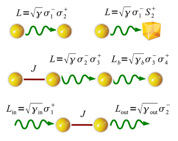
Figure 1: Summary of the toy-networks analyzed analytically in sections II and III.

Incoherent transfer I: $\bullet\stackrel{{\scriptstyle\gamma}}{{\rightsquigarrow}}\bullet$.

Before turning to analyze the possible implementations and consequences of such an effect, let us summarize the Lindblad operators for incoherent Förster transfer among two sites, $L=\sqrt{\gamma}\sigma_{1}^{-}\sigma_{2}^{+}$. This process can be pictorially visualized by the following diagram, $\bullet\stackrel{{\scriptstyle\gamma}}{{\rightsquigarrow}}\bullet$ (see also Fig. 1). The quantum master equation is given simply by $\dot{\rho}=\mathcal{L}_{L}\left(\rho\right)$. We denote by $\mathfrak{n}$ the population operator satisfying $\mathfrak{n}|\eta\rangle=\eta|\eta\rangle$ with $\eta=0,1$, and by $n$ its possibly time-dependent expectation value for excitations, i.e. $n=\langle\mathfrak{n}\rangle:=\mathrm{tr}\left(\mathfrak{n}\rho\right)$. Since the effect of the Lindbladian is to transfer a particle from site $1$ to site $2$, the total number operator is a conserved quantity. We therefore obtain a differential equation for the population in the following way: first note that $\dot{n}_{i}=\mathrm{tr}\left(\mathfrak{n}_{i}\dot{\rho}\right)=\mathrm{tr}\left[\mathfrak{n}_{i}\mathcal{L}_{L}\left(\rho\right)\right].$ Given that $n_{1}+n_{2}=n_{\mathrm{tot}}$ is constant in time, it suffices to analyze the population of site 1, $\dot{n}_{1}=-\gamma n_{1}+\gamma\langle\mathfrak{n}_{1}\mathfrak{n}_{2}\rangle$. Now note that in the single-particle sector, $\mathfrak{n}_{\mathrm{tot}}=1$, $\langle\mathfrak{n}_{1}\mathfrak{n}_{2}\rangle=0$ (to see this use $\mathfrak{n}_{\mathrm{tot}}^{2}=\mathfrak{n}_{\mathrm{tot}}+2\mathfrak{n}_{1}\mathfrak{n}_{2}$), leading to a transport equation $\dot{n}_{1}=-\gamma n_{1}$ that can be readily solved for the population at sites 1, $n_{1}\left(t\right)=e^{-\gamma t}n_{1}\left(0\right)$ and 2, $n_{2}\left(t\right)=n_{2}\left(0\right)+\left(1-e^{-\gamma t}\right)n_{1}\left(0\right)$. The jump operator achieves precisely what we expected: the population in site one decreases exponentially at a rate $\gamma$ and the population of site 2 increases accordingly. The same result could have been obtained by solving the (16 dimensional) differential equation for the full density matrix. Starting at time zero with $\rho\left(0\right)=\{\rho_{i,j}\}$ the time-evolved density matrix $\rho\left(t\right)$ is

$$\left(\begin{array}[]{cccc}\rho_{1,1}&e^{-\gamma t/2}\rho_{1,2}&\rho_{1,3}&\rho_{1,4}\\ e^{-\gamma t/2}\rho_{2,1}&e^{-\gamma t}\rho_{2,2}&e^{-\gamma t/2}\rho_{2,3}&e^{-\gamma t/2}\rho_{2,4}\\ \rho_{3,1}&e^{-\gamma t/2}\rho_{3,2}&\left(1-e^{-\gamma t}\right)\rho_{2,2}+\rho_{3,3}&\rho_{3,4}\\ \rho_{4,1}&e^{-\gamma t/2}\rho_{4,2}&\rho_{4,3}&\rho_{4,4}\end{array}\right).$$

It is interesting to note that for some entangled initial states the asymptotic density matrix $\rho\left(t\rightarrow\infty\right)$ is still entangled. The process $\mathcal{L}_{L}$ cannot, however, create entanglement.

Incoherent transfer II: $\bullet\rightsquigarrow\square$.

To model the congestion in the reaction center, let us now substitute the second qubit with a larger $2s+1$ dimensional space.

For this case, we can model a particle conserving transfer process with a jump operator given by $L=\sqrt{\gamma}\sigma_{1}^{-}S_{2}^{+}$ where $S_{2}^{+}$ is a raising operator of the irreducible spin $s$ representation of $SU\left(2\right)$. The population at site 2 is $\mathfrak{N}_{2}=S_{2}^{z}+s\leavevmode{\rm 1\mkern-4.8muI}$. Once again, since the total particle number $\mathfrak{n}_{\mathrm{tot}}=\mathfrak{n}_{1}+\mathfrak{N}_{2}$ is conserved in a given particle sector, one has $\mathfrak{n}_{\mathrm{tot}}\left(t\right)=n_{\mathrm{tot}}$. We then obtain the following differential equation for population at site 1: $\dot{n}_{1}=-\gamma\langle\mathfrak{n}_{1}S_{2}^{-}S_{2}^{+}\rangle$. By noting that $S_{2}^{-}S_{2}^{+}=(\mathfrak{N}_{2}+1)(2s-\mathfrak{N}_{2})$, and employing $\mathfrak{N}_{2}=n_{\mathrm{tot}}-\mathfrak{n}_{1}$, $\mathfrak{N}_{2}^{2}=n_{\mathrm{tot}}^{2}-2n_{\mathrm{tot}}-1+2\mathfrak{n}_{1}$, and $\mathfrak{n}_{1}^{2}=\mathfrak{n}_{1}$, we obtain an explicit differential equation for $n_{1}$:

$$\dot{n}_{1} = -\gamma n_{\mathrm{tot}}\left[(2s+1)-n_{\mathrm{tot}}\right]\,n_{1}$$

$$n_{1}+N_{2} = n_{\mathrm{tot}}.$$

Excitation transfer now occurs at an effective rate which depends on the total population: $\gamma_{\mathrm{eff}}=\gamma n_{\mathrm{tot}}\left[(2s+1)-n_{\mathrm{tot}}\right]$. Note that $0\leq n_{\mathrm{tot}}\leq 2s+1$ and, correctly, $\gamma_{\mathrm{eff}}\left(n_{\mathrm{tot}}=0\right)=\gamma_{\mathrm{eff}}\left(n_{\mathrm{tot}}=2s+1\right)=0$, i.e. no transfer takes place when the network is either completely empty or completely full. The maximum transfer rate is attained when the condition $n_{\mathrm{tot}}=\left(2s+1\right)/2$ is satisfied. The lesson we get from this slightly modified example, is that transferring excitations to an object with more than just two levels, is likely to result in a population dependent transfer rate.

Interplay between coherent hopping and transfer: $\bullet\stackrel{{\scriptstyle J}}{{\leftrightarrow}}\bullet\stackrel{{\scriptstyle\gamma}}{{\rightsquigarrow}}\bullet\stackrel{{\scriptstyle\gamma_{b}}}{{\rightsquigarrow}}\bullet$.

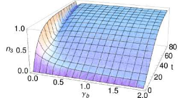
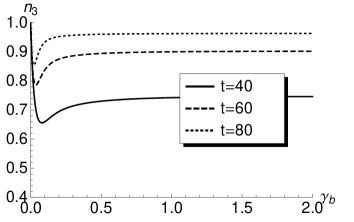
Figure 2: Top panel: The population $n_{3}$ for the case described in section II , as a function of time and $\gamma_{b}$. In this model, the initial state has two excitations at sites 1 and 2: $|1,1,0,0\rangle$. The parameters for the model are $J=1,\,\gamma=0.1$. Bottom: panel: Slices of the same plot at different times are shown. The non-monotonic behavior of the population as a function of the rate $\gamma_{b}$ is evident at small values of it.

We will further illustrate the concept above by considering a variation on the theme. We consider a coherent-hopping Hamiltonian on four sites of the form $H=\left(J/2\right)\left(\sigma_{1}^{-}\sigma_{2}^{+}+\mathrm{h.c.}\right)$ that acts on the first two sites. The excitations are transferred irreversibly from site 2 to site 3 via a quantum jump operator $L=\sqrt{\gamma}\sigma_{2}^{-}\sigma_{3}^{+}$ and subsequently from site 3 to site 4 with $L_{b}=\sqrt{\gamma_{b}}\sigma_{3}^{-}\sigma_{4}^{+}$. $J$ is the coherent coupling strength. In the following, we explore the interplay between the two incoherent transfer rates $\gamma$ and $\gamma_{b}$. Let us focus on the population at site 3, $n_{3}\left(t\right)$. The effect of $\gamma_{b}$ is that of removing excitation population from site 3. However when $\gamma_{b}$ becomes large, excitations are rapidly transferred to site 4 inhibiting the effect of $L_{b}$ ($\mathcal{L}_{b}\left(\rho\right)\rightarrow 0$). This results in a non-trivial non-monotonic effect as a function of $\gamma_{b}$. This feature can be visible only if we have at least two particles in the network. Let us then consider the following initial (pure) state with excitations localized at sites 1 and 2: $|1,1,0,0\rangle$. As shown in Figure 3, in this case, the time-evolution of the populations takes the following form:

$$n_{1}\left(t\right) = C_{1}e^{-\gamma t}+C_{2}e^{-\gamma t/2}+C_{3}\left(t\right)e^{-t\gamma_{b}}$$

$$+C_{4}e^{-t\left(\gamma+\omega\right)/2}+C_{5}e^{-t\left(\gamma-\omega\right)/2}$$

$$n_{2}\left(t\right) = C^{\prime}_{1}e^{-\gamma t}+C^{\prime}_{2}e^{-\gamma t/2}+C^{\prime}_{3}\left(t\right)e^{-t\gamma_{b}}$$

$$+C^{\prime}_{4}e^{-t\left(\gamma+\omega\right)/2}+C^{\prime}_{5}e^{-t\left(\gamma-\omega\right)/2}$$

$$n_{3}\left(t\right) = 1+B_{1}\left(t\right)e^{-t\gamma_{b}}+B_{2}e^{-t\gamma}+B_{3}e^{-t\gamma/2}$$

$$+B_{4}e^{-t\left(\gamma+\omega\right)/2}$$

$$n_{4}\left(t\right) = \frac{\gamma\left(1-e^{-t\gamma_{b}}\right)-\gamma_{b}\left(1-e^{-t\gamma}\right)}{\gamma-\gamma_{b}},$$

where $C_{i},\,C^{\prime}_{i},\,B_{i}$ are only functions of $J,\,\gamma,\,\gamma_{b}$, and $C_{3},\,C^{\prime}_{3},\,B_{1}$ are functions of time as well. Finally $\omega=\sqrt{\gamma^{2}-4J^{2}}$, resulting in an imaginary eigenvalue of the Liouvillian for $2\left|J\right|>\gamma$. This in turn shows up in an oscillating behavior of the populations as a function of time. In Figure 2, the behavior of population 3 as a function of time and $\gamma_{b}$ is plotted for the given values of $J$ and $\gamma$. For large values of $t$, one can observe a non-monotonic behavior as a function of $\gamma_{b}$ emphasized in the bottom panel of Figure 2. This behavior can be qualitatively understood as follows. Consider the behavior of $n_{3}$ as a function of $\gamma_{b}$ for a large fixed time $\tilde{t}$. Since the effect of $\gamma_{b}$ is that of taking away particles from site 3, $n_{3}$ first decreases when $\gamma_{b}$ is increased from zero at fixed $\tilde{t}$. Anyway, if $\gamma_{b}$ is further increased, excitations are taken away at a faster rate and transferred to site 4. This means that at the fixed time $\tilde{t}$ site 4 tends to get full for large $\gamma_{b}$, thus inhibiting the effect of $L_{b}$. Population $n_{3}$ then increases with $\gamma_{b}$. When $\gamma_{b}$ is further increased, site 4 becomes effectively full and $L_{b}$ is turned off, the population becomes then independent of $\gamma_{b}$ and $n_{3}$ saturates.

For the sake of completeness we also consider the solution with one excitation localized at site 1, i.e. $|1,0,0,0\rangle$ at time $t=0$. In this case the time-dependence of the populations is,

$$n_{1}\left(t\right) = \frac{e^{-t\gamma/2}}{\omega^{3}}\left[-2J^{2}\omega+\left(\gamma^{2}-2J^{2}\right)\omega\cosh\left(\frac{t\omega}{2}\right)\right.$$

$$\left.+\gamma\omega^{2}\sinh\left(\frac{t\omega}{2}\right)\right]$$

$$n_{2}\left(t\right) = \frac{2J^{2}e^{-t\gamma/2}}{\omega^{2}}\left[\cosh\left(\frac{t\omega}{2}\right)-1\right]$$

$$n_{3}\left(t\right) = A_{1}e^{-t\gamma_{b}}+A_{2}e^{-t\gamma}+A_{3}e^{-t\left(\gamma+\omega\right)/2}+A_{4}e^{-t\left(\gamma-\omega\right)/2}$$

$$n_{4}\left(t\right) = 1-\sum_{i=1}^{3}n_{i}\left(t\right)$$

where $A_{i}$ are time independent functions of the parameters. One can see in Fig. 3 that the non-monotonic behavior of $n_{3}$ as a function of $\gamma_{b}$ is for this initial condition absent. As expected, since in the network there are no-excitations enough to fill the reaction centre, the “congestion effect” is now absent.

Figure 3: $n_{3}$, as a function of time and $\gamma_{b}$. Initial state has one excitation at sites 1: $|1,0,0,0\rangle$. Parameters are $J=1,\,\gamma=0.05$.

III The staircase effect

In this section, we explore the situation where excitons are fed into a quantum network at a given constant rate $\gamma_{\mathrm{in}}$ and are extracted at a rate $\gamma_{\mathrm{out}}$.

This model can be justified by the fact that some photosynthetic complexes such as purple bacteria and green-sulfur bacteria Ganapathy et al. (2009) live in low-light conditions. The electron-transfer event that occurs in the reaction center is a process that takes place in the order of picoseconds. We therefore take the common practice of modeling the reaction center as an incoherent trap Mohseni et al. (2008).

Injection-extraction: $\stackrel{{\scriptstyle\gamma_{\mathrm{in}}}}{{\rightsquigarrow}}\bullet\stackrel{{\scriptstyle J}}{{\leftrightarrow}}\bullet\stackrel{{\scriptstyle\gamma_{\mathrm{out}}}}{{\rightsquigarrow}}$.

Here, we consider the simplest model for the injection and extraction of an exciton. The model corresponds to two sites coupled coherently via the hopping Hamiltonian, $H=\left(J/2\right)\left(\sigma_{1}^{-}\sigma_{2}^{+}+\sigma_{1}^{+}\sigma_{2}^{-}\right)$. Besides the coherent evolution term, an incoherent injection of excitons is given by a jump operator $L_{\mathrm{in}}=\sqrt{\gamma_{\mathrm{in}}}\sigma_{1}^{+}$ which injects particles at a rate $\gamma_{\mathrm{in}}$ and a corresponding incoherent extraction term $L_{\mathrm{out}}=\sqrt{\gamma_{\mathrm{out}}}\sigma_{2}^{-}$.

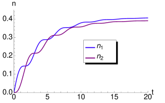
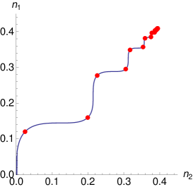
Figure 4: $J=2,$ $\gamma_{\mathrm{in}}=0.2$ (injection), and $\gamma_{\mathrm{out}}=0.3$ (dissipation). Bottom: parametric plot with same parameters. The red dots correspond to times given by $T_{n}=\left(1/2+n\right)T_{0}$, $T_{0}=2\pi/\omega,$ ($n=0,1,\ldots$) and the correct frequency is $\omega=\sqrt{4J^{2}-\left(\gamma_{\mathrm{in}}-\gamma_{\mathrm{out}}\right)^{2}}$. As explained in the text using general arguments, $T_{0}=O\left(J^{-1}\right)$.

The corresponding $16\times 16$ Lindblad superoperator matrix can be diagonalized. A complex eigenvalue with a non-zero imaginary part gives rise to oscillating behavior in the populations when $\left|\gamma_{\mathrm{in}}-\gamma_{\mathrm{out}}\right|<2\left|J\right|$.

Let us first concentrate on the asymptotic state of the evolution, $\rho\left(t\rightarrow\infty\right)$. Solving $\mathcal{L}_{\mathrm{tot}}\left(\rho\right)=0,$ one realizes that the asymptotic state is unique and independent of the initial state. Although this feature is expected in natural physical systems and follows, for instance, from the detailed balance hypothesis, it is not necessarily satisfied in our simple toy models (see e.g. Sec. II).

In the standard basis, $\left\{|1,1\rangle,\,|1,0\rangle,\,|0,1\rangle,\,|0,0\rangle\right\}$, the explicit expression of the asymptotic state is

$$\rho\left(\infty\right)=\frac{1}{\left(\gamma_{\mathrm{in}}+\gamma_{\mathrm{out}}\right)\left(J^{2}+\gamma_{\mathrm{in}}\gamma_{\mathrm{out}}\right)}\times\\ \left(\begin{array}[]{cccc}\frac{J^{2}\gamma_{\mathrm{in}}^{2}}{\left(\gamma_{\mathrm{in}}+\gamma_{\mathrm{out}}\right)}&0&0&0\\ 0&\frac{\gamma_{\mathrm{in}}\gamma_{\mathrm{out}}\left(J^{2}+\left(\gamma_{\mathrm{in}}+\gamma_{\mathrm{out}}\right)^{2}\right)}{\left(\gamma_{\mathrm{in}}+\gamma_{\mathrm{out}}\right)}&iJ\gamma_{\mathrm{in}}\gamma_{\mathrm{out}}&0\\ 0&-iJ\gamma_{\mathrm{in}}\gamma_{\mathrm{out}}&\frac{J^{2}\gamma_{\mathrm{in}}\gamma_{\mathrm{out}}}{\left(\gamma_{\mathrm{in}}+\gamma_{\mathrm{out}}\right)}&0\\ 0&0&0&\frac{J^{2}\gamma_{\mathrm{out}}^{2}}{\left(\gamma_{\mathrm{in}}+\gamma_{\mathrm{out}}\right)}\end{array}\right).$$

The only non-vanishing correlations are $\langle\sigma_{1}^{z}\sigma_{2}^{z}\rangle$, $\langle\sigma_{1}^{z}\rangle$ and $\langle\sigma_{2}^{z}\rangle$. Thus this state is separable but has non vanishing classical correlations: $\langle\sigma_{1}^{z}\sigma_{2}^{z}\rangle-\langle\sigma_{1}^{z}\rangle\langle\sigma_{2}^{z}\rangle\neq 0$. Equivalently, the asymptotic state is a classical mixture of states with definite populations.

Having $\rho\left(\infty\right)$ we can compute the asymptotic populations:

$$n_{1}\left(\infty\right) = \frac{\gamma_{\mathrm{in}}\left(J^{2}+\gamma_{\mathrm{in}}\gamma_{\mathrm{out}}+\gamma_{\mathrm{out}}^{2}\right)}{\left(\gamma_{\mathrm{in}}+\gamma_{\mathrm{out}}\right)\left(J^{2}+\gamma_{\mathrm{in}}\gamma_{\mathrm{out}}\right)}$$ (1)

$$n_{2}\left(\infty\right) = \frac{\gamma_{\mathrm{in}}J^{2}}{\left(\gamma_{\mathrm{in}}+\gamma_{\mathrm{out}}\right)\left(J^{2}+\gamma_{\mathrm{in}}\gamma_{\mathrm{out}}\right)}.$$ (2)

A few simple facts can be directly seen from equations (1), (2). First, for small $\gamma_{\mathrm{in}}$ populations deviate by $O\left(\gamma_{\mathrm{in}}\right)$ from zero; vice versa for $\gamma_{\mathrm{out}}$ small populations deviate by $O\left(\gamma_{\mathrm{out}}\right)$ from one. Instead, when $J$ is small excitations get loaded at site 1 but take a long time to reach site 2 so that $n_{1}=1-O\left(J^{2}\right)$, $n_{2}=O\left(J^{2}\right)$. Finally, for very large $J$ both populations tend to $n_{1}\simeq n_{2}=\gamma_{\mathrm{in}}/\left(\gamma_{\mathrm{in}}+\gamma_{\mathrm{out}}\right)+O\left(J^{-2}\right)$.

Let us now turn to the dynamics and consider first the most interesting case namely when the initial state is the empty state $|0,0\rangle$. A typical result is shown in figure 4. An interesting feature clearly emerges: when population $n_{\mathrm{1}}$ increases, $n_{2}$ stays almost constant and vice-versa. Such a feature is particularly evident in the parametric plot. In the lower panel of figure 4 we also stressed another peculiarity of this process: the time needed to increase a given population when the other is constant (i.e. the horizontal and vertical steps between two red dots in Fig. 4), is always the same. We call $T_{0}$ this new, emerging, time-scale. The description of the entire process then is the following. First particles are injected at site 1 and population at site 2 stays zero until a time $T_{0}/2$. Next, for $T_{0}/2<t<3/2T_{0}$ the situation is reverted and population 2 increases while population 1 remains constant. The process continues in this fashion until an asymptotic state is reached. Given the shape of the curve in Fig. 4 we refer to this situation as “staircase effect”. The emerging time-scale can be given a physical interpretation considering the limit when both injection and extraction rates are very small. In this case the only time-scale of the system is given by the time needed for the excitations to hop from site 1 to site 2. This time is given by $T_{0}\approx\Delta E^{-1}=O\left(J^{-1}\right)$. In general, if we substitute the two sites with an open chain of length $L$, using the same argument we expect (at least for small $\gamma_{\mathrm{in}}$, $\gamma_{\mathrm{out}}$) that $T_{0}$ will be the time needed for the excitations to travel from one side of the chain to the other, i.e. $T_{0}\approx L/v$ where $v$ is the velocity of quasiparticles. Of course this picture can be correct only as long as a quasi-particle description applies (cf. Sec. V.3).

Let us now consider the injection-extraction dynamics with an initial state $|1,0\rangle$, i.e. at time zero the injection site is occupied. A typical (in the oscillating regime) scenario is shown in Fig. 5. Starting with an initial state $|0,1\rangle$, the situation is almost identical with $n_{\mathrm{1}}$ and $n_{2}$ interchanged. In fact, one can show that for initial states with one definite excitation, populations at any time satisfy the following duality relation

$$n_{1}\left(\gamma_{\mathrm{in}},\gamma_{\mathrm{out}}\right)=1-n_{2}\left(\gamma_{\mathrm{out}},\gamma_{\mathrm{in}}\right).$$

As previously explained the asymptotic populations do not depend on the initial populations and are still given by equations (1) and (2). The parametric plot in the lower panel of Fig. 5 shows that with this initial condition the staircase effect is not present.

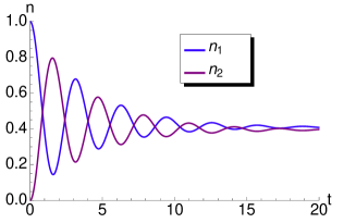
Figure 5: $|1,0\rangle$. Parameters are $J=2$ $\gamma_{\mathrm{in}}=0.2$ (pump) and $\gamma_{\mathrm{out}}=0.3$ (dissipation). Below: parametric plot, same parameters.

Three-site injection-extraction: $\stackrel{{\scriptstyle\gamma_{\mathrm{in}}}}{{\rightsquigarrow}}\bullet\stackrel{{\scriptstyle J}}{{\leftrightarrow}}\bullet\stackrel{{\scriptstyle J}}{{\leftrightarrow}}\bullet\stackrel{{\scriptstyle\gamma_{\mathrm{out}}}}{{\rightsquigarrow}}$.

A slight generalization of the above idea is given by a three site chain with injection on the first site and extraction on the third. For simplicity we consider a uniform chain with equal couplings $J_{12}=J_{23}=J$. In this case the asymptotic populations are given by

$$n_{1}\left(\infty\right) = \frac{\gamma_{\mathrm{in}}\left(J^{2}+\gamma_{\mathrm{in}}\gamma_{\mathrm{out}}+\gamma_{\mathrm{out}}^{2}\right)}{\left(\gamma_{\mathrm{in}}+\gamma_{\mathrm{out}}\right)\left(J^{2}+\gamma_{\mathrm{in}}\gamma_{\mathrm{out}}\right)}$$

$$n_{2}\left(\infty\right) = \frac{\gamma_{\mathrm{in}}\left(J^{2}+\gamma_{\mathrm{out}}^{2}\right)}{\left(\gamma_{\mathrm{in}}+\gamma_{\mathrm{out}}\right)\left(J^{2}+\gamma_{\mathrm{in}}\gamma_{\mathrm{out}}\right)}$$

$$n_{3}\left(\infty\right) = \frac{\gamma_{\mathrm{in}}J^{2}}{\left(\gamma_{\mathrm{in}}+\gamma_{\mathrm{out}}\right)\left(J^{2}+\gamma_{\mathrm{in}}\gamma_{\mathrm{out}}\right)}.$$

Note that populations $n_{1}$ and $n_{3}$ are the same as $n_{1}$, $n_{2}$ in the previous, two-site case. Starting from the totally empty state, the asymptotic state is reached in a similar manner as in the two-site case. In particular, the parametric plot of the injection and extraction sites $\left(n_{1}\left(t\right),n_{3}\left(t\right)\right)$ displays a staircase shape exactly as in the two site case. As we will show in Sec. V.3, this feature survives even in a longer chain, and is to some extent resistant to small static diagonal disorder and dephasing.

IV Asymptotic unitarity

Another effect we want to study is the possibility that a coherent dynamics (or sub-dynamics) may emerge out of a dissipative or partly incoherent dynamics. To make things more clear let us immediately discuss the simplest example showing this feature.

Hopping and transfer: $\bullet\stackrel{{\scriptstyle J}}{{\leftrightarrow}}\bullet\stackrel{{\scriptstyle\gamma}}{{\rightsquigarrow}}\bullet$.

The model consists of three sites (qubits). On the first two sites acts a coherent hopping of the form $H=\left(J/2\right)\left(\sigma_{1}^{-}\sigma_{2}^{+}+\sigma_{1}^{+}\sigma_{2}^{-}\right)$. On top of that, particles are transferred irreversibly from site 2 to site 3 via a jump operator given by $L=\sqrt{\gamma}\sigma_{2}^{-}\sigma_{3}^{+}$. It is clear that, if a particle sits at site 3 the incoherent part of the dynamics is not effective, that is $\mathcal{L}_{L}\left[\rho_{12}\otimes|1\rangle\langle 1|\right]=0$. If we start with an initial state $|1,1,0\rangle$ with sites 1 and 2 occupied and site 3 empty, for effect of the dynamics, site 3 will get populated at a rate $\gamma$, and on the first two sites there will remain one particle coherently hopping back and forth. By this we mean that for a sufficiently large time the evolved state will be similar to a coherent evolution: $\rho\left(t\right)=e^{t\mathcal{L}_{\mathrm{tot}}}\left[\rho\right]\simeq e^{-itH}\tilde{\rho}e^{itH}=:\tilde{\rho}\left(t\right)$. For what concerns the state $\tilde{\rho}$ we only know that it will contain one particle; it can be obtained by evolving back unitarily $\rho\left(t\right)$, i.e.

$$\tilde{\rho}=\lim_{t\rightarrow\infty}e^{itH}\rho\left(t\right)e^{-itH}.$$

Indeed, if the dynamics becomes unitary, the above limit is well defined. Notice that $\tilde{\rho}$ is nothing but the stationary solution of the original master equation in the interaction picture associated with $H$. The same reasoning can be done for the subsystem consisting on sites 1 and 2, i.e. we can define $\tilde{\rho}_{1,2}$ by evolving back unitarily $\rho_{1,2}\left(t\right)$. Since $H$ does not act on site 3 we have $\tilde{\rho}_{1,2}=\mathrm{tr}_{3}\tilde{\rho}$. An explicit computation confirms that $\tilde{\rho}=\tilde{\rho}_{1,2}\otimes|1\rangle\langle 1|$, i.e. in the equivalent, unitary dynamics, one particle sits at site 3. The explicit form of $\tilde{\rho}_{1,2}$ in the standard basis is

$$\tilde{\rho}_{1,2}=\frac{1}{2\left(J^{2}+\gamma^{2}\right)}\left(\begin{array}[]{cccc}0&0&0&0\\ 0&J^{2}+2\gamma^{2}&-iJ\gamma&0\\ 0&iJ\gamma&J^{2}&0\\ 0&0&0&0\end{array}\right).$$

This state is a quantum superposition of one-particle states with $n_{1}=1/2+\gamma^{2}/2\left(J^{2}+\gamma^{2}\right)$ and $n_{2}=1/2-\gamma^{2}/2\left(J^{2}+\gamma^{2}\right)$.

What are the possible indicators of asymptotic unitarity? Since the purity is constant under unitary evolution, one possibility is to look at the purity of the total system or of some part of it. The time-derivative of such a quantity will then be close to zero, for approximate unitary evolution. Since for Lindbladian evolution the purity derivative is $\partial_{t}\mathrm{tr}\left(\rho^{2}\right)=2\mathrm{tr}\left[\rho\left(t\right)\mathcal{L}_{\mathrm{tot}}\left(\rho\right)\right]$, this definition has the advantage of being numerically stable. In our toy model we have

$$\mathrm{tr}\left\{\left[\rho_{1,2}\left(t\right)\right]^{2}\right\}=\mathrm{tr}\left[\rho^{2}\right]=1-\frac{J^{2}}{2\left(J^{2}+\gamma^{2}\right)}+\\ \frac{-2e^{-\gamma t}\left(J^{2}+\gamma^{2}+\gamma^{2}\cos\left(Jt\right)\right)+e^{-2\gamma t}\left(3J^{2}+4\gamma^{2}\right)}{2\left(J^{2}+\gamma^{2}\right)}.$$

Unfortunately the purity tends to a constant whenever the solution tends to a constant, as happens, for instance, along the natural process reaching the asymptotic state. In other words, the smallness of the purity derivative is a sufficient but not necessary condition for asymptotic unitarity.

Another possibility is to measure some distance between the actual state and the one obtained with unitary evolution: $\left\|\rho\left(t\right)-\tilde{\rho}\left(t\right)\right\|$. Once again, we might as well restrict to a particular subsystem. Using the operator norm the result for our toy-model is particularly simple and illuminating

$$\left\|\rho\left(t\right)-\tilde{\rho}\left(t\right)\right\|=\left\|\rho_{1,2}\left(t\right)-\tilde{\rho}_{1,2}\left(t\right)\right\|=e^{-\gamma t}.$$

This confirms our initial intuition: the dynamics becomes unitary at a rate $\gamma$. This approach has a very clear meaning but has the disadvantage of being computationally demanding as it requires the computation of a matrix norm and the evaluation of $\tilde{\rho}\left(t\right)$. A simpler alternative is the following.

Consider the spectral representation of the Hamiltonian $H=\sum_{n}E_{n}|n\rangle\langle n|$. If the total evolution becomes similar to a unitary evolution, the matrix elements of the density matrix in the eigenbasis $|n\rangle$ evolve in time like phases:

$$\langle n|\rho\left(t\right)|m\rangle\simeq\langle n|\tilde{\rho}\left(t\right)|m\rangle=e^{-it\left(E_{n}-E_{m}\right)}\langle n|\tilde{\rho}|m\rangle.$$

In our model the eigenbasis of the two-site Hamiltonian is $\{|0,0\rangle,\,|1,1\rangle,\,|\psi^{\pm}\rangle=\left(|1,0\rangle\pm|0,1\rangle\right)/\sqrt{2}\}$. For instance, one can show that

$$\langle\psi^{-}|\rho_{1,2}\left(t\right)|\psi^{+}\rangle=\frac{\gamma}{iJ+\gamma}\left(e^{-t\gamma}-\cos\left(Jt\right)-i\sin\left(Jt\right)\right).$$

Pictorially the parametric plot of the real and imaginary part of this matrix element folds on a circle (of radius $\gamma/\sqrt{J^{2}+\gamma^{2}}$) after a time $\gamma^{-1}$ (see Fig. 6).

This method to mark the appearance of asymptotic unitarity, as well as the study of the distance $\left\|\rho\left(t\right)-\tilde{\rho}\left(t\right)\right\|$, has a major advantage with respect to those based on $\dot{\rho}\left(t\right)$. Namely it allows to discriminate between approximate unitary evolution and the usual reach of an asymptotic state for which $\dot{\rho}=0$.

We would like to end this section by stressing the (almost obvious) relation of asymptotic unitarity with the quantum-information concept of noiseless or decoherence-free subspace/system Zanardi and Rasetti (1997). The quantum networks considered in this paper are of hybrid type, namely some of the inter-site couplings are coherent i.e., hopping, and other are incoherent i.e., irreversible transfer described by $L.$ On the other hand, the dynamics restricted to the range of the projection $P:=\openone_{12}\otimes|1\rangle\langle 1|$ is unitary because, as noticed in the above, $\mathcal{L}_{L}(P\rho P)=0.$ This means that the range of $P$ is indeed a decoherence-free subspace. Now the dynamics is such that, for appropriate initial conditions $\lim_{t\to\infty}n_{3}(t)=1$ or equivalently $\lim_{t\to\infty}\|P\rho(t)P-\rho(t)\|=0$ . This means that the asymptotic state belongs to the range of $P,$ which in turn implies the unitary nature of the long-time dynamics.

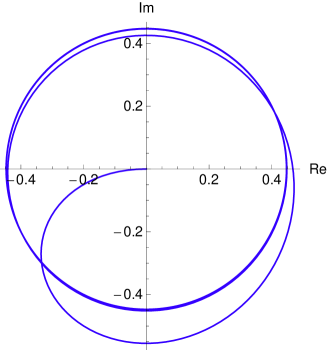
Figure 6: $\langle\psi^{-}|\rho_{1,2}\left(t\right)|\psi^{+}\rangle$ for the model considered in the text. Parameters are $J=2,\,\gamma=1$.

V Applications to LH1-RC complexes

In this section we want to check if and how the effects studied so far can survive in more realistic networks. Specifically, we will consider models which can be relevant for the description of energy transfer in photosynthetic systems.

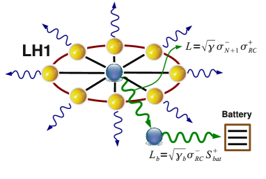
Figure 7: $N$ particles on the ring interact via dimerized nearest neighbor hopping constants $t_{i,i+1}=t\left(1+\delta\left(-1\right)^{i}\right)$. Each of these particle can hop to the central site ($N+1$th) with hopping constant $J$. The central site transfers excitations incoherently to the reaction center via $L=\sqrt{\gamma}\sigma_{N+1}^{-}\sigma_{RC}^{+}$. The reaction center itself is connected to a $(2s+1)-$ dimensional “battery” via $L_{b}=\sqrt{\gamma_{b}}\sigma_{RC}^{-}S_{\mathrm{bat}}^{+}$. The effect of external degrees of freedom is schematized by incoherent dissipation and dephasing processes (thin, blue, wavy lines). In actual LH1 complexes the sites on the ring are bacteriochlorophylls, and $N=32$.

V.1 Congestion effect

Our motivation for the study of the “congestion effect” originated from a careful analysis of the structure of the reaction center in LH1-RC complexes. In most photosynthetic bacteria, photons are captured by light-harvesting antennae where a particle-hole exciton is created and carried to the reaction center (RC) where eventually a redox reaction takes place Blankenship (2002). In the LH1-RC complexes present in purple bacteria the light harvesting complex and the RC form a compact core unit. Typical transfer times of excitations to the RC are of the order of hundreds of picoseconds. A cartoon picture of the LH1-RC complex is shown in figure 7. Yellow spheres represents the bacteriochlorophylls forming LH1. In the purple bacterium Rodobacter sphaeroides, there are 32 bacteriochlorophylls (BChl) displaced on a ring surrounding the reaction center. In figure 7 we display a possible structure for the RC. Instead of treating the RC as a simple two-level system, as typically done in the literature, we replace the RC with a structure containing two qubits and a $d$-level system which we call a “battery”. In purple bacteria this structure has to be imagined sitting at the center of the ring. The first of these qubits (the $N+1$th) interacts via coherent dipole-dipole hopping with the BChls of the ring. Excitations are then transferred at a rate $\gamma$ to what we call reaction center. In turn, the RC itself is connected to larger $d$-level system ($d=3$ in our simulations) via irreversible transfer at a rate $\gamma_{b}$. It is the interplay between the two timescales $\gamma^{-1}$ and $\gamma_{b}^{-1}$, and their relation to the transfer efficiency, that we want to analyze here.

The master equation for the whole system is of Lindblad type: $\dot{\rho}=-i\left[H,\rho\right]+\mathcal{L}_{\mathrm{tot}}\left(\rho\right)$. For what we said so far, the incoherent part is given by $\mathcal{L}_{\mathrm{tot}}=\mathcal{L}_{L}+\mathcal{L}_{L_{b}}+\mathcal{L}_{\mathrm{noise}}$ with $L=\sqrt{\gamma}\sigma_{N+1}^{-}\sigma_{RC}^{+}$ and $L_{b}=\sqrt{\gamma_{b}}\sigma_{RC}^{-}S_{bat}^{+}$. Dissipation and dephasing effects are taken into account via incoherent terms acting on the sites of the ring $\mathcal{L}_{\mathrm{noise}}=\sum_{j=1}^{N}\mathcal{L}_{L_{j,\mathrm{diss}}}+\mathcal{L}_{L_{j,\mathrm{deph}}}$ with $L_{j,\mathrm{diss}}=\sqrt{\gamma_{\mathrm{diss}}}\sigma_{j}^{-}$ and $L_{j,\mathrm{deph}}=\sqrt{\gamma_{\mathrm{deph}}}\mathfrak{n}_{j}$.

Regarding the Hamiltonian of the ring degrees of freedom, we referred to the detailed structure of couplings given in Hu et al. (1997); Hu and Schulten (1998). The most salient feature emerging from the data of Hu and Schulten (1998) is that the couplings present a dimerized structure: strong coupling $t_{+}=t\left(1+\delta\right)$ alternate with weak ones $t_{-}=t\left(1-\delta\right)$. Indeed, instead of using all the couplings $t_{i,j}$ reported Hu and Schulten (1998), almost the same band structure can be obtained using only a nearest neighbor description with a dimerization of $\delta=0.12$. Some groups have suggested the possibility that dimerization might favor the transfer efficiency Yang et al. (2010). Our choice of resorting to a dimerized nearest neighbor hopping structure has the additional advantage of making the system scalable to different sizes $N$. Hence our choice for the Hamiltonian is

$$H=\sum_{j=1}^{N}t_{j}\left(\sigma_{j}^{-}\sigma_{j+1}^{+}+\sigma_{j}^{+}\sigma_{j+1}^{-}\right)+J\left(\sigma_{j}^{-}\sigma_{N+1}^{+}+\sigma_{j}^{+}\sigma_{N+1}^{-}\right).$$

This represents $N$ particles on a ring hopping between neighboring sites with constants $t_{j}=t\left(1+\delta\left(-1\right)^{j}\right)$ and to a central site $N+1$ with hopping constant $J$. We will also add static random diagonal noise ($H\rightarrow H+\sum_{j}\epsilon_{j}\mathfrak{n}_{j}$) to inhibit the possible appearance of decoherence-free subspaces which can limit the efficiency of transfer Caruso et al. (2009).

The results of our simulations are shown in Fig. 8. We initialize the system by starting with a pure Dicke state for the ring while keeping all other sites empty. This means the initial state is $|\psi_{0}\rangle=\left(\begin{array}[]{c}N\\ n\end{array}\right)^{-1/2}\left(\sigma_{\mathrm{tot}}^{+}\right)^{n}|0\rangle$ where $\sigma_{\mathrm{tot}}^{+}=\sum_{j=1}^{N}\sigma_{j}^{+}$ refers only to the ring sites and $|0\rangle$ is the empty state for the whole system. The choice of an initial Dicke state is natural for a series of reasons. First it allows to treat initial states with general definite particle number $n\leq N$. Second, Dicke states are symmetric under permutation, thus carrying no net momentum. If the photon’s wavelength is larger than the size of the LH1 complex, the excitations created must be a completely delocalized $k=0$ object. In any case, since only the $k=0$ component of the ring couples to the central $N+1$th site, transfer in the antisymmetric channel $k=\pi$, being a higher order process, is highly suppressed and gives much lower transfer efficiency Olaya-Castro et al. (2008).

We first performed simulations on a “clean” system, i.e. with no dissipation or dephasing present. In Fig. 8 we plotted the population of the reaction center (normally called efficiency $\eta$ in the literature) as a function of time for different values of $\gamma_{b}$. Looking at the upper panels of Fig. 8, the situation is completely analogous to the congestion effect observed in our simple toy model (see Figures 2, 3). As long as we start with a number of excitations which can be accommodated in the battery, they will all flow to the battery for $\gamma_{b}\neq 0$ (left panel). When we start with 3 particles in the ring we see again the appearance of a non-monotonic behavior between $\gamma_{b}$ and $\gamma$ which shows up as a valley at large times and $\gamma_{b}\lesssim\gamma$ ($\gamma_{b}$ smaller than, but of the order of $\gamma$). When we add additional decoherence in the form of dissipation and dephasing the situation is only quantitatively changed. The valley due to the “congestion effect”, although less pronounced, is still visible in the bottom right panel of Fig. 8.

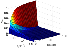
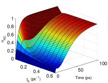
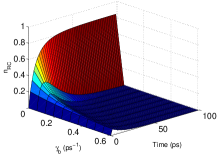
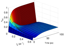
Figure 8: “congestion effect” in light-harvesting complexes. Upper panels: clean system, no dissipation and dephasing. The ring has $N=4$ sites, hopping constants are $t=J=1\,(meV)$ and dimerization is $\delta=0.12$. Diagonal static noise of the form $\epsilon_{n}=t\cos\left(en\right)$ is added. The RC transfer rate is set to $\gamma=0.3\,ps^{-1}$. Lower panels: same parameters plus dissipation and dephasing $\gamma_{\mathrm{diss}}=\gamma_{\mathrm{deph}}=0.03\,ps^{-1}$. Left panels: the initial state is a two-particle Dicke state for the ring, other sites are empty. Right panels: the initial state is a three-particle Dicke state for the ring, other sites are empty.

V.2 Asymptotic unitarity

To study asymptotic unitarity the “battery” is an unnecessary complication. Therefore, we will use the same model of Fig. 7 without the battery site and the corresponding jump operator. This leads to a network of $N+2$ qubits where the $N+1$th site is connected to the RC via irreversible transfer at a rate $\gamma$. As done previously, we will use an $n$-particle Dicke state as the initial state. Let us first consider the case where the only incoherent term is the one transferring particles from the central site to the RC. In this case the dynamics becomes exactly unitary when the RC is full. Simulations on a network with $N+2=6$ qubits are shown in Fig. 9. We also show the effect of dissipation and dephasing, though one order of magnitude smaller than the RC transfer. For short times the evolution is the same as for the clean (i.e. no dissipation and dephasing) case, however for time of order $\gamma_{\mathrm{diss}}^{-1}$ dissipation sets in and the parametric plot for a generic matrix element $\langle n|\rho\left(t\right)|m\rangle$, spirals down to zero (Fig. 9 bottom right plot).

The conclusion of this section is as simple as it is intriguing, in view of potential applications to biological systems. If the time-scale $\gamma_{\mathrm{diss}}^{-1}$ is large enough, there may exist a time window $T_{\mathrm{relax}}<t<\gamma_{\mathrm{diss}}^{-1}$ in which quantum effects are not only visible but the dynamics is effectively unitary! In our models $T_{\mathrm{relax}}$ is the time needed for the RC to get filled, and is of the order of $T_{\mathrm{relax}}\sim\gamma^{-1}$. Even more important is the fact that the incoherent transfer to the RC must shut down when the RC is full. Considering the LH1-RC complex, the separation of time-scales does indeed occur. For instance in Olaya-Castro et al. (2008); Fassioli et al. (2010) the dissipation is four orders of magnitude smaller than the RC charge-separation rate. Whether the RC shuts down when it is occupied, although plausible, is much harder to assess.

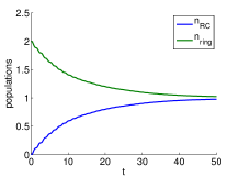
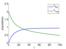
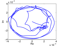
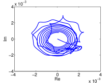
Figure 9: $N+2=6$ sites. On the upper panels we plot the populations of the ring and of the RC as a function of time (arbitrary units). Bottom panels: parametric plot of the real and imaginary parts of a matrix element $\langle\psi_{m}|\langle 1|\rho\left(t\right)|\psi_{n}\rangle|1\rangle$ for certain $m,\,n$. $|\psi_{n}\rangle$ are the Hamiltonian eigenstates. Left panels: the Hamiltonian has $t=J=1$, $\delta=0.12,$ diagonal static noise $\epsilon_{p}=t\cos\left(ep\right),$ and no dissipation or dephasing. Excitations are transferred to the RC at a rate $\gamma=0.2$. Right panels: same parameters, but on the particles of the ring acts dissipation and dephasing with $\gamma_{\mathrm{deph}}=\gamma_{\mathrm{diss}}=0.01$.

V.3 Staircase effect

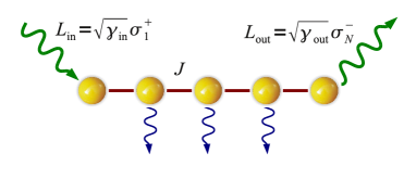
Figure 10: $N$ sites interact via a nearest-neighbor hopping Hamiltonian. Particles are injected, and respectively expelled incoherently at rates $\gamma_{\mathrm{in}}$, $\gamma_{\mathrm{out}}$ on the first and last sites . On top of this basic structure we can add static diagonal disorder and dissipation as well as dephasing (symbolized by blue wavy arrows) $\mathcal{L}_{\mathrm{noise}}=\sum_{j=2}^{N-1}\mathcal{L}_{L_{j,\mathrm{diss}}}+\mathcal{L}_{L_{j,\mathrm{deph}}}$.

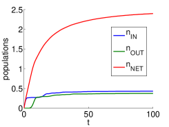
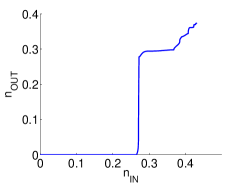
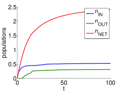
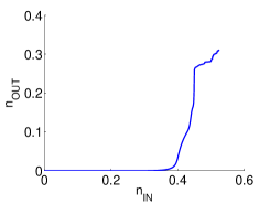
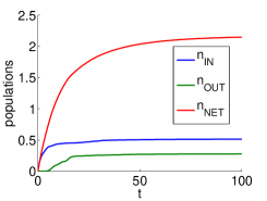
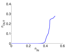
Figure 11: $J=1$ and $\gamma_{\mathrm{in}}=0.2$, $\gamma_{\mathrm{out}}=0.3$. First row panels: neither dissipation nor dephasing, and no static noise. Second row panels: addition of diagonal static noise $\epsilon_{n}=J\cos\left(en\right)$. Third row panels: static noise plus dissipation and dephasing $\gamma_{\mathrm{diss}}=\gamma_{\mathrm{deph}}=10^{-2}$.

Here we want to show that the staircase effect, studied in Sec. III, survives in more elaborate networks. We will study this effect in the model depicted in Fig. 10. The model consists of an open chain of $N$ sites hopping coherently between nearest neighbors, i.e. the Hamiltonian is

$$H=\sum_{j=1}^{N-1}J\left(\sigma_{j}^{-}\sigma_{j+1}^{+}+\sigma_{j}^{+}\sigma_{j+1}^{-}\right).$$

Particles are injected into the first site of the chain via a jump operator $L_{\mathrm{in}}=\sqrt{\gamma_{\mathrm{in}}}\sigma_{1}^{+}$ and taken away at the last site via $L_{\mathrm{out}}=\sqrt{\gamma_{\mathrm{out}}}\sigma_{N}^{-}$. On top of this basic framework we add different layers of complexity. First we can add some static random diagonal noise, i.e. we add site dependent energies to the coherent part $H\rightarrow H+\sum_{j}\epsilon_{j}\mathfrak{n}_{j}$. Second we can also include dissipation and dephasing acting on the inner sites of the chain by adding the following superoperator: $\mathcal{L}_{\mathrm{noise}}=\sum_{j=2}^{N-1}\mathcal{L}_{L_{j,\mathrm{diss}}}+\mathcal{L}_{L_{j,\mathrm{deph}}}$ ($L_{j,\mathrm{diss}}=\sqrt{\gamma_{\mathrm{diss}}}\sigma_{j}^{-}$ and $L_{j,\mathrm{deph}}=\sqrt{\gamma_{\mathrm{deph}}}\mathfrak{n}_{j}$ as defined previously).

The picture that we have is the following. Through the coherent part of the evolution, excitations travel in the chain in packets of quasiparticles at velocities $v_{k}=O\left(J\right)$ ($k$ is a quasi-momentum label). This introduces a lag timescale $T_{0}\approx L/v\sim O\left(L/J\right)$, which is the time needed for an excitation to travel from one side of the chain to the other. From Fig. 11 (all panels) we see that, when the population at the injection site increases, the population at the expulsion site stays constant during this time-lag $T_{0}$ and vice versa. Considering the central and lower panel of Fig. 11 we can appreciate how robust the effect is with respect to various type of “perturbations”. The addition of static random noise has the effect of localizing states and shuffling the single-particle dispersion $\epsilon_{k}$. Both of these effects destroy the picture of wavepackets traveling at constant velocity, in that both the traveling times and the dispersion of the wave-packets increase. Instead the addition of dissipation (and dephasing) to the network, mostly has the effect of relaxing the system at a faster rate. As long as the system has not relaxed the effect remains visible. Comparatively, the presence of static coherent noise hinders the stair-case effect more to dissipation and dephasing.

VI Conclusions

Inspired by the models which are recently being used to describe energy transfer in photosynthetic pigments, we have identified and discussed a few effects arising in quantum networks with coherent (Hamiltonian) as well as incoherent (Lindblad) coupling between the nodes. For the reader’s sake we summarize here below these basic effects

1. Congestion effect. The incoherent transfer of excitations is inversely proportional to the population in the reaction center. This is due to the hard-core nature of the excitations that effectively reduces the amplitude of the jump operator as the reaction center fills.

2. Asymptotic unitarity. Coherent, unitary evolution may emerge out of a dissipative, incoherent dynamics. This happens if states which annihilate the incoherent part of the dynamics can be reached during the time evolution. For this effect to be observable one needs a separation of time-scales, $T_{\mathrm{relax}}\ll T_{\mathrm{diss}}$. Such separation of time-scales does take place in some photosynthetic systems e.g. in the LH1-RC complexes present in purple bacteria.

3. Staircase effect. This effect refers to a situation in which particles are injected incoherently, travel coherently along a given chain, and then are expelled (or digested) at a certain rate at the other end of the chain. The effect of the coherent part is to introduce a time-scale $T_{0}=O\left(L/v\right)=O\left(L/J\right)$, ($L$ is the system size, $v$ the velocity of excitations and $J$ is the energy scale of the coherent network). $T_{0}$ is roughly the time needed for the excitations to travel from one side of the chain to the other. The peculiar feature emerging from the dynamic evolution, is that when the population at the injection site increases, the population at the expulsion site stays constant during this time-lag $T_{0}$ and vice versa. This effect results in a step-like behavior in the parametric plot of the injection/extraction populations.

The effects we analyzed in this paper can be traced back to very simple mechanisms displayed even by networks composed by only few qubits. We provided analytical solutions for these toy models and showed numerical evidence that these effects survive in more elaborated network such as those modeling energy transfer in purple bacteria. Clearly, further investigations are in order to establish the relevance of the elementary calculations presented in this paper to the newborn field of quantum biology.

The authors are sincerely in debt with Alán Aspuru-Guzik who played a vital role in the early stage of this project. We also thank N. Toby Jacobson for a careful reading of the manuscript. P.Z. acknowledges support from NSF grants PHY-803304, DMR-0804914 and L.C.V. acknowledges support from European project COQUIT under FET-Open grant number 2333747.

References

- Blankenship (2002) R. Blankenship, Molecular mechanisms of photosynthesis (Blackwell Science, Oxford; Malden, MA, 2002).
- van Grondelle and Novoderezhkin (2006) R. van Grondelle and V. Novoderezhkin, Phys. Chem. Chem. Phys. 8, 793 (2006).
- Milder et al. (2010) M. Milder, a. R. v. G. B. Bruggemann, et al., Photosynth. Res. 104, 257 (2010).
- Adolphs and Renger (2006) J. Adolphs and T. Renger, Biophys. J. 91, 2778 (2006).
- Renger (2009) T. Renger, Photosynth. Res. 102, 471 (2009).
- Ritz et al. (2001) T. Ritz, S. Park, and K. Schulten, J. Phys. Chem. B 105, 8259 (2001).
- Brixner et al. (2005) T. Brixner et al., Nature 434, 625 (2005).
- Engel et al. (2007) G. Engel, T. Calhoun, E. Read, et al., Nature 446, 782 (2007).
- Collini et al. (2010) E. Collini, C. Wong, K. Wilk, et al., Nature 463, 644 (2010).
- Panitchayangkoon et al. (2010) G. Panitchayangkoon, D. Hayes, K. Fransted, et al., PNAS 107, 12766 (2010).
- Schlau-Cohen et al. (2010) G. Schlau-Cohen, T. Calhoun, N. Ginsberg, et al., PNAS 107, 13276 (2010).
- Womick et al. (2010) J. M. Womick, S. A. Miller, and A. M. Moran, J. Chem. Phys. 133, 024507 (2010).
- Gaab and Bardeen (2004) K. Gaab and J. Bardeen, J. Chem. Phys. 121, 7813 (2004).
- Mohseni et al. (2008) M. Mohseni, P. Rebentrost, S. Lloyd, and A. Aspuru-Guzik, J. Chem. Phys. 129, 174106 (2008).
- Rebentrost et al. (2009a) P. Rebentrost, M. Mohseni, I. Kassal, S. Lloyd, and A. Aspuru-Guzik, New J. Phys. 11, 033003 (2009a).
- Rebentrost et al. (2009b) P. Rebentrost, M. Mohseni, and A. Aspuru-Guzik, J. Phys. Chem B 113, 9942 (2009b).
- Plenio and Huelga (2008) M. B. Plenio and S. Huelga, New J. Phys 10, 113019 (2008).
- Caruso et al. (2009) F. Caruso, A. Chin, A. Datta, et al., J. Chem. Phys. 131, 105106 (2009).
- Cao and Silbey (2009) J. S. Cao and R. Silbey, J. Chem. Phys. A 113, 13825 (2009).
- Wu et al. (2010) J. Wu, F. Liu, Y. Shen, et al., New J. Phys. 12, 105012 (2010).
- Mulken and Schmid (2010) O. Mulken and T. Schmid, Phys. Rev. D 82, 042104 (2010).
- Cao (1997) J. Cao, J. Chem. Phys. 107, 3204 (1997).
- Renger and Marcus (2002) T. Renger and R. Marcus, J. Chem. Phys. 116, 9997 (2002).
- Olaya-Castro et al. (2008) A. Olaya-Castro, C. Lee, F. Olsen, et al., Phys. Rev. B 78, 085115 (2008).
- Ishizaki and Fleming (2009) A. Ishizaki and G. Fleming, J. Chem. Phys. 130, 234111 (2009).
- Lloyd and Mohseni (2010) S. Lloyd and M. Mohseni, New J. Phys. 12, 075020 (2010).
- Zhu et al. (2010) J. Zhu, S. Kais, P. Rebentrost, and A. Aspuru-Guzik (2010), accepted by J. Phys. Chem. B.
- Nazir (2009) A. Nazir, Phys. Rev. Lett 103, 146404 (2009).
- Nalbach et al. (2010) P. Nalbach, J. Eckel, and M. Thorwart, New J. Phys. 12, 065043 (2010).
- Fassioli and Olaya-Castro (2010) F. Fassioli and A. Olaya-Castro, New J. Phys. 12, 085006 (2010).
- Fassioli et al. (2010) F. Fassioli, A. Nazir, and A. Olaya-Castro, J. Phys. Chem. Lett. 14, 2139 (2010).
- Wöhri et al. (2010) A. Wöhri et al., Science 328, 630 (2010).
- Ganapathy et al. (2009) S. Ganapathy, G. Oostergetel, P. Wawrzyniak, M. Reus, A. Chew, F. Buda, E. Boekema, D. Bryant, A. Holzwarth, and H. de Groot, PNAS 106, 8525 (2009).
- Zanardi and Rasetti (1997) P. Zanardi and M. Rasetti, Phys. Rev. Lett. 79, 3306 (1997).
- Hu et al. (1997) X. Hu et al., J. Phys. Chem. B 101, 3854 (1997).
- Hu and Schulten (1998) X. Hu and K. Schulten, Biophys. J. 75, 683 (1998).
- Yang et al. (2010) S. Yang, D. Xu, Z. Song, and C. Sun, J. Chem. Phys. 132, 234501 (2010).