Bogoliubov Excitations of Disordered Bose-Einstein Condensates

Abstract

We describe repulsively interacting Bose-Einstein condensates in spatially correlated disorder potentials of arbitrary dimension. The first effect of disorder is to deform the mean-field condensate. Secondly, the quantum excitation spectrum and condensate population are affected. By a saddle-point expansion of the many-body Hamiltonian around the deformed mean-field ground state, we derive the fundamental quadratic Hamiltonian of quantum fluctuations. Importantly, a basis is used such that excitations are orthogonal to the deformed condensate. Via Bogoliubov-Nambu perturbation theory, we compute the effective excitation dispersion, including mean free paths and localization lengths. Corrections to the speed of sound and average density of states are calculated, due to correlated disorder in arbitrary dimensions, extending to the case of weak lattice potentials.

I Introduction

The intriguing interplay of Bose statistics, interaction, and disorder is one of the most prominent problems in condensed matter physics, known as the dirty boson problem Giamarchi and Schulz (1987); *Giamarchi1988; Fisher et al. (1989). Experimentally, it was first studied with superfluid Helium in aerosol glasses (Vycor) Crooker et al. (1983); *Chan1988; *Wong1990. Over the past years, several groups have loaded ultracold atoms into optical potentials and studied Bose-Einstein condensates (BECs) in the presence of disorder under very clean laboratory conditions Clément et al. (2005); Schulte et al. (2005); Lye et al. (2005); Chen et al. (2008); White et al. (2009); Dries et al. (2010).

In this paper, we study the situation where Bose statistics and interaction are the dominant effects, and the disorder weakly perturbs the homogeneous situation. In this regime, the presence of a well-populated condensate makes Bogoliubov’s theory Bogoliubov (1947) the most economic description, because it describes quantum fluctuations around the best mean-field approximation of the condensate.

What happens to a homogeneous condensate if a weak external potential is switched on? How are the quantum fluctuations affected? These questions constitute the inhomogeneous Bogoliubov problem, a problem of notorious difficulty, due to the broken translational symmetry Nozières and Pines (1999). Bogoliubov theories for disordered BEC have been formulated by Lee and Gunn Lee and Gunn (1990), Huang and Meng Huang and Meng (1992) and Giorgini, Pitaevskii and Stringari Giorgini et al. (1994), complemented by Kobayashi and Tsubota (2002); Astrakharchik et al. (2002); Bilas and Pavloff (2006); Lugan et al. (2007); Falco et al. (2007); Fontanesi et al. (2009); Hu et al. (2009), among others. Yet, none of the existing theories covers spatially correlated disorder and all dimensionalities, which come into focus after recent experimental advances Lewenstein et al. (2007); Bloch et al. (2008); Sanchez-Palencia and Lewenstein (2010); Modugno (2010); Robert-de-Saint-Vincent et al. (2010).

Moreover, some approaches appear questionable from a conceptual point of view. Indeed, the primary effect of an external potential is to deform the condensate itself. This is most obvious for cold-atom BECs in traps, where the condensate forms in a non-uniform spatial mode that results from the competition between interaction, kinetic, and potential energy. Therefore, it is awkward, if not outright inappropriate, to construct a Bogoliubov theory in terms of fluctuations that are still defined as deviations from the uniform condensate of the homogeneous case Huang and Meng (1992); Kobayashi and Tsubota (2002); Astrakharchik et al. (2002); Falco et al. (2007); Hu et al. (2009). Instead, Bogoliubov’s ansatz warrants to first determine the deformed condensate mode on the mean-field level. Accordingly, we discuss the number-conserving deformation of the condensate caused by a weak external potential in Section II.1.

The deformed condensate is the vacuum of Bogoliubov fluctuations, to whose description we turn in a second step. Great care must be taken to ensure that the excitations occur in modes that remain orthogonal to the inhomogeneous ground state—even in a disordered situation where the ground state depends on each realization of the random potential. We have found it helpful to tackle this formidable problem by a variational saddle-point expansion, a powerful method central to the solution of many problems in statistical and quantum mechanics Kleinert (2009); Giamarchi and Le Doussal (1996). Such an expansion yields all relevant terms in a systematic manner, without the need for deciding ad hoc which terms are to be kept or discarded. Section II.2 contains a full account of our formulation, leading to the fundamental inhomogeneous Bogoliubov Hamiltonian that is quadratic in the fluctuations.

We emphasize that our approach describes both effects, the deformation of the ground state and the scattering of excitations, on the same footing and to the same order in the external potential. Moreover, our approach involves quantized fluctuations that always remain orthogonal to the inhomogeneous Bogoliubov vacuum. A fully analytical description is presented up to second order in disorder strength.

The excitation spectrum of any system provides precious information about its (thermo-)dynamic properties. For instance, the homogeneous interacting Bose gas has a gapless excitation spectrum. This is consistent with the fact that the low-energy excitations are the Goldstone modes Goldstone et al. (1962) associated with the spontaneous $U(1)$ symmetry breaking in the BEC phase. These low-energy excitations are collective in character, with many interacting particles oscillating back and forth as in a sound wave. And really, the dispersion relation at low energy is linear, its slope being the sound velocity. The sound velocity is intimately linked to numerous important quantities like specific heat and compressibility, and moreover, by a classical argument due to Landau, equal to the critical velocity of superfluidity Dalfovo et al. (1999); Pethick and Smith (2002); Pitaevskii and Stringari (2003).

Since an external potential couples to the particle density and does not interfere with the $U(1)$ symmetry, it is not expected to induce an excitation gap. However, inhomogeneity should certainly affect the speed of sound, which is a nonlinear function of the particle density. Thus, it is of particular interest to predict the speed-of-sound correction in disordered Bose gases. But curiously, the state of affairs for this key quantity is far from satisfactory. The simplest Bogoliubov theories cannot predict a change in excitation dispersion at all Huang and Meng (1992); Kobayashi and Tsubota (2002); Astrakharchik et al. (2002). More elaborate calculations by Giorgini et al. Giorgini et al. (1994) predict a certain positive correction for uncorrelated disorder in three dimensions, a result which has been exactly reproduced by Lopatin and Vinokur Lopatin and Vinokur (2002) and Falco et al. Falco et al. (2007). This is contradicted by Yukalov and Graham Yukalov and Graham (2007); Yukalov et al. (2007) who report a decrease of the sound velocity in three dimensions, even in the case of uncorrelated disorder. A negative correction is also found, in all dimensions, for spatially correlated disorder with a correlation length much longer than the condensate healing length Gaul et al. (2009).

Clearly, there is a need for a unified theory that describes the dispersion relation of Bogoliubov excitations in presence of disorder with spatial correlation. In section III, we provide such a theory, at least perturbatively for weak external potentials, by applying standard diagrammatic Green function techniques to the inhomogeneous Bogoliubov Hamiltonian derived in Sec. II.2. We compute the ensemble-averaged disorder correction to the single-excitation spectrum in general, including the elastic scattering rate, and corrections to sound velocity and density of states.

In Section IV, these general results are discussed in greater detail, with particular emphasis on the case of correlated disorder. Numerous analytical results are found in certain limiting regions of the parameter space, which is spanned by condensate healing length, excitation wave length, and disorder correlation length. Specific results pertaining to optical speckle potentials are collected in Appendix A. In passing, we recover the localization properties of Bogoliubov excitations in one dimension as described earlier by Bilas and Pavloff Bilas and Pavloff (2006) and Lugan et al. Lugan et al. (2007). We briefly connect to the case of weak lattice potentials and confirm predictions by Taylor and Zaremba Taylor and Zaremba (2003) and Liang et al. Liang et al. (2008) within our formalism. We also reconfirm the positive correction of the speed of sound by uncorrelated disorder in three dimensions Giorgini et al. (1994); Lopatin and Vinokur (2002); Falco et al. (2007). It turns out, though, that this result is hardly generic, because in lower dimensions and for correlated disorder in general, one always finds a negative correction. We confirm our analytical predictions in one dimension by numerical simulations on the mean field level, as well as by exact numerical diagonalization of the Bogoliubov-de Gennes equations.

Finally, Section V concludes and closes the paper on some open questions.

II The inhomogeneous Bogoliubov Hamiltonian

A weakly interacting Bose gas is described by the (grand canonical) Hamiltonian Dalfovo et al. (1999); Pethick and Smith (2002); Pitaevskii and Stringari (2003)

$$\hat{E}=\int {\rm d}^{d}r\,\hat{\Psi}^{\dagger}\left[\frac{-\hbar^{2}}{2m}\nabla^{2}+V({\boldsymbol{r}})-\mu+\frac{g}{2}\hat{\Psi}^{\dagger}\hat{\Psi}\right]\hat{\Psi},$$ (1)

in terms of particle annihilation and creation operators $\hat{\Psi}=\hat{\Psi}({\boldsymbol{r}})$ and $\hat{\Psi}^{\dagger}=\hat{\Psi}^{\dagger}({\boldsymbol{r}})$, respectively, which obey the canonical commutator relations

$$\begin{split}\bigl{[}\hat{\Psi}({\boldsymbol{r}}),\hat{\Psi}({\boldsymbol{r}}^{\prime})\bigr{]}&=\bigl{[}\hat{\Psi}^{\dagger}({\boldsymbol{r}}),\hat{\Psi}^{\dagger}({\boldsymbol{r}}^{\prime})\bigr{]}=0,\\ \bigl{[}\hat{\Psi}({\boldsymbol{r}}),\hat{\Psi}^{\dagger}({\boldsymbol{r}}^{\prime})\bigr{]}&=\delta({\boldsymbol{r}}-{\boldsymbol{r}}^{\prime}).\end{split}$$ (2)

Atom-atom interaction is taken into account in the form of s-wave scattering. The s-wave scattering length $a_{\rm s}$ determines the interaction parameter, $g={4\pi\hbar^{2}}a_{\rm s}/{m}$ in three dimensions, with similar relations in quasi-two and quasi-one dimensional geometries. We will treat the case of repulsive interaction with a constant interaction parameter $g>0$. This interaction potential is a good approximation in the regime of low energy and dilute gases, where the gas parameter $(na_{\rm s}^{3})^{1/2}$ is small, i.e., the average particle distance $n^{-1/3}$ is much larger than the scattering length $a_{\rm s}$. For dilute ultracold gases (unlike superfluid helium), this parameter is typically very small $(na_{\rm s}^{3})^{1/2}\approx 0.01$ Pitaevskii and Stringari (1998).

We will work in the canonical ensemble with a fixed total number of particles $N=\int{\rm d}^{d}r\bigl{\langle}\hat{\Psi}^{\dagger}({\boldsymbol{r}})\hat{\Psi}({\boldsymbol{r}})\bigr{\rangle}$. The chemical potential $\mu$ serves as the Lagrange parameter that has to be adjusted accordingly, as function of external control parameters. One of these external control fields is the inhomogeneous external potential $V({\boldsymbol{r}})$. In the laboratory, this typically comprises a global trapping potential as well as, say, optical lattices and/or disorder potentials. In the following, we will concentrate on the situation where the global trapping potential is very smooth, ideally a very large box, and $V({\boldsymbol{r}})$ then describes the local spatial fluctuations around the homogeneous background.

Below a critical temperature, the Bose gas forms a BEC Einstein , where a macroscopically large fraction of particles populates the ground state of the single-particle density matrix. In the absence of interaction, this is just the ground state of the potential $V({\boldsymbol{r}})$, but also in a dilute interacting Bose gas a well defined condensate mode appears, as proven rigorously in the homogeneous case and three dimensions Lieb and Seiringer (2002); Erdős et al. (2007). Within a mean-field description (or equivalently, Hartree-Fock theory) the condensate spontaneously breaks the U(1) gauge invariance of the Hamiltonian (1) by settling on a global phase. In lower dimensions and within confining potentials, quasi-condensates Mora and Castin (2003) exist, whose phase coherence is not of truly infinite range, but can extend over large enough distances such that the condensate shows the tell-tale signatures of a phase-coherent matter wave.

Bogoliubov’s theory Bogoliubov (1947) takes advantage of the macroscopically occupied ground state of the BEC and splits the field operator into a mean-field condensate and quantized fluctuations:

$$\hat{\Psi}({\boldsymbol{r}})=\Phi({\boldsymbol{r}})+\delta\hat{\Psi}({\boldsymbol{r}}).$$ (3)

The small parameter of this expansion is again the gas parameter $(na_{\rm s}^{3})^{1/2}$ Lee et al. (1957), and for dilute condensed atomic gases, Bogoliubov theory proves to be a very adequate description.

Following this approach, we will first describe how the external potential $V({\boldsymbol{r}})$ affects the condensate mode, strictly within mean field. In a second step, we determine the relevant Hamiltonian of the quantum fluctuations around this modified ground state. We emphasize from the outset that a consistent Bogoliubov theory requires to calculate both steps to the same order in $V({\boldsymbol{r}})$; otherwise one runs the risk of describing only half of the relevant physics. Instead of deciding ad hoc which terms should be kept and which not, we resort to a well-controlled saddle-point expansion of the many-body Hamiltonian around the mean-field ground state.

II.1 Deformed mean-field ground state

The mean-field approach, known as Gross-Pitaevskii (GP) theory Gross (1963); Pitaevskii and Stringari (2003), neglects the quantum fluctuations and replaces the field operators by a complex field $\Psi=\Psi({\boldsymbol{r}})$, such that the many-body Hamiltonian (1) reduces to the GP energy functional:

$$E=\int{\rm d}^{d}r\biggl{\{}\frac{\hbar^{2}}{2m}|\boldsymbol{\nabla}\Psi|^{2}+\big{[}V({\boldsymbol{r}})-\mu\big{]}|\Psi|^{2}+\frac{g}{2}|\Psi|^{4}\biggr{\}}.$$ (4)

We wish to determine its ground state as function of the external potential $V({\boldsymbol{r}})$. By definition, the ground state $\Psi_{0}({\boldsymbol{r}})=\Phi({\boldsymbol{r}})$ minimizes the energy functional (4). It obeys the stationarity condition $\left.\delta E/\delta\Psi^{*}\right|_{0}=0$, also known as the stationary GP equation

$$-\frac{\hbar^{2}}{2m}{\nabla^{2}\Phi({\boldsymbol{r}})}+(g|\Phi({\boldsymbol{r}})|^{2}-\mu){\Phi({\boldsymbol{r}})}=-V({\boldsymbol{r}}){\Phi({\boldsymbol{r}})}.$$ (5)

For a stationary potential $V({\boldsymbol{r}})$, the condensate’s kinetic energy is always minimized by choosing a fixed global phase, thereby ruling out superfluid flow or vortices, and without loss of generality we may take $\Phi({\boldsymbol{r}})\in\mathbb{R}$ in the following.

In the homogeneous case $V({\boldsymbol{r}})=0$, the repulsive interaction spreads the density over the entire available volume, and $n=|\Phi|^{2}=\mu/g$. In the inhomogeneous case, however, the condensate wave function depends via Eq. (5) nonlinearly on $V({\boldsymbol{r}})$. Numerically, the condensate $\Psi({\boldsymbol{r}})$ can be computed very efficiently, for any given potential $V({\boldsymbol{r}})$, by propagating the GP equation in imaginary time Dalfovo and Stringari (1996).

What analytical tools are available? If the external potential and the condensate wave function vary only very smoothly, the first term in Eq. (5), the kinetic energy or quantum pressure, is negligible. In this so-called Thomas-Fermi (TF) regime, the density profile is then determined by the balance of interaction and external potential,

$$n_{\rm TF}({\boldsymbol{r}})=\frac{1}{g}[\mu-V({\boldsymbol{r}})]$$ (6)

where $V({\boldsymbol{r}})<\mu$ and $n_{\rm TF}({\boldsymbol{r}})=0$ else. But in a potential that varies on short length scales, the kinetic energy term becomes relevant, and the TF result no longer suffices.

If the external potential is small, $V\ll gn\approx\mu$, the imprint on the condensate amplitude can be computed perturbatively Sanchez-Palencia (2006). We expand

$$\Phi({\boldsymbol{r}})=\Phi^{(0)}+\Phi^{(1)}({\boldsymbol{r}})+\Phi^{(2)}({\boldsymbol{r}})+\ldots,$$ (7)

around the homogeneous solution $\Phi^{(0)}=\sqrt{n}$ in powers of the small parameter $V/\mu\ll 1$. In order to maintain a fixed average particle density $L^{-d}\int{\rm d}^{d}r|\Phi({\boldsymbol{r}})|^{2}=n$, also the chemical potential is adjusted at each order,

$$\mu =\mu^{(0)}+\mu^{(1)}+\mu^{(2)}+\ldots, \mu^{(0)} =gn.$$ (8)

We insert these expansions into Eq. (5) and collect orders up to $V^{2}/\mu^{2}$. Because the kinetic energy $\epsilon^{0}_{k}=\hbar^{2}k^{2}/2m$ is diagonal in $k$-space, solving for the $\Phi^{(i)}$ and $\mu^{(i)}$ is best done in momentum representation, $\Phi_{\boldsymbol{k}}=\left\langle{\boldsymbol{k}}\right|\Phi\rangle=L^{-d/2}\int{\rm d}^{d}re^{-i{\boldsymbol{k}}\cdot{\boldsymbol{r}}}\Phi({\boldsymbol{r}})$ and $V_{\boldsymbol{k}}=\left\langle{\boldsymbol{k}}+{\boldsymbol{k}}^{\prime}\right|V\left|{\boldsymbol{k}}^{\prime}\right\rangle=L^{-d}\int{\rm d}^{d}re^{-i{\boldsymbol{k}}\cdot{\boldsymbol{r}}}V({\boldsymbol{r}})$.

The first-order imprint of the potential in the condensate amplitude reads

$$\Phi^{(1)}_{\boldsymbol{k}}=-\frac{(1-\delta_{{\boldsymbol{k}}0})V_{\boldsymbol{k}}}{\epsilon^{0}_{k}+2gn}N^{1/2}.$$ (9)

As expected for linear response, the shift is directly proportional to the potential’s matrix element $V_{\boldsymbol{k}}$. The Kronecker delta stems from the first-order shift $\mu^{(1)}=V_{0}$ that compensates the potential average, ensuring $\Phi^{(1)}_{0}=0$ as required by conservation of average particle density.

In the denominator, the comparison between interaction $gn$ and kinetic energy defines a characteristic length scale of the BEC, the healing length $\xi=\hbar/\sqrt{2mgn}$. Factoring out $gn$, one is left with $2+\epsilon^{0}_{k}/gn=2+k^{2}\xi^{2}$ in the denominator. This term becomes constant for long-range potential variations with $k\xi\to 0$, and one recovers the TF imprint (6) for the density $n({\boldsymbol{r}})=|\Phi({\boldsymbol{r}})|^{2}=n+n^{(1)}({\boldsymbol{r}})$, in Fourier components $n^{(1)}_{{\boldsymbol{k}}\text{TF}}=-V_{\boldsymbol{k}}/g$. In the contrary case $k\xi\gg 1$, this denominator suppresses short-scale potential variations. Indeed, the condensate avoids rapid variations, which cost too much kinetic energy, and responds only to a smoothed component of the external potential Sanchez-Palencia (2006).

Figure 1 shows a 1D real-space plot of the condensate density deformed by a rather strong Gaussian impurity potential of width $\sigma=0.8\xi$. For such a small impurity, the full numerical solution differs greatly from the simple TF formula (6). The first-order smoothing result (9) already gives much better agreement. However, we need to push the expansion even further, in order to obtain consistent second-order results later on.

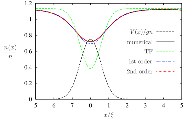
Figure 1: (Color online) Condensate density $n(x)$ deformed by an impurity potential $V(x)=V\exp(-x^{2}/\sigma^{2})$ (dashed black) with $V=0.75gn$ and $\sigma=0.8\xi$. The numerical solution of the GP equation (5) [solid black, under periodic boundary conditions within the shown interval] differs significantly from the TF result (6) [dashed green]. Including first-order (11) and second-order smoothing (13) terms improves the agreement.

Solving for the second order imprint brings about terms of two different types. Viewing the GP equation (5) as a scattering equation for the field $\Phi$ Wellens and Grémaud (2009); Gaul (2010), one finds first a contribution from double scattering by the external potential $V({\boldsymbol{r}})$ with free propagation in between. Secondly, there is a contribution from the interaction of two single-scattered amplitudes $\Phi^{(1)}$. Altogether, including the chemical potential shift, the second-order condensate deformation reads

$$\Phi^{(2)}_{\boldsymbol{k}} =\frac{1}{N^{1/2}}\sum_{\boldsymbol{p}}\Phi^{(1)}_{{\boldsymbol{k}}-{\boldsymbol{p}}}\Phi^{(1)}_{{\boldsymbol{p}}}\frac{(1-\delta_{{\boldsymbol{k}}0})\epsilon^{0}_{p}-gn}{2gn+\epsilon^{0}_{k}}.$$ (10)

For future reference, we also write down the leading-order terms for the Fourier components of the condensate density $n({\boldsymbol{r}})=|\Phi({\boldsymbol{r}})|^{2}$, the inverse field $\check{\Phi}({\boldsymbol{r}})=n/\Phi({\boldsymbol{r}})$, as well as the inverse density $\check{n}({\boldsymbol{r}})=n^{2}/n({\boldsymbol{r}})$. To linear order, one has of course $\check{\Phi}^{(1)}_{\boldsymbol{k}}=-\Phi^{(1)}_{\boldsymbol{k}}$ as well as

$$n^{(1)}_{\boldsymbol{k}}=-\check{n}^{(1)}_{\boldsymbol{k}}=-2n\frac{(1-\delta_{{\boldsymbol{k}}0})V_{\boldsymbol{k}}}{2gn+\epsilon^{0}_{k}},$$ (11)

using the Fourier convention $n_{\boldsymbol{k}}=L^{-d}\int{\rm d}^{d}re^{-i{\boldsymbol{k}}\cdot{\boldsymbol{r}}}n({\boldsymbol{r}})$ for $n$ and $\check{n}$, in the same way as for $V$. Eq. (11) is the linear response of the condensate density to the external potential Giorgini et al. (1994).

To second order, one finds

$$\check{\Phi}^{(2)}_{\boldsymbol{k}} =\frac{1}{N^{1/2}}\sum_{\boldsymbol{p}}\Phi^{(1)}_{{\boldsymbol{k}}-{\boldsymbol{p}}}\Phi^{(1)}_{{\boldsymbol{p}}}\frac{\epsilon^{0}_{k}-(1-\delta_{{\boldsymbol{k}}0})\epsilon^{0}_{p}+3gn}{2gn+\epsilon^{0}_{k}},$$ (12)

$$n^{(2)}_{\boldsymbol{k}} =\frac{1-\delta_{{\boldsymbol{k}}0}}{L^{d}}\sum_{\boldsymbol{p}}\Phi^{(1)}_{{\boldsymbol{k}}-{\boldsymbol{p}}}\Phi^{(1)}_{{\boldsymbol{p}}}\frac{2\epsilon^{0}_{p}+\epsilon^{0}_{k}}{2gn+\epsilon^{0}_{k}},$$ (13)

$$\check{n}^{(2)}_{\boldsymbol{k}} =\frac{1}{L^{d}}\sum_{\boldsymbol{p}}\Phi^{(1)}_{{\boldsymbol{k}}-{\boldsymbol{p}}}\Phi^{(1)}_{{\boldsymbol{p}}}\frac{3\epsilon^{0}_{k}-2(1-\delta_{{\boldsymbol{k}}0})\epsilon^{0}_{p}+8gn}{2gn+\epsilon^{0}_{k}}.$$ (14)

In Figure 1, the results of second-order smoothing are practically indistinguishable from the full solution of the GP equation.

We note at last that even an external potential with zero mean causes a negative shift of the chemical potential,

$$\mu^{(2)}=-\frac{1}{N}\sum_{{\boldsymbol{q}}}\epsilon^{0}_{q}|\Phi^{(1)}_{\boldsymbol{q}}|^{2}=-\sum_{\boldsymbol{q}}\epsilon^{0}_{q}\frac{|V_{\boldsymbol{q}}|^{2}(1-\delta_{{\boldsymbol{q}}0})}{(2gn+\epsilon^{0}_{q})^{2}}.$$ (15)

A negative chemical potential shift must occur non-perturbatively, as can be seen by spatially integrating the GP equation (5) after dividing by $\Phi({\boldsymbol{r}})$: the positivity of the kinetic energy entails that the chemical potential shift, at fixed average particle density, must be negative Lee and Gunn (1990).

This concludes our calculation of the inhomogeneous GP ground state, and we turn to the fluctuations around this condensate.

II.2 Bogoliubov Excitations

Using the Bogoliubov ansatz (3), we expand the Hamiltonian (1) in powers of $\delta\hat{\Psi}$ and $\delta\hat{\Psi}^{\dagger}$. To zeroth order, we find the GP ground-state energy $E_{0}=E[\Phi({\boldsymbol{r}})]$. The linear term vanishes, because $\Phi({\boldsymbol{r}})$ minimizes the energy functional (4). The relevant contribution is then the quadratic part, $\hat{E}=E_{0}+\hat{H}$. Third-order and forth-order terms in the fluctuations are neglected. They describe interaction between the excitations and become only relevant for larger densities or higher temperatures Katz et al. (2002).

For reasons that will become clear in Sec. II.2.5 below, the inhomogeneous Bogoliubov Hamiltonian is best expressed in density-phase variables. From $\hat{\Psi}=\exp\{i\delta\hat{\varphi}\}\sqrt{n+\delta\hat{n}}=\Phi+\delta\hat{n}/2\Phi+i\Phi\delta\hat{\varphi}+\dots$ follows

$$\delta\hat{n}({\boldsymbol{r}}) =\Phi({\boldsymbol{r}})\left\{\delta\hat{\Psi}^{\dagger}({\boldsymbol{r}})+\delta\hat{\Psi}({\boldsymbol{r}})\right\},$$ (16a)

$$\delta\hat{\varphi}({\boldsymbol{r}}) =\frac{i}{2\Phi({\boldsymbol{r}})}\left\{\delta\hat{\Psi}^{\dagger}({\boldsymbol{r}})-\delta\hat{\Psi}({\boldsymbol{r}})\right\},$$ (16b)

up to higher orders in $\delta\hat{\Psi}$. The commutators (2) imply that density and phase (fluctuation) operators are conjugate, $\bigl{[}\delta\hat{n}({\boldsymbol{r}}),\delta\hat{\varphi}({\boldsymbol{r}}^{\prime})\bigr{]}=i\delta({\boldsymbol{r}}-{\boldsymbol{r}}^{\prime})$. By expanding the many-body Hamiltonian to second order in the fluctuations around the mean-field solution, the relevant Hamiltonian for the excitations is found as Gaul and Müller (2008)

$$\hat{H}=\int{\rm d}^{d}r\biggl{\{}\frac{\hbar^{2}}{2m}\biggl{[} \left({\boldsymbol{\nabla}}\frac{\delta\hat{n}}{2\Phi({\boldsymbol{r}})}\right)^{2}+\frac{\left[\nabla^{2}\Phi({\boldsymbol{r}})\right]}{4\Phi^{3}({\boldsymbol{r}})}\delta\hat{n}^{2}$$

$$+\Phi^{2}({\boldsymbol{r}})({\boldsymbol{\nabla}}\delta\hat{\varphi})^{2}\biggr{]}+\frac{g}{2}\,\delta\hat{n}^{2}\biggr{\}}.$$ (17)

With Eq. (17), the problem is reduced to a Hamiltonian that is quadratic in the excitations. To this order, there are no mixed terms of $\delta\hat{n}$ and $\delta\hat{\varphi}$. The perturbing potential $V({\boldsymbol{r}})$ does not appear directly. Instead, it enters nonlinearly via the condensate function $\Phi({\boldsymbol{r}})$, which can be predetermined by solving the GP equation (5) or calculated perturbatively, as explained in the previous Sec. II.1.

Before further discussing the impact of the external potential, we briefly consider the excitations of the homogeneous system.

II.2.1 Homogeneous Bogoliubov Hamiltonian

In the homogeneous case $V({\boldsymbol{r}})=0$, the Bogoliubov Hamiltonian (17) becomes translation invariant and thus diagonal in the momentum representation $\delta\hat{n}_{\boldsymbol{k}}=L^{-d/2}\int{\rm d}^{d}re^{-i{\boldsymbol{k}}\cdot{\boldsymbol{r}}}\delta\hat{n}({\boldsymbol{r}})$ and $\delta\hat{\varphi}_{\boldsymbol{k}}=L^{-d/2}\int{\rm d}^{d}re^{-i{\boldsymbol{k}}\cdot{\boldsymbol{r}}}\delta\hat{\varphi}({\boldsymbol{r}})$:

$$\hat{H}^{(0)} =\sum_{{\boldsymbol{k}}}\left[n\epsilon^{0}_{k}\,{\delta\hat{\varphi}_{{\boldsymbol{k}}}^{\dagger}}{\delta\hat{\varphi}_{\boldsymbol{k}}}+\frac{2gn+\epsilon^{0}_{k}}{4n}\,\delta\hat{n}_{\boldsymbol{k}}^{\dagger}\delta\hat{n}_{\boldsymbol{k}}\right]$$ (18)

with $\epsilon^{0}_{k}=\hbar^{2}k^{2}/2m$. This Hamiltonian looks diagonal, but the Heisenberg equations of motion for $\delta\hat{n}_{\boldsymbol{k}}=\delta\hat{n}_{-{\boldsymbol{k}}}^{\dagger}$ and $\delta\hat{\varphi}_{\boldsymbol{k}}=\delta\hat{\varphi}_{-{\boldsymbol{k}}}^{\dagger}$, which obey

$$[\delta\hat{n}_{\boldsymbol{k}},\delta\hat{\varphi}_{{\boldsymbol{k}}^{\prime}}^{\dagger}]=i\delta_{{\boldsymbol{k}}{\boldsymbol{k}}^{\prime}},$$ (19)

are still coupled. This is resolved by a Bogoliubov transformation Bogoliubov (1947), coupling density and phase fluctuations to quasiparticle creation and annihilation operators $\hat{\gamma}^{\dagger}_{\boldsymbol{k}}$ and $\hat{\gamma}_{\boldsymbol{k}}$:

$$\left(\begin{array}[]{c}\hat{\gamma}_{{\boldsymbol{k}}}\\ \hat{\gamma}^{\dagger}_{-{\boldsymbol{k}}}\end{array}\right)=A_{k}\left(\begin{array}[]{c}i\sqrt{n}\,\delta\hat{\varphi}_{{\boldsymbol{k}}}\\ \delta\hat{n}_{\boldsymbol{k}}/2\sqrt{n}\end{array}\right),\quad A_{k}=\left(\begin{array}[]{cc}a_{k}&a_{k}^{-1}\\ -a_{k}&a_{k}^{-1}\end{array}\right).$$ (20)

A transformation of this kind, with the free parameter $a_{k}$, guarantees that the quasiparticles obey bosonic commutation relations

$$\bigl{[}\hat{\gamma}_{{\boldsymbol{k}}},\hat{\gamma}^{\dagger}_{{\boldsymbol{k}}^{\prime}}\bigr{]} =\delta_{{\boldsymbol{k}}{\boldsymbol{k}}^{\prime}}, \bigl{[}\hat{\gamma}_{{\boldsymbol{k}}},\hat{\gamma}_{{\boldsymbol{k}}^{\prime}}\bigr{]}=\bigl{[}\hat{\gamma}^{\dagger}_{{\boldsymbol{k}}},\hat{\gamma}^{\dagger}_{{\boldsymbol{k}}^{\prime}}\bigr{]} =0.$$ (21)

The Hamiltonian (18) becomes diagonal,

$$\hat{H}^{(0)}=\sum_{{\boldsymbol{k}}}\,\epsilon_{k}\hat{\gamma}^{\dagger}_{{\boldsymbol{k}}}\hat{\gamma}_{{\boldsymbol{k}}},$$ (22)

by choosing

$$a_{k}=\left(\frac{\epsilon_{k}}{\epsilon^{0}_{k}}\right)^{1/2}=\left(\frac{k^{2}\xi^{2}}{2+k^{2}\xi^{2}}\right)^{\frac{1}{4}}.$$ (23)

The excitations are found to have the famous Bogoliubov dispersion relation Bogoliubov (1947)

$$\epsilon_{k}=\sqrt{\epsilon^{0}_{k}(2gn+\epsilon^{0}_{k})}=gn\,k\xi\sqrt{2+k^{2}\xi^{2}},$$ (24)

plotted in Figure 2(a) for reference.

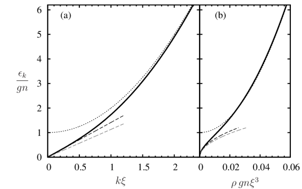
Figure 2: Bogoliubov excitations in the homogeneous condensate. (a) Bogoliubov dispersion relation (24) (solid). (b) Density of states (26) in three dimensions (solid). In both panels, dashed and dotted lines show the low-energy and high-energy asymptotics, respectively. The gray dashed lines foreshadow the disorder corrections provided in Sec. IV.

In the high-energy or large-momentum regime $k\xi\gg 1$, the excitations are essentially free particles with dispersion $\epsilon^{0}_{k}$, shifted by the condensate background energy,

$$\epsilon_{k}\approx\epsilon^{0}_{k}+gn.$$ (25)

In the low-energy regime, the interaction dominates over the bare kinetic energy. A single excitation involves many individual particles, comparable to a classical sound wave. Indeed, the dispersion relation is linear, $\epsilon_{k}=\hbar ck$, with the bare sound velocity $c=\sqrt{gn/m}$. According to a classical argument due to Landau (Pethick and Smith, 2002, chapter 10.1), this linear dispersion at low energies implies superfluidity with critical velocity $v_{c}=\min_{k}(\epsilon_{k}/{\hbar k})=c$.

The transition from sound-wave to single-particle excitations also reflects in the density of states (DOS)

$$\rho(\epsilon) =\frac{S_{d}k_{\epsilon}^{d-1}}{(2\pi)^{d}}\left|\frac{\partial k}{\partial\epsilon}\right|_{k_{\epsilon}}\Theta(\epsilon)$$ (26)

with $S_{d}=2,2\pi,4\pi$ the surface of the $d$-dimensional sphere in $d=1,2,3$, respectively. The $k$-vector at energy $\epsilon$ is given by $k^{2}_{\epsilon}\xi^{2}=[1+(\epsilon/gn)^{2}]^{1/2}-1$. Eq. (26) shows the transition from a sound-wave DOS $\rho_{\rm sw}(\epsilon)\propto\epsilon^{d-1}$ to particle DOS $\rho_{\rm pt}(\epsilon+gn)\propto\epsilon^{\frac{d}{2}-1}$, as illustrated in Figure 2(b) for $d=3$.

II.2.2 Inhomogeneous Bogoliubov Hamiltonian

Let us come back to the Hamiltonian (17) including the full imprint of $V({\boldsymbol{r}})$ in the condensate $\Phi({\boldsymbol{r}})$. This inhomogeneity breaks translation invariance, so the Hamiltonian cannot be diagonal in momentum representation. However, it is still quadratic in the fluctuations without any term mixing $\delta\hat{n}$ and $\delta\hat{\varphi}$, with the general structure

$$\hat{H} =\frac{1}{2}\sum_{{\boldsymbol{k}},{\boldsymbol{k}}^{\prime}}\biggl{\{}n\,\delta\hat{\varphi}_{\boldsymbol{k}}^{\dagger}S_{{\boldsymbol{k}}{\boldsymbol{k}}^{\prime}}\delta\hat{\varphi}_{{\boldsymbol{k}}^{\prime}}+\frac{1}{4n}\delta\hat{n}_{\boldsymbol{k}}^{\dagger}R_{{\boldsymbol{k}}{\boldsymbol{k}}^{\prime}}{\delta\hat{n}_{{\boldsymbol{k}}^{\prime}}}\biggr{\}}.$$ (27)

The coupling matrices $S_{{\boldsymbol{k}}{\boldsymbol{k}}^{\prime}}$ and $R_{{\boldsymbol{k}}{\boldsymbol{k}}^{\prime}}$ contain the relevant information about the Fourier components of the condensate field $\Phi({\boldsymbol{r}})$ and its inverse $\check{\Phi}({\boldsymbol{r}})=n/\Phi({\boldsymbol{r}})$, as well as of their gradients.

There is only a single term involving the phase gradients in the Hamiltonian (17), proportional to the density. Upon Fourier transformation, the coupling matrix reads

$$S_{{\boldsymbol{k}}{\boldsymbol{k}}^{\prime}}=\frac{\hbar^{2}}{mn}{\boldsymbol{k}}\cdot{\boldsymbol{k}}^{\prime}n_{{\boldsymbol{k}}-{\boldsymbol{k}}^{\prime}}.$$ (28)

Its diagonal elements are $S_{{\boldsymbol{k}}{\boldsymbol{k}}}=2\epsilon^{0}_{k}$, to all orders of $V({\boldsymbol{r}})$, by conservation of average density. In the homogeneous case, it reduces to $S^{(0)}_{{\boldsymbol{k}}{\boldsymbol{k}}^{\prime}}=2\epsilon^{0}_{k}\delta_{{\boldsymbol{k}}{\boldsymbol{k}}^{\prime}}$. As a function of the condensate field components, it can be rewritten as

$$S_{{\boldsymbol{k}}{\boldsymbol{k}}^{\prime}}=\frac{2g}{L^{d}}\sum_{{\boldsymbol{p}}}{\boldsymbol{k}}\cdot{\boldsymbol{k}}^{\prime}\,\xi^{2}\,\Phi_{{\boldsymbol{k}}-{\boldsymbol{p}}}\Phi_{{\boldsymbol{p}}-{\boldsymbol{k}}^{\prime}}.$$ (29)

In the Hamiltonian (17), the density fluctuation $\delta\hat{n}$ appears in several, complicated looking terms. But the corresponding coupling matrix $R_{{\boldsymbol{k}}{\boldsymbol{k}}^{\prime}}$ can be brought in a form very similar to (29) by using the Fourier components of the inverse field:

$$R_{{\boldsymbol{k}}{\boldsymbol{k}}^{\prime}}=\frac{2g}{L^{d}}\sum_{{\boldsymbol{p}}}\tilde{r}_{{\boldsymbol{k}}{\boldsymbol{p}}{\boldsymbol{k}}^{\prime}}\,\check{\Phi}_{{\boldsymbol{k}}-{\boldsymbol{p}}}\check{\Phi}_{{\boldsymbol{p}}-{\boldsymbol{k}}^{\prime}}+4gn\delta_{{\boldsymbol{k}}{\boldsymbol{k}}^{\prime}},$$ (30)

with $\tilde{r}_{{\boldsymbol{k}}{\boldsymbol{p}}{\boldsymbol{k}}^{\prime}}=\bigl{[}p^{2}+2({\boldsymbol{k}}^{\prime}-{\boldsymbol{p}})\cdot({\boldsymbol{k}}-{\boldsymbol{p}})+\frac{1}{2}({\boldsymbol{k}}^{\prime}-{\boldsymbol{p}})^{2}+\frac{1}{2}({\boldsymbol{k}}-{\boldsymbol{p}})^{2}\bigr{]}\xi^{2}$. In the homogeneous case, it reduces to $R^{(0)}_{{\boldsymbol{k}}{\boldsymbol{k}}^{\prime}}=2(2gn+\epsilon^{0}_{k})\delta_{{\boldsymbol{k}}{\boldsymbol{k}}^{\prime}}$. In the inhomogeneous case, the background-mediated coupling between fluctuations, as expressed by Eqs. (28) and (30), is non-perturbative in the potential strength [as long as the Bogoliubov ansatz (3) is valid]. These expressions hold for arbitrary potentials, if only the condensate $\Phi$ and its inverse $\check{\Phi}$ are correctly determined. Notably, the commutation relations (19) for the fluctuation operators, as defined in Eq. (16), remain valid in the inhomogeneous setting.

For further analysis in terms of Bogoliubov quasiparticles, we transform to the Bogoliubov basis (20) of the homogeneous case. We separate the homogeneous contribution from the inhomogeneous contribution in the coupling matrices, $S_{{\boldsymbol{k}}{\boldsymbol{k}}^{\prime}}=S_{{\boldsymbol{k}}{\boldsymbol{k}}^{\prime}}^{(0)}+S_{{\boldsymbol{k}}{\boldsymbol{k}}^{\prime}}^{(V)}$ and $R_{{\boldsymbol{k}}{\boldsymbol{k}}^{\prime}}=R_{{\boldsymbol{k}}{\boldsymbol{k}}^{\prime}}^{(0)}+R_{{\boldsymbol{k}}{\boldsymbol{k}}^{\prime}}^{(V)}$ and define the effective Bogoliubov excitation scattering vertex

$$\frac{(A_{k}^{-1})^{\text{t}}}{2}\left(\begin{array}[]{cc}S_{{\boldsymbol{k}}{\boldsymbol{k}}^{\prime}}^{(V)}&0\\ 0&R_{{\boldsymbol{k}}{\boldsymbol{k}}^{\prime}}^{(V)}\end{array}\right)\frac{A_{k^{\prime}}^{-1}}{2}=\left(\begin{array}[]{cc}W_{{\boldsymbol{k}}{\boldsymbol{k}}^{\prime}}&Y_{{\boldsymbol{k}}{\boldsymbol{k}}^{\prime}}\\ Y_{{\boldsymbol{k}}{\boldsymbol{k}}^{\prime}}&W_{{\boldsymbol{k}}{\boldsymbol{k}}^{\prime}}\end{array}\right)=:\mathcal{V}_{{\boldsymbol{k}}{\boldsymbol{k}}^{\prime}},$$ (31)

depicted in Fig. 3. This brings the inhomogeneous Bogoliubov Hamiltonian (17) in the form $\hat{H}=\hat{H}^{(0)}+\hat{H}^{(V)}$ or

$$\hat{H}=\sum_{{\boldsymbol{k}}}\,\epsilon_{k}\hat{\gamma}^{\dagger}_{{\boldsymbol{k}}}\hat{\gamma}_{{\boldsymbol{k}}}+\frac{1}{2}\sum_{{\boldsymbol{k}},{\boldsymbol{k}}^{\prime}}(\hat{\gamma}^{\dagger}_{{\boldsymbol{k}}},\hat{\gamma}_{-{\boldsymbol{k}}})\begin{pmatrix}W&Y\\ Y&W\end{pmatrix}_{{\boldsymbol{k}}{\boldsymbol{k}}^{\prime}}\left(\begin{array}[]{c}\hat{\gamma}_{{\boldsymbol{k}}^{\prime}}\\ \hat{\gamma}^{\dagger}_{-{\boldsymbol{k}}^{\prime}}\end{array}\right).$$ (32)

Figure 3: Universal Bogoliubov scattering vertex (31). Bogoliubov excitations $(\hat{\gamma}_{{\boldsymbol{k}}},\hat{\gamma}^{\dagger}_{-{\boldsymbol{k}}})$ are scattered by an effective vertex, nonperturbatively determined by the deformed condensate and its inverse, $(\Phi_{\boldsymbol{q}},\check{\Phi}_{\boldsymbol{q}}$).

Let us reflect on what has been achieved at this point. By a saddle-point expansion of the general many-body Hamiltonian (1), we have derived the Hamiltonian describing the dynamics of Bogoliubov excitations in inhomogeneous external potentials. These excitations are defined as in the homogeneous case, with now an inhomogeneous contribution to the Hamiltonian, the coupling matrix $\mathcal{V}_{{\boldsymbol{k}}{\boldsymbol{k}}^{\prime}}$, that provokes scattering between different ${\boldsymbol{k}}$-modes. This coupling has a much richer structure than a simple potential scattering term $V_{\boldsymbol{q}}\hat{a}^{\dagger}_{{\boldsymbol{k}}+{\boldsymbol{q}}}\hat{a}_{\boldsymbol{k}}$ for single particles. It is both nonlinear in the potential and contains off-diagonal contributions, because the underlying condensate background depends nonlinearly on the potential and mediates anomalous scattering between quasiparticle excitations. Nevertheless, we have managed to identify the relevant scattering vertex $\mathcal{V}$, which allows us to set up a systematic perturbation theory. As a first step for fully analytical calculations, we have to expand the scattering vertex to lowest orders in $V$.

II.2.3 Perturbative expansion of the Bogoliubov scattering vertex

We expand the scattering matrix elements in powers of the inhomogeneous potential $V_{\boldsymbol{k}}$, using the smoothing theory exposed in Sec. II.1:

(33)

Each dashed dangling line here represents the bare external potential $V_{\boldsymbol{q}}$ [not to be confounded with the dash-dotted double lines representing the background condensate fields $(\Phi_{\boldsymbol{q}},\check{\Phi}_{\boldsymbol{q}})$ in Fig. 3]. The scattering vertices $\mathcal{V}^{(j)}$ of order $j$ can be derived systematically by

1. computing the ground state (7) to the desired order;

2. computing the inverse field $\check{\Phi}_{\boldsymbol{q}}=(n/\Phi)_{\boldsymbol{q}}$;

3. collecting all terms of order $j$ in Eqs. (28) and (30) in order to obtain $S^{(j)}$ and $R^{(j)}$, and

4. applying the transformation (31) in order to obtain $W^{(j)}$ and $Y^{(j)}$.

Let us make this procedure explicit for the first orders $j=1,2$.

The first-order scattering amplitudes

$$W^{(1)}_{{\boldsymbol{k}}{\boldsymbol{k}}^{\prime}}=w^{(1)}_{{\boldsymbol{k}}{\boldsymbol{k}}^{\prime}}V_{{\boldsymbol{k}}-{\boldsymbol{k}}^{\prime}},\quad Y^{(1)}_{{\boldsymbol{k}}{\boldsymbol{k}}^{\prime}}=y^{(1)}_{{\boldsymbol{k}}{\boldsymbol{k}}^{\prime}}V_{{\boldsymbol{k}}-{\boldsymbol{k}}^{\prime}},$$ (34)

are both directly proportional to the potential’s matrix element $V_{{\boldsymbol{k}}-{\boldsymbol{k}}^{\prime}}$, as required by conservation of momentum. All information about the interaction and the background condensate is factorized into the envelope functions

$$w^{(1)}_{{\boldsymbol{k}}{\boldsymbol{k}}^{\prime}}=\frac{(1-\delta_{{\boldsymbol{k}}{\boldsymbol{k}}^{\prime}})a_{k}a_{k^{\prime}}\xi^{2}}{2+\xi^{2}({\boldsymbol{k}}^{\prime}-{\boldsymbol{k}})^{2}}\left[k^{2}+k^{\prime 2}-{\boldsymbol{k}}\cdot{\boldsymbol{k}}^{\prime}-\frac{{\boldsymbol{k}}\cdot{\boldsymbol{k}}^{\prime}}{a_{k}^{2}a_{k^{\prime}}^{2}}\right],$$ (35a)

$$y^{(1)}_{{\boldsymbol{k}}{\boldsymbol{k}}^{\prime}}=\frac{(1-\delta_{{\boldsymbol{k}}{\boldsymbol{k}}^{\prime}})a_{k}a_{k^{\prime}}\xi^{2}}{2+\xi^{2}({\boldsymbol{k}}^{\prime}-{\boldsymbol{k}})^{2}}\left[k^{2}+k^{\prime 2}-{\boldsymbol{k}}\cdot{\boldsymbol{k}}^{\prime}+\frac{{\boldsymbol{k}}\cdot{\boldsymbol{k}}^{\prime}}{a_{k}^{2}a_{k^{\prime}}^{2}}\right],$$ (35b)

with $a_{k}$ from Eq. (23). We have previously studied the scattering of Bogoliubov excitations by an isolated impurity, as described by these matrix elements Gaul and Müller (2008). An interesting feature of the transition from sound-like to particle-like excitations is that the amplitude for elastic scattering $|{\boldsymbol{k}}|=|{\boldsymbol{k}}^{\prime}|$ by an angle $\theta$ is proportional to the remarkably simple envelope function

$$\left.w^{(1)}_{{\boldsymbol{k}}{\boldsymbol{k}}^{\prime}}\right|_{k^{\prime}=k}=\frac{\epsilon^{0}_{k}}{\epsilon_{k}}\underbrace{\frac{k^{2}\xi^{2}(1-\cos\theta)-\cos\theta}{k^{2}\xi^{2}(1-\cos\theta)+1}}_{\displaystyle{=:A(k\xi,\theta)}}(1-\delta_{{\boldsymbol{k}}{\boldsymbol{k}}^{\prime}}).$$ (36)

This envelope is responsible for a node in the scattering amplitude at $\cos\theta_{0}=k^{2}\xi^{2}/(1+k^{2}\xi^{2})$, thus interpolating between the p-wave scattering of a sound wave with $\theta_{0}=\pi/2$ and the s-wave scattering of a single particle Gaul and Müller (2008).

The second-order couplings

$$S^{(2)}_{{\boldsymbol{k}}{\boldsymbol{k}}^{\prime}} =\frac{1}{gn}\sum_{{\boldsymbol{p}}}s^{(2)}_{{\boldsymbol{k}}{\boldsymbol{p}}{\boldsymbol{k}}^{\prime}}V_{{\boldsymbol{k}}-{\boldsymbol{p}}}V_{{\boldsymbol{p}}-{\boldsymbol{k}}^{\prime}},$$ (37)

$$R^{(2)}_{{\boldsymbol{k}}{\boldsymbol{k}}^{\prime}} =\frac{1}{gn}\sum_{{\boldsymbol{p}}}r^{(2)}_{{\boldsymbol{k}}{\boldsymbol{p}}{\boldsymbol{k}}^{\prime}}V_{{\boldsymbol{k}}-{\boldsymbol{p}}}V_{{\boldsymbol{p}}-{\boldsymbol{k}}^{\prime}}$$ (38)

feature the kernels

$$s^{(2)}_{{\boldsymbol{k}}{\boldsymbol{p}}{\boldsymbol{k}}^{\prime}} =2\xi^{2}{\boldsymbol{k}}\cdot{\boldsymbol{k}}^{\prime}\frac{[({\boldsymbol{k}}-{\boldsymbol{k}}^{\prime})^{2}+({\boldsymbol{k}}-{\boldsymbol{p}})^{2}+({\boldsymbol{p}}-{\boldsymbol{k}}^{\prime})^{2}]\xi^{2}}{[2+({\boldsymbol{k}}-{\boldsymbol{k}}^{\prime})^{2}\xi^{2}][2+({\boldsymbol{k}}-{\boldsymbol{p}})^{2}\xi^{2}][2+({\boldsymbol{p}}-{\boldsymbol{k}}^{\prime})^{2}\xi^{2}]}(1-\delta_{{\boldsymbol{k}}{\boldsymbol{k}}^{\prime}})(1-\delta_{{\boldsymbol{k}}{\boldsymbol{p}}})(1-\delta_{{\boldsymbol{p}}{\boldsymbol{k}}^{\prime}}),$$ (39)

$$r^{(2)}_{{\boldsymbol{k}}{\boldsymbol{p}}{\boldsymbol{k}}^{\prime}} =2\xi^{2}\biggl{\{}p^{2}+2({\boldsymbol{k}}-{\boldsymbol{p}})\cdot({\boldsymbol{k}}^{\prime}-{\boldsymbol{p}})+({\boldsymbol{k}}-{\boldsymbol{p}})^{2}$$

$$\qquad+2(k^{2}+k^{\prime 2}-{\boldsymbol{k}}\cdot{\boldsymbol{k}}^{\prime})\frac{3+({\boldsymbol{k}}-{\boldsymbol{k}}^{\prime})^{2}\xi^{2}-\xi^{2}({\boldsymbol{k}}-{\boldsymbol{p}})^{2}(1-\delta_{{\boldsymbol{k}}{\boldsymbol{k}}^{\prime}})}{2+({\boldsymbol{k}}-{\boldsymbol{k}}^{\prime})^{2}\xi^{2}}\biggr{\}}\,\frac{1-\delta_{{\boldsymbol{k}}{\boldsymbol{p}}}}{2+({\boldsymbol{k}}-{\boldsymbol{p}})^{2}\xi^{2}}\ \frac{1-\delta_{{\boldsymbol{p}}{\boldsymbol{k}}^{\prime}}}{2+({\boldsymbol{p}}-{\boldsymbol{k}}^{\prime})^{2}\xi^{2}}.$$ (40)

Later, the ensemble average over the disorder will restore translation invariance. The relevant diagonal elements are $s^{(2)}_{{\boldsymbol{k}}{\boldsymbol{p}}{\boldsymbol{k}}}=0$ (as required by Eq. (28) and conservation of particle number) and

$$r^{(2)}_{{\boldsymbol{k}}{\boldsymbol{p}}{\boldsymbol{k}}}=2\xi^{2}\frac{p^{2}+3({\boldsymbol{k}}-{\boldsymbol{p}})^{2}+3k^{2}}{[2+({\boldsymbol{k}}-{\boldsymbol{p}})^{2}\xi^{2}]^{2}}(1-\delta_{{\boldsymbol{k}}{\boldsymbol{p}}}).$$ (41)

Finally, the matrix elements are transformed according to Eq. (31), which yields the second-order diagonal scattering amplitudes

$$W^{(2)}_{{\boldsymbol{k}}{\boldsymbol{k}}}=Y^{(2)}_{{\boldsymbol{k}}{\boldsymbol{k}}} =\sum_{{\boldsymbol{p}}}w^{(2)}_{{\boldsymbol{k}}{\boldsymbol{p}}{\boldsymbol{k}}}V_{{\boldsymbol{k}}-{\boldsymbol{p}}}V_{{\boldsymbol{p}}-{\boldsymbol{k}}}$$ (42)

where $w^{(2)}_{{\boldsymbol{k}}{\boldsymbol{p}}{\boldsymbol{k}}}=a_{k}^{2}r^{(2)}_{{\boldsymbol{k}}{\boldsymbol{p}}{\boldsymbol{k}}}/4gn$ in terms of Eqs. (23) and (41).

II.2.4 One-dimensional setting

Before proceeding with the general theory, we briefly digress into one dimension to discuss the link to previous works. Using the general formalism developed so far, we can easily compute the reflection of a Bogoliubov excitation by a delta-like impurity $V(x)=V\sigma_{0}\delta(x)$ to lowest order in $V\sigma_{0}$. In one dimension only exact backward scattering occurs, and the problem involves the coupling element $W_{-k,k}$. In the Born approximation, to second order in $V$, we find the transmission

$$T=1-\frac{V^{2}}{4g^{2}n^{2}}\frac{k^{2}\sigma_{0}^{2}}{(k^{2}\xi^{2}+1)^{2}}.$$ (43)

The impurity becomes perfectly transparent at long wave lengths $k\sigma_{0}\to 0$. At the crossover $k\xi\approx 1$ from sound waves to particles, strong backscattering leads to a transmission minimum, whereas at high energies the transmission increases again. The result (43) is in quantitative agreement with the results of Bilas and Pavloff Bilas and Pavloff (2006), taken in the limit of a weak impurity. It may be useful to note that within our formalism, we do not require the explicit knowledge of Bogoliubov eigenstates, nor distinguish between propagating and evanescent modes; all the physics is built into the effective scattering vertex $\mathcal{V}$.

Also Kagan, Kovrizhin, and Maksimov Kagan et al. (2003) have considered tunneling across an impurity, which in their case suppressed the condensate density very strongly. We agree in the aspect of perfect transmission at low energies. At high energies, however, Kagan et al. do not find a revival of transmission. This is reasonable because their strong impurity deeply depresses the condensate on the spatial scale of $\xi$, and for wave lengths shorter than $\xi$, transmission remains suppressed.

II.2.5 Appropriate basis for the inhomogeneous Bogoliubov problem

Before deriving physical quantities from the effective Hamiltonian (32), which will be the subject of the following section III, it remains to justify our choice of basis for inhomogeneous Bogoliubov excitations.

The Hamiltonian (17) is quadratic in the fluctuations, no matter whether written in terms of the single-particle basis $\delta\hat{\Psi}({\boldsymbol{r}}),\delta\hat{\Psi}^{\dagger}({\boldsymbol{r}})$ or the hydrodynamic basis $\delta\hat{n}({\boldsymbol{r}}),\delta\hat{\varphi}({\boldsymbol{r}})$, and thus can always be diagonalized: $\hat{H}=\sum_{\nu}\hbar\omega_{\nu}\hat{\beta}_{\nu}^{\dagger}\hat{\beta}_{\nu}$. Here, the eigenmodes $\nu$ are populated by bosonic quasiparticles, for which

$$\hat{\beta}_{\nu} =\int{\rm d}^{d}r\left[u_{\nu}^{*}({\boldsymbol{r}})\delta\hat{\Psi}({\boldsymbol{r}})+v_{\nu}^{*}({\boldsymbol{r}})\delta\hat{\Psi}^{\dagger}({\boldsymbol{r}})\right],$$ (44)

$$[\hat{\beta}_{\mu},\hat{\beta}_{\nu}^{\dagger}] =\delta_{\mu\nu},\qquad[\hat{\beta}_{\mu}^{\dagger},\hat{\beta}_{\nu}^{\dagger}]=[\hat{\beta}_{\mu},\hat{\beta}_{\nu}]=0.$$ (45)

The eigenfunctions $u_{\nu}({\boldsymbol{r}})$ and $v_{\nu}({\boldsymbol{r}})$ are solutions of the Bogoliubov-de Gennes equation, a non-Hermitian eigenvalue problem:

$$\left[\left(\begin{array}[]{cc}H({\boldsymbol{r}})&gn({\boldsymbol{r}})\\ gn({\boldsymbol{r}})&H({\boldsymbol{r}})\end{array}\right)\sigma_{3}-\hbar\omega_{\nu}\right]\left(\begin{array}[]{c}u_{\nu}({\boldsymbol{r}})\\ v_{\nu}({\boldsymbol{r}})\end{array}\right)=0,$$ (50)

with $H({\boldsymbol{r}})=-\frac{\hbar^{2}}{2m}\nabla^{2}+V({\boldsymbol{r}})-\mu+2gn({\boldsymbol{r}})$ and the Pauli matrix $\sigma_{3}=\left(\begin{smallmatrix}1&0\\ 0&-1\end{smallmatrix}\right)$. In the case of broken translation symmetry, these modes are not indexed by a wave vector ${\boldsymbol{k}}$. They do, however, fulfill the bi-orthogonality relation

$$\int{\rm d}^{d}r\left[u^{*}_{\nu}({\boldsymbol{r}})u_{\mu}({\boldsymbol{r}})-v^{*}_{\nu}({\boldsymbol{r}})v_{\mu}({\boldsymbol{r}})\right]=\delta_{\mu\nu}$$ (51)

and the orthogonality with respect to the condensate Fetter (1972)

$$\int{\rm d}^{d}r\,\Phi^{*}({\boldsymbol{r}})\left[u_{\nu}({\boldsymbol{r}})-v_{\nu}({\boldsymbol{r}})\right]=0\,.$$ (52)

This latter relation expresses the bi-orthogonality (51) with respect to the zero-frequency Goldstone mode related to the spontaneously broken $U(1)$ symmetry of the BEC Lewenstein and You (1996); Goldstone et al. (1962). The orthogonality relations allow the inversion of Eq. (44):

$$\delta\hat{\Psi}({\boldsymbol{r}})=\sum_{\nu}\bigl{[}u_{\nu}({\boldsymbol{r}})\hat{\beta}_{\nu}-v_{\nu}^{*}({\boldsymbol{r}})\hat{\beta}_{\nu}^{\dagger}\bigr{]}.$$ (53)

In presence of external inhomogeneities, and in particular for a disorder potential to which we will turn shortly [Sec. III], this eigenbasis explicitly depends on each potential realization, which renders it useless for analytical calculations. Instead, we construct a basis starting from the plane waves that diagonalize the clean Hamiltonian, while satisfying the orthogonality relations (51) and (52), even in the inhomogeneous case. The price to pay for using a plane-wave index is of course that the disorder leads to scattering between these eigenstates. But this is always the case in disordered systems, and standard perturbation theory applies.

Still, one has essentially two choices. (i) One can define Bogoliubov operators by an expansion over single-particle plane-wave modes:

$$\delta\hat{\Psi}({\boldsymbol{r}})=\sum_{{\boldsymbol{k}}}\left(u^{(0)}_{\boldsymbol{k}}({\boldsymbol{r}})\hat{\gamma}_{{\boldsymbol{k}}}^{(0)}-v_{{\boldsymbol{k}}}^{(0)}({\boldsymbol{r}})^{*}\hat{\gamma}_{{\boldsymbol{k}}}^{(0)\dagger}\right)$$ (54)

with

$$u_{\boldsymbol{k}}^{(0)}({\boldsymbol{r}})=u_{k}L^{-d/2}e^{i{\boldsymbol{k}}\cdot{\boldsymbol{r}}},\quad v_{\boldsymbol{k}}^{(0)}({\boldsymbol{r}})=v_{k}L^{-d/2}e^{i{\boldsymbol{k}}\cdot{\boldsymbol{r}}}.$$ (55)

The coefficients $u_{k}=\frac{1}{2}(a_{k}^{-1}+a_{k})$ and $v_{k}=\frac{1}{2}(a_{k}^{-1}-a_{k})$ are custom-tailored to satisfy the bi-orthogonality (51) for all ${\boldsymbol{k}}\neq 0$, because $u_{k}^{2}-v_{k}^{2}=1$. But if now the disorder potential is switched on, the condensate $\Phi({\boldsymbol{r}})$ is deformed and not orthogonal to the plane waves anymore. Testing the condition (52), we find

$$\int{\rm d}^{d}r\,\Phi({\boldsymbol{r}})\bigl{[}u_{\boldsymbol{k}}^{(0)}({\boldsymbol{r}})-v_{\boldsymbol{k}}^{(0)}({\boldsymbol{r}})\bigr{]}=(u_{k}-v_{k})\Phi_{-{\boldsymbol{k}}}\neq 0.$$ (56)

This overlap with the ground state has disastrous consequences for the theory. If one tries to work with these operators, the coupling $W_{{\boldsymbol{k}}{\boldsymbol{k}}^{\prime}}$ diverges for $k\rightarrow 0$, and perturbation theory will break down, no matter how small the external potential.

(ii) One can define the excitations via the hydrodynamic fluctuations (16),

$$\delta\hat{\Psi}({\boldsymbol{r}})=\frac{\delta\hat{n}({\boldsymbol{r}})}{2\Phi({\boldsymbol{r}})}+i\Phi({\boldsymbol{r}})\delta\hat{\varphi}({\boldsymbol{r}}).$$ (57)

Contrary to case (i), now the disorder is present from the outset, such that the fluctuations originate from the disorder-shifted reference point $\Phi({\boldsymbol{r}})$, which corresponds to the Bogoliubov vacuum of the true excitations (44). The inverse Bogoliubov transformation (20),

$$\delta\hat{n}_{\boldsymbol{k}} =a_{k}\sqrt{n}\left(\hat{\gamma}_{{\boldsymbol{k}}}+\hat{\gamma}^{\dagger}_{-{\boldsymbol{k}}}\right),$$ (58)

$$\delta\hat{\varphi}_{\boldsymbol{k}} =\frac{1}{2ia_{k}\sqrt{n}}\left(\hat{\gamma}_{{\boldsymbol{k}}}-\hat{\gamma}^{\dagger}_{-{\boldsymbol{k}}}\right),$$ (59)

then leads to a decomposition of the form (53),

$$\delta\hat{\Psi}({\boldsymbol{r}})=\sum_{{\boldsymbol{k}}}\left(u_{\boldsymbol{k}}({\boldsymbol{r}})\hat{\gamma}_{{\boldsymbol{k}}}-v_{{\boldsymbol{k}}}({\boldsymbol{r}})^{*}\hat{\gamma}^{\dagger}_{{\boldsymbol{k}}}\right),$$ (60)

over mode functions

$$u_{\boldsymbol{k}}({\boldsymbol{r}}) =\frac{1}{2}\left(\frac{\Phi({\boldsymbol{r}})}{a_{k}\sqrt{n}}+\frac{a_{k}\sqrt{n}}{\Phi({\boldsymbol{r}})}\right)\frac{e^{i{\boldsymbol{k}}\cdot{\boldsymbol{r}}}}{L^{{d}/{2}}},$$ (61a)

$$v_{\boldsymbol{k}}({\boldsymbol{r}}) =\frac{1}{2}\left(\frac{\Phi({\boldsymbol{r}})}{a_{k}\sqrt{n}}-\frac{a_{k}\sqrt{n}}{\Phi({\boldsymbol{r}})}\right)\frac{e^{i{\boldsymbol{k}}\cdot{\boldsymbol{r}}}}{L^{{d}/{2}}}.$$ (61b)

In the homogeneous case $\Phi=\sqrt{n}$, these functions reduce exactly to the plane-wave amplitudes (55). In the inhomogeneous case, the plane waves are found to be modified in such a way that the modes still satisfy the bi-orthogonality (51). Moreover, they also respect the orthogonality to the deformed ground state (52), because $\Phi({\boldsymbol{r}})\left[u_{\boldsymbol{k}}({\boldsymbol{r}})-v_{\boldsymbol{k}}(r)\right]$ is a plane wave with zero spatial average for all ${\boldsymbol{k}}\neq 0$.

In conclusion, the Bogoliubov quasiparticles defined in terms of density and phase via (58) and (59), or equivalently by (20), fulfill all requirements for the study of the disordered Bogoliubov problem. They can be labeled by a wave vector ${\boldsymbol{k}}$, which is independent of the disorder realization $V({\boldsymbol{r}})$, they fulfill the required bi-orthogonality relation (51), and most importantly, they decouple from the inhomogeneous condensate ground state.

III Modified excitation dispersion

In the previous section, we have set up the general formalism for describing Bogoliubov excitations in a weak external potential, by deriving the relevant Hamiltonian (32) in the form $\hat{H}=\hat{H}^{(0)}+\hat{H}^{(V)}$, where $\hat{H}^{(0)}$ describes the clean system, and $\hat{H}^{(V)}$ the disorder. This structure permits using the machinery of perturbation theory Bruus and Flensberg (2004); Mahan (2000); Akkermans and Montambaux (2007). Presently, we explore the consequences for the excitation dispersion relation and the corresponding density of states. These quantities can be computed via zero-temperature single-excitation Green functions, for which we calculate the self-energy to order $V^{2}$. From the self-energy, we determine physical quantities like mean free paths and corrections to the speed of sound. Since we will mainly focus on the case where $V({\boldsymbol{r}})$ is a disorder potential, we use a notation adapted to that scenario in the following. But the general theory applies to arbitrary potentials and notably covers the case of weak lattice potentials, to which we devote a brief discussion in Sec. IV.2.4 below.

III.1 Green functions

The matrix structure of the scattering vertex $\mathcal{V}$ defined in Eq. (31) suggests introducing the Bogoliubov-Nambu (BN) pseudo spinors $\hat{\Gamma}_{{\boldsymbol{k}}}=(\hat{\gamma}_{{\boldsymbol{k}}},\hat{\gamma}^{\dagger}_{-{\boldsymbol{k}}})^{\text{t}}$ in terms of which the Hamiltonian (32) takes a more compact appearance:

$$\hat{H}=\frac{1}{2}\sum_{{\boldsymbol{k}}}\epsilon_{k}\hat{\Gamma}_{{\boldsymbol{k}}}^{\dagger}\hat{\Gamma}_{{\boldsymbol{k}}}+\frac{1}{2}\sum_{{\boldsymbol{k}},{\boldsymbol{k}}^{\prime}}\hat{\Gamma}^{\dagger}_{{\boldsymbol{k}}}\mathcal{V}_{{\boldsymbol{k}}{\boldsymbol{k}}^{\prime}}\hat{\Gamma}_{{\boldsymbol{k}}^{\prime}}.$$ (62)

The Heisenberg equation of motion for the BN spinor reads

$$i\hbar\frac{\partial}{\partial t}\hat{\Gamma}_{{\boldsymbol{k}}}=\sigma_{3}\sum_{{\boldsymbol{k}}^{\prime}}\bigl{[}\epsilon_{{\boldsymbol{k}}}\delta_{{\boldsymbol{k}}{\boldsymbol{k}}^{\prime}}+\mathcal{V}_{{\boldsymbol{k}}{\boldsymbol{k}}^{\prime}}\bigr{]}\hat{\Gamma}_{{\boldsymbol{k}}^{\prime}}.$$ (63)

The multiplication by the Pauli matrix $\sigma_{3}$ is characteristic for the dynamics within the Bogoliubov-de Gennes symmetry class that describes bosonic excitations of interacting systems Gurarie and Chalker (2003). We see that the Bogoliubov excitation in mode ${\boldsymbol{k}}$ is scattered to mode ${\boldsymbol{k}}^{\prime}$ by the potential $\mathcal{V}_{{\boldsymbol{k}}{\boldsymbol{k}}^{\prime}}$, the momentum transfer being provided by the underlying condensate $\Phi$ and its inverse profile $\check{\Phi}$, as represented by the vertex in Figure 3. The effective excitation spectrum belonging to the equation of motion (63) can be derived by studying the corresponding Green function.

Many-body Green functions contain all the information about how a quasiparticle created in state ${\boldsymbol{k}}^{\prime}$ at time 0 propagates to state ${\boldsymbol{k}}$ where it is destroyed at time $t$. For the present, we need only the retarded Green functions at temperature $T=0$. Taking advantage of the Nambu structure, one defines a matrix-valued Nambu-Green function Bruus and Flensberg (2004)

$$\mathcal{G}_{{\boldsymbol{k}}{\boldsymbol{k}}^{\prime}}(t)=\frac{\Theta(t)}{i\hbar}\bigl{\langle}\bigl{[}\hat{\Gamma}_{{\boldsymbol{k}}}(t),\hat{\Gamma}^{\dagger}_{{\boldsymbol{k}}^{\prime}}(0)\bigr{]}\bigr{\rangle}=\left(\begin{array}[]{cc}G_{{\boldsymbol{k}}{\boldsymbol{k}}^{\prime}}(t)&F^{\dagger}_{{\boldsymbol{k}}{\boldsymbol{k}}^{\prime}}(t)\\ F_{{\boldsymbol{k}}{\boldsymbol{k}}^{\prime}}(t)&G^{\dagger}_{{\boldsymbol{k}}{\boldsymbol{k}}^{\prime}}(t)\end{array}\right)$$ (64)

from the single-(quasi)particle retarded Green function

$$G_{{\boldsymbol{k}}{\boldsymbol{k}}^{\prime}}(t)=\frac{1}{i\hbar}\Theta(t)\bigl{\langle}\bigl{[}\hat{\gamma}_{{\boldsymbol{k}}}(t),\hat{\gamma}^{\dagger}_{{\boldsymbol{k}}^{\prime}}(0)\bigr{]}\bigr{\rangle}$$ (65)

and the anomalous Green function

$$F_{{\boldsymbol{k}}{\boldsymbol{k}}^{\prime}}(t)=\frac{1}{i\hbar}\Theta(t)\bigl{\langle}\bigl{[}\hat{\gamma}^{\dagger}_{-{\boldsymbol{k}}}(t),\hat{\gamma}^{\dagger}_{{\boldsymbol{k}}^{\prime}}(0)\bigr{]}\bigr{\rangle}.$$ (66)

Here, $\langle\cdot\rangle$ stands for the expectation value in the Bogoliubov vacuum $\left|0\right\rangle$ defined by $\hat{\gamma}_{\boldsymbol{k}}\left|0\right\rangle=0$ for all ${\boldsymbol{k}}$. The equation of motion of $\mathcal{G}$ under the Hamiltonian (62) reads

$$i\hbar\frac{\rm d}{{\rm d}t}\mathcal{G}=\sigma_{3}\delta(t)+\sigma_{3}\left[{\epsilon}+\mathcal{V}\right]\mathcal{G}.$$ (67)

In this compact notation, $\epsilon_{{\boldsymbol{k}}{\boldsymbol{k}}^{\prime}}=\epsilon_{\boldsymbol{k}}\delta_{{\boldsymbol{k}}{\boldsymbol{k}}^{\prime}}\mathds{1}$.

III.2 Perturbation theory

In absence of disorder $V=0$, the equation of motion (67) is readily solved in frequency domain. The anomalous Green function $F^{(0)}_{{\boldsymbol{k}}{\boldsymbol{k}}^{\prime}}(\omega)=0$ vanishes, and the conventional retarded Green function is found as $G^{(0)}_{{\boldsymbol{k}}{\boldsymbol{k}}^{\prime}}(\omega)=\delta_{{\boldsymbol{k}}{\boldsymbol{k}}^{\prime}}G_{0{\boldsymbol{k}}}(\omega)$ with

$$G_{0{\boldsymbol{k}}}(\omega)=\lim_{\eta\rightarrow 0}\frac{1}{\hbar\omega-\epsilon_{k}+i\eta}=:\frac{1}{\hbar\omega-\epsilon_{k}+i0}\,.$$ (68)

The infinitesimal shift $+i0$ stems from the causality factor $\Theta(t)$ that is characteristic for the retarded Green function (65). The Nambu-Green function for the clean system thus reads

$$\mathcal{G}_{0{\boldsymbol{k}}}(\omega)=\left(\begin{array}[]{cc}G_{0{\boldsymbol{k}}}(\omega)&0\\ 0&G_{0{\boldsymbol{k}}}^{*}(-\omega)\end{array}\right).$$ (71)

With this, equation (67) can be written in the form

$$\mathcal{G}=\left[\mathcal{G}_{0}^{-1}-\mathcal{V}\right]^{-1}$$ (72)

which is a suitable starting point for diagrammatic perturbation theory.

Equation (72) permits a series expansion in powers of $\mathcal{V}$ for the full Green function, ensemble-averaged over the disorder:

$$\overline{{\mathcal{G}}} =\mathcal{G}_{0}+\mathcal{G}_{0}\overline{\mathcal{V}}\mathcal{G}_{0}+\mathcal{G}_{0}\overline{\mathcal{V}\mathcal{G}_{0}\mathcal{V}}\mathcal{G}_{0}+\ldots$$ (73)

Without loss of generality, we assume in the following that the disorder potential is centered, i.e. $\overline{{V}}=0$. Then, second-order and higher moments of the disorder potential have to be computed, $\overline{{V_{{\boldsymbol{k}}_{1}}V_{{\boldsymbol{k}}_{2}}}}$, $\overline{{V_{{\boldsymbol{k}}_{1}}V_{{\boldsymbol{k}}_{2}}V_{{\boldsymbol{k}}_{3}}}}$, etc. Depending on the disorder distribution, these moments may factorize into independent terms. E.g., the moments of a Gaussian random process factorize completely into products of pair correlations. Thus, the series (73) contains reducible contributions from products of disorder correlations that can be separated into independent factors by removing a single Green function $\mathcal{G}_{0}$. This redundancy can be avoided by defining the self-energy $\Sigma$ via the Dyson equation

$$\overline{{\mathcal{G}}}=\mathcal{G}_{0}+\mathcal{G}_{0}\Sigma\overline{{\mathcal{G}}}.$$ (74)

The self-energy contains precisely all irreducible contributions of the disorder-averaged right hand side of Eq. (73). Moreover, it directly describes the disorder-induced corrections to the spectrum, as becomes evident from the formal solution $\overline{{\mathcal{G}}}^{-1}=\mathcal{G}_{0}^{-1}-\Sigma$.

In principle, any desired order in the disorder potential $V$ of the series $\Sigma=\Sigma^{(1)}+\Sigma^{(2)}+\Sigma^{(3)}+\ldots$ can be determined by first expanding $\Sigma=\overline{{\mathcal{V}}}+\overline{{\mathcal{V}\mathcal{G}_{0}\mathcal{V}}}+\dots$ into powers of the nonlinear scattering vertex $\mathcal{V}$ and then using the perturbative expansion (33), while retaining only the irreducible contributions. In practice, of course, the number of diagrams grows very rapidly with the order. Since all first-order terms vanish by virtue of $\overline{{V}}=0$, we concentrate on terms of order $V^{2}$. This so-called Born truncation of the full series is valid for weak potentials. We find two contributions:

(75)

The general structure of the first contribution $\overline{{\mathcal{V}^{(1)}\mathcal{G}_{0}\mathcal{V}^{(1)}}}$ is well-known from single particles in disorder Rammer (1998); Vollhardt and Wölfle (1980); Kuhn et al. (2005, 2007): the particle is scattered once by the bare disorder into a different mode and then scattered once more, back into the original mode. The second contribution $\overline{{\mathcal{V}^{(2)}}}$ is specific to the Bogoliubov problem and the nonlinear background of the GP equation (5): it describes the single scattering of the excitation by a background fluctuation that is itself second order in the disorder amplitude.

III.3 Self-energy

We focus now on the upper left-hand block $\Sigma^{(2)}_{11}$ of the Nambu self-energy matrix, which relates to the normal retarded Green function and describes the change in the quasiparticle dispersion.

Spelling out the two contributions (75) in terms of the first- and second-order scattering matrix elements (34) and (42), we find

$$\Sigma^{(2)}_{11{\boldsymbol{k}}{\boldsymbol{k}}^{\prime}}(\omega)=\sum_{\boldsymbol{p}}Z_{{\boldsymbol{k}}{\boldsymbol{p}}{\boldsymbol{k}}^{\prime}}(\omega)\overline{{V_{{\boldsymbol{k}}-{\boldsymbol{p}}}V_{{\boldsymbol{p}}-{\boldsymbol{k}}^{\prime}}}}.$$ (76)

Under the sum, we distinguish two essential factors, the potential correlator and a kernel function. Concerning the potential, we assume for notational convenience that the disorder is homogeneous and isotropic under the ensemble average, with a $k$-space pair correlator

$$\overline{{V_{\boldsymbol{q}}V_{-{\boldsymbol{q}}^{\prime}}}}=L^{-d}\delta_{{\boldsymbol{q}}{\boldsymbol{q}}^{\prime}}V^{2}\sigma^{d}C_{d}(q\sigma).$$ (77)

The dimensionless function $C_{d}(q\sigma)$ characterizes the potential correlations persisting on the length $\sigma$. Our formulation allows for a straightforward extension to anisotropic disorder Robert-de-Saint-Vincent et al. (2010) or lattice potentials, see Sec. IV.2.4 below.

Because this disorder average restores homogeneity, we only need the kernel function for ${\boldsymbol{k}}^{\prime}={\boldsymbol{k}}$:

$$Z_{{\boldsymbol{k}}{\boldsymbol{p}}{\boldsymbol{k}}}(\omega)=\frac{[w^{(1)}_{{\boldsymbol{k}}{\boldsymbol{p}}}]^{2}}{\hbar\omega-\epsilon_{{\boldsymbol{p}}}+i0}-\frac{[y^{(1)}_{{\boldsymbol{k}}{\boldsymbol{p}}}]^{2}}{\hbar\omega+\epsilon_{{\boldsymbol{p}}}+i0}+w^{(2)}_{{\boldsymbol{k}}{\boldsymbol{p}}{\boldsymbol{k}}},$$ (78)

with the envelope functions defined in Eqs. (35a), (35b), and (42). This kernel depends solely on the healing length $\xi$. Finally, the retarded normal self-energy $\Sigma^{(2)}_{11{\boldsymbol{k}}{\boldsymbol{k}}^{\prime}}(\omega)=\delta_{{\boldsymbol{k}}{\boldsymbol{k}}^{\prime}}\Sigma(k,\omega)$ takes the functional form

$$\Sigma(k,\omega)=V^{2}\sigma^{d}\int\frac{{\rm d}^{d}q}{(2\pi)^{d}}Z_{{\boldsymbol{k}}({\boldsymbol{k}}+{\boldsymbol{q}}){\boldsymbol{k}}}(\omega)C_{d}(q\sigma).$$ (79)

This expression is the second main achievement of the present work. All physical results presented below follow by straightforward calculations from here.

III.4 Disorder-modified dispersion relation

In order to grasp the significance of the self-energy, it is useful to define the spectral function $S(k,\omega)=-2{\rm Im}\overline{{G}}(k,\omega)$ Bruus and Flensberg (2004), which contains all information about the frequency and lifetime of the excitations. In the clean system with dispersion $\epsilon_{k}=\hbar\omega$, the spectral function is

$$S_{0}(k,\omega)=-2{\rm Im}G_{0}(k,\omega)=2\pi\delta(\hbar\omega-\epsilon_{k}).$$ (80)

In presence of disorder, this function gets modified, while retaining its normalization $\int({\rm d}\hbar\omega/2\pi){S(k,\omega)}=1$; this allows interpreting the spectral function as the energy distribution of a quasiparticle with wave vector ${\boldsymbol{k}}$. To leading order in $V^{2}/(gn)^{2}$,

$$S(k,\omega)=\frac{-2{\rm Im}\Sigma(k,\omega)}{\left[\hbar\omega-(\epsilon_{k}+{\rm Re}\Sigma(k,\omega))\right]^{2}+\left[{\rm Im}\Sigma(k,\omega)\right]^{2}}.$$ (81)

The self-energy’s real and imaginary part enter in characteristic ways. First, the Bogoliubov modes are expressed, according to the reasoning of Sec. II.2.5, in the plane-wave basis, which is not the eigenbasis of the Bogoliubov Hamiltonian in presence of disorder. Thus, ${\boldsymbol{k}}$ are not “good quantum numbers”, and the Bogoliubov modes suffer scattering. This broadens their dispersion relation, or equivalently implies the existence of an elastic scattering rate (inverse lifetime) $\gamma_{k}=\tau_{k}^{-1}=-2{\rm Im}\Sigma(k)/\hbar$. Here, the notation $\Sigma(k)=\Sigma(k,\epsilon_{k})$ indicates that one can take the self-energy on shell to the lowest order $V^{2}$ considered. In terms of length scales, the scattering rate defines the elastic scattering mean free path $l_{\text{s}}$ via

$$l_{\text{s}}^{-1}=\frac{\gamma_{k}}{v_{\text{g}}}=\frac{-2{\rm Im}\Sigma(k)}{\partial_{k}\epsilon_{k}}$$ (82)

with the usual definition of the group velocity, $\hbar v_{\text{g}}=\partial_{k}\epsilon_{k}=2gn\xi(1+k^{2}\xi^{2})[2+k^{2}\xi^{2}]^{-1/2}$.

Secondly, the peak of the spectral density is shifted to

$$\overline{{\epsilon}}_{k}=\epsilon_{k}+{\rm Re}\Sigma(k),$$ (83)

which defines the disorder-modified dispersion relation, again to order $V^{2}$. Notably, Eq. (83) describes the impact of disorder on the speed of sound in the low-energy regime. Indeed, a short calculation shows that the kernel function (78) behaves like $Z_{{\boldsymbol{k}}({\boldsymbol{k}}+{\boldsymbol{q}}){\boldsymbol{k}}}\sim k$ as $k\to 0$, such that there is always a finite correction to the speed of sound. Within our theory, the disordered potential conserves the linear character of the dispersion relation at low energy, as required by the existence of the zero-frequency Goldstone mode due to the spontaneously broken U(1) symmetry.

III.5 Average density of states

The quasiparticle dispersion enters practically all thermodynamic quantities that determine how the disordered condensate responds to external excitations, both at zero and finite temperature. Often, one only needs to know the density of states. In a disordered system, the spectral function (81)—remember its rôle as the probability density for a Bogoliubov quasiparticle ${\boldsymbol{k}}$ to have energy $\hbar\omega$—determines the average density of states (AVDOS) per unit volume as Bruus and Flensberg (2004); Akkermans and Montambaux (2007)

$$\overline{{\rho}}(\hbar\omega)=\int\frac{{\rm d}^{d}k}{(2\pi)^{d}}\frac{S(k,\omega)}{2\pi}\,.$$ (84)

As function of frequency and for weak disorder, the spectral function (81) is very well approximated by a Lorentzian centered at $\overline{{\epsilon}}_{k}/\hbar$ with small width $\gamma_{k}\ll\epsilon_{k}$. The following Sec. IV will show that the relative scattering rate $\gamma_{k}/\epsilon_{k}$ of low-energy, sound-wave excitations tends to zero, and that the main effect of disorder is the dispersion shift (83) (in contrast to the case of single particles in disorder, where the scattering rate is the dominant quantity Kuhn et al. (2007)). In the sound-wave regime, we can therefore approximate $S(k,\omega)=2\pi\delta(\hbar\omega-\overline{{\epsilon}}_{k})$ in Eq. (84). With this, the shift $\overline{{\rho}}(\epsilon)=\rho(\epsilon)+\Delta\overline{{\rho}}(\epsilon)$ from the clean DOS in $d$ dimensions [Eq. (26)] reads

$$\frac{\Delta\overline{{\rho}}(\epsilon)}{\rho(\epsilon)}=-\left.\left[d+k\frac{\partial}{\partial k}\right]\frac{{\rm Re}\Sigma(k)}{k\partial_{k}\epsilon_{k}}\right|_{k=k_{\epsilon}}$$ (85)

and is thus found to be a function of the dispersion shift (83).

III.6 Parameter space of the disordered Bogoliubov problem

Because the self-energy is evaluated to order $V^{2}$, all the corrections it implies will be of this same order. For notational brevity, we henceforth denote the small parameter of this expansion by

$$v^{2}:=\frac{V^{2}}{(gn)^{2}}\ll 1.$$ (86)

Furthermore, we observe that the self-energy (79) depends on three different length scales: the excitation wave length $\lambda=2\pi/k$, the healing length $\xi$, and the disorder correlation length $\sigma$. The resulting physics can only depend on the value of these lengths relative to each other:

• The correlation parameter $\zeta=\sigma/\xi$ indicates whether the disordered condensate background is in the Thomas-Fermi regime ($\zeta\gg 1$) or in the smoothing regime ($\zeta\ll 1$), see Sec. II.1.

• The reduced wavenumber $k\xi$ indicates whether the excitations are sound waves ($k\xi\ll 1$) or particles ($k\xi\gg 1$), see Sec. II.2.1.

• The parameter $k\sigma$ discriminates the effectively $\delta$-correlated regime ($k\sigma\ll 1$) from a very smooth scattering potential ($k\sigma\gg 1$).

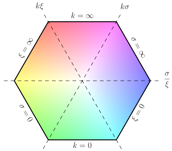
Figure 4: (Color online) Parameter space of the disordered Bogoliubov problem, spanned by three length scales: healing length $\xi$, excitation wave vector $k$, and disorder correlation length $\sigma$. At opposing vertices, the three dimensionless parameters $k\xi$, $k\sigma$, and $\sigma/\xi$ take their extreme values $0$ or $\infty$. On the six edges, one of the length scales itself is either $0$ or $\infty$.

These parameters are not independent, for any given two of them determine the third, e.g. $(k\sigma)/(k\xi)=\sigma/\xi$. The parameter space thus is a two-dimensional manifold. Nonetheless, it is useful to keep all three parameters to describe the various physical regimes. We have therefore found it convenient to map the entire parameter space to a hexagon, see Fig. 4. The three symmetry axes connecting the vertices carry the three dimensionless parameters, such that the extreme values $0$ and $\infty$ occur at opposite vertices. The symmetry axes perpendicular to the edges then represent the values of the length scales themselves, with their extreme values $0,\infty$ taken on the entire edges. This construction is analogous to the representation of RGB color space by hue and saturation at fixed lightness. Each of the three dimensionless parameters describes one of the channels, e.g. $k\xi$ the red channel with $k\xi=0$ mapped to cyan and $k\xi=\infty$ mapped to red. Similarly, $k\sigma$ and $\sigma/\xi$ define the green and blue channel, respectively, which completes the color space, as shown in Fig. 4.

IV Results

All of the physical quantities that we compute in the following depend crucially on the correlation parameter $\zeta=\sigma/\xi$ measuring the disorder potential correlation in units of the condensate healing length. In general, the results will even depend on the specific pair correlation function $C_{d}(k\sigma)$ defined in Eq. (77). For concreteness and direct applicability to cold-atom experiments, we will study in detail the case of optical speckle patterns, some properties of which are summarized in Sec. A. However, many analytical results in limiting cases are independent of the specific pair correlation and are thus universally applicable.

IV.1 Mean free paths

IV.1.1 Elastic scattering mean free path

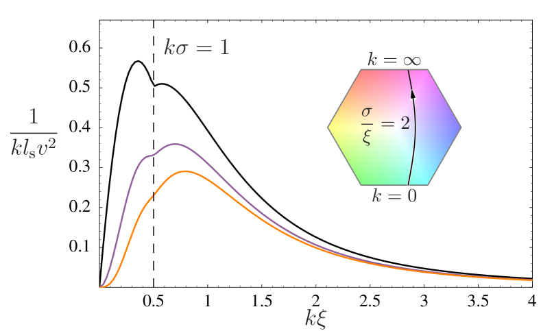
Figure 5: (Color online) Inverse elastic scattering mean free path (87) as function of Bogoliubov wave number $k\xi$ for disorder with fixed correlation parameter $\zeta=\sigma/\xi=2$, in $d=1,2,3$ dimensions (top to bottom). For small or large $k\xi$, universal limiting behavior is found, see text. The feature at $k\sigma=1$ is particular to the speckle disorder [Eq. (111)]. Inset: the plot’s path in the parameter space, Figure 4.

First, we evaluate the elastic scattering mean free path, in the dimensionless form $1/(kl_{\text{s}})=-2{\rm Im}\Sigma(k)/(\hbar kv_{\text{g}})$, which is the small parameter of weak-disorder expansions in standard quantum transport theories Rammer (1998). The only possibility for an imaginary part to occur in the on-shell self-energy (79) is by the imaginary part of the Green function, ${\rm Im}(\epsilon_{k}-\epsilon_{{\boldsymbol{k}}+{\boldsymbol{q}}}+i0)^{-1}=-\pi\delta(\epsilon_{k}-\epsilon_{{\boldsymbol{k}}+{\boldsymbol{q}}})$, multiplying the normal scattering amplitude. This restricts the integral over the intermediate state to the energy shell. There, the scattering element simplifies according to Eq. (36), and we find

$$\frac{1}{kl_{\rm s}}=\frac{\pi v^{2}}{2}\frac{k^{d}\sigma^{d}}{(1+k^{2}\xi^{2})^{2}}\int\frac{{\rm d}\Omega_{d}}{(2\pi)^{d}}A(k\xi,\theta)^{2}C_{d}\bigl{(}2k\sigma\sin\textstyle{\frac{\theta}{2}}\bigr{)}.$$ (87)

Fig. 5 shows this inverse scattering mean free path plotted as function of $k\xi$ for a speckle potential [Eq. (111)] with a fixed correlation ratio $\zeta=\sigma/\xi=2$ in dimensions $d=1,2,3$. The $k$-dependent fraction in front of the integral in (87) ensures that the mean free path diverges both for very low and high momenta, where one recovers essentially a clean system. In-between, around $k\xi=1$, there is a minimum mean free path. Fig. 5 also shows a feature at $k\sigma=1$, which is specific to the speckle correlation function used here, due to the non-analyticity at the boundary of its support. Indeed, in $d=1$, at this point the contribution of the backscattering process $k\to{-}k$ becomes impossible at the level of the Born approximation, which explains the kink at $k\sigma=1$. In higher dimensions, the angular integration lifts the singularity to higher derivatives, so that it becomes less conspicuous.

Obviously, the mean free path (87) depends on the two dimensionless parameters $k\xi$ and $k\sigma$. Let us discuss some interesting limiting cases, which are easily identified in our parameter space representation.

(i) First, the hydrodynamic limit $\xi\to 0$ is found on the lower right-hand edge of Fig. 4. Here, we recover exactly the elastic mean free path for scattering of sound waves Gaul et al. (2009), which only depends on the remaining parameter $k\sigma$.

(ii) Secondly, the limit $\xi\to\infty$ is found on the upper left-hand edge of Fig. 4. There, $\xi$ drops out together with the interaction energy $gn$ from (87), which reduces exactly to the elastic mean free path for single-particle scattering, as calculated in Kuhn et al. (2005, 2007). This reduced mean free path $kl_{\text{s}}$ can again only depend on $k\sigma$.

More generally, let us consider a fixed correlation ratio $\sigma/\xi$ of order unity, and look at the asymptotics as function of $k\xi$, as plotted in Fig. 5.

(iii) As $k\xi\to 0$, also $k\sigma\to 0$. Then, the potential correlator becomes isotropic, $C_{d}(2k\sigma\sin\frac{\theta}{2})\to C_{d}(0)$, and pulls out of the integral over $A(0,\theta)^{2}=\cos^{2}\theta$. This integral yields $\int\mathrm{d}\Omega_{d}\cos^{2}\theta=S_{d}/d$ (a result showing the “concentration of measure” of the hypersphere’s surface around its equator Milman and Schechtman (1986)). Thus, we obtain

$$\frac{1}{kl_{\text{s}}}=\frac{\pi S_{d}v_{\delta}^{2}}{2d(2\pi)^{d}}(k\xi)^{d}[1+O(k\xi,k\sigma)]$$ (88)

where $S_{d}$ is the unit sphere’s surface ($S_{1}=2$, $S_{2}=2\pi$, $S_{3}=4\pi$), and we define the effective $\delta$-correlation disorder strength

$$v_{\delta}^{2}=C_{d}(0)\frac{\sigma^{d}V^{2}}{\xi^{d}(gn)^{2}}.$$ (89)

The low-$k$ behavior $1/kl_{\text{s}}\propto(k\xi)^{d}$ indeed appears clearly in Fig. 5. In our parameter space Fig. 4, this is the asymptotic behavior of curves starting from the lower edge $k=0$, for intermediate values of $\sigma/\xi$, i.e. rather in the center of the edge. Note that $l_{\rm s}^{-1}\propto k^{d-1}$ is proportional to the surface of the energy shell, i.e. the number of states available for elastic scattering. In the limit $k\rightarrow 0$, the elastic energy shell shrinks and the scattering mean free path diverges, even when measured in units of $k^{-1}$.

(iv) Conversely, as $k\xi\to\infty$, also $k\sigma\to\infty$. But as soon as $k\sigma\gg 1$, the disorder potential allows practically only forward scattering, and we can make a small-angle approximation to all functions of $\theta$, such as $2k\sigma\sin{\frac{\theta}{2}}\to k\sigma\theta$. Then, the final result can be cast into the form

$$\frac{1}{kl_{\text{s}}}=\frac{V^{2}}{E_{\sigma}^{2}}\frac{f_{d}(\sigma/\xi)}{(k\sigma)^{3}}[1+O(1/k\xi,1/k\sigma)]$$ (90)

where $E_{\sigma}=\hbar^{2}/(m\sigma^{2})$ is the characteristic correlation energy Kuhn et al. (2005, 2007), and $f_{1}(\zeta)=C_{1}(0)$ as well as

$$f_{d}(\zeta)=S_{d-1}\int_{0}^{\infty}\frac{\mathrm{d}u\,u^{d-2}}{(2\pi)^{d-1}}\frac{(2\zeta^{2}-u^{2})^{2}}{(2\zeta^{2}+u^{2})^{2}}C_{d}(u)$$ (91)

in $d=2,3$. And indeed, all curves in Fig. 5 show this decrease as $k^{-3}$ for large momenta. In our parameter space Fig. 4, this is the asymptotic behavior of curves arriving at the upper edge $k=\infty$ for intermediate values of $\sigma/\xi$.

For extreme values of $\sigma/\xi$, i.e. towards the far left or right of the parameter space, one can also find interesting asymptotics when the wave length $2\pi/k$ lies between $\sigma$ and $\xi$.

(v) Consider first the case of a potential in the deep Thomas-Fermi regime $\sigma\gg\xi$ and excitations with $k\sigma\gg 1\gg k\xi$. This describes hydrodynamic excitations, i.e. a set of parameters approaching the right outermost vertex of Fig. 4 along the edge $\xi=0$. Then, by the same reasoning as in the previous case (iv), strongly peaked forward scattering leads to $1/kl_{\text{s}}\propto k\sigma$. This linear increase of the inverse scattering mean free path would naïvely predict infinitely strong scattering as $k$ increases. Within the full description, however, this unphysical behavior stops as soon as $k\xi\approx 1$ is reached, crossing over to case (iv) with an even simpler description since now $\zeta\gg 1$ for which $f_{d}(\infty)=S_{d-1}(2\pi)^{1-d}\int_{0}^{\infty}\mathrm{d}u\,u^{d-2}C_{d}(u)$ in $d=2,3$.

(vi) Conversely, consider finally a potential in the deep smoothing regime $\sigma/\xi\ll 1$ and excitations with $k\sigma\ll 1\ll k\xi$. This describes particle excitations, i.e. a set of parameters approaching the left outermost vertex of Fig. 4 along the edge $\xi=\infty$. Then, by the same reasoning as in case (iii), isotropic scattering leads to $1/kl_{\text{s}}\propto(k\sigma)^{d-4}$. This low-$k$ divergence of the scattering mean free path naïvely predicts infinitely strong scattering as $k\sigma\ll 1$ and severely limits the validity of simple perturbation theory for the single-particle case Kuhn et al. (2005, 2007). Not so here, where the divergence is avoided once $k\xi\approx 1$ is reached, and the interaction energy comes into play, crossing over to case (iii).

In summary, our perturbation theory provides valid expressions for the elastic scattering rate or inverse mean free path in the full space of parameters. At a given value of $\zeta=\sigma/\xi$, the scattering rate is always a bounded function of $k$, multiplied with the small parameter $v^{2}\ll 1$, which vindicates the use of the momentum basis as a starting point for the perturbation theory.

IV.1.2 Transport mean free path

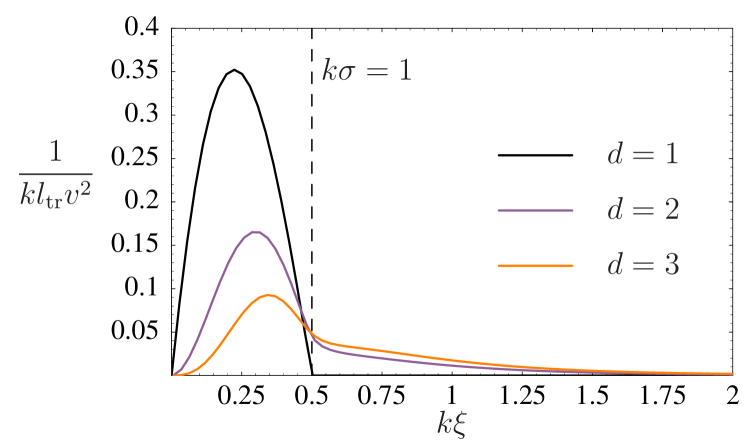
Figure 6: (Color online) Inverse transport mean free path, (87) including the vertex correction factor $(1-\cos\theta)$ under the integral, for a speckle disorder (111) with fixed correlation parameter $\zeta=\sigma/\xi=2$.

If a disordered BEC is brought out of equilibrium, it will respond via its excitations. Therefore, it is of interest to study the transport properties of Bogoliubov excitations. In principle, a full-fledged quantum transport theory requires to calculate particle-hole propagators, which is certainly doable using the Hamiltonian (62), but beyond the scope of the present article. Still, the previous results on the scattering mean free path can be generalized, with very limited additional effort, to the Boltzmann transport mean free path Kuhn et al. (2005, 2007) that measures the diffusive randomization of the direction of motion. This transport mean free path $l_{\text{tr}}$ is defined by the same integral expression (87), where the integrand is multiplied by a factor $(1-\cos\theta)$. Fig. 6 shows a plot of $1/kl_{\text{tr}}$ as function of $k\xi$ for a speckle disorder (111) with fixed correlation parameter $\zeta=\sigma/\xi=2$ in dimensions $d=1,2,3$.

In one dimension, the only contribution to the inverse transport mean free path is the backscattering contribution $k\to{-k}$, such that

$$\frac{1}{kl_{\text{tr}}}=\frac{v^{2}}{2}\frac{k\sigma\,C_{1}(2k\sigma)}{(1+k^{2}\xi^{2})^{2}}.$$ (92)

Due to the finite support of the speckle correlation function (111a) backscattering is impossible for $k\sigma>1$, and the inverse transport mean free path vanishes (within the Born approximation, and here we do not consider higher-order corrections to $l_{\text{tr}}$ Lugan et al. (2009); Gurevich and Kenneth (2009)), as clearly apparent from Fig. 6. In dimensions $d\geq 2$, there are finite contributions from small scattering angles. Adapting the reasoning of case (iv) from the previous section, one finds that $1/kl_{\text{tr}}\propto(k\sigma)^{-5}$, with a prefactor that can be determined similarly.

IV.1.3 Localization length

Just as phonons and particles, Bogoliubov excitations are expected to localize in disordered environments. Again, a full calculation is out of reach within the present article, but we can estimate the localization lengths of our Bogoliubov excitations in correlated disorder, based on general results on localization of particles and phonons.

In one-dimensional disordered systems, the localization length $l_{\text{loc}}=2l_{\text{tr}}$, which describes exponential localization, is directly proportional to the backscattering length that we just calculated Thouless (1973). From (92) we deduce

$$\frac{1}{kl_{\text{loc}}}=\frac{v^{2}}{4}\frac{k\sigma\,C_{1}(2k\sigma)}{(1+k^{2}\xi^{2})^{2}},$$ (93)

which agrees perfectly with Lugan et al. (2007), and also with Bilas and Pavloff (2006), in the limits $\sigma\rightarrow 0$ and $\xi\rightarrow 0$ investigated there. Those phase-formalism approaches are particularly suited for 1D systems, whereas our Green-function theory permits going to higher dimensions without conceptual difficulties.

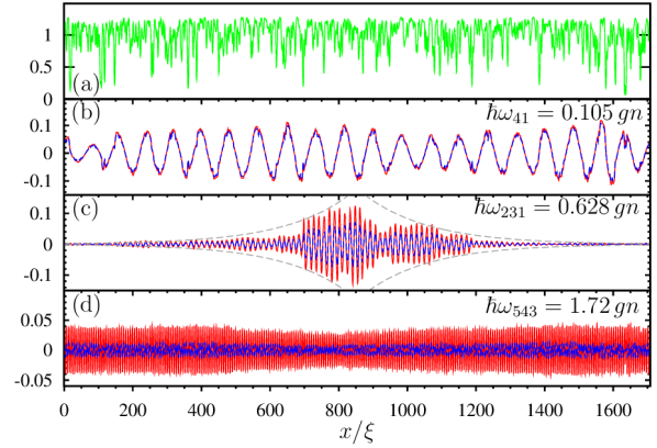
Figure 7: (Color online) (a) Condensate density $n(x)/n$ of a BEC (system size $L\approx 1700\xi$, periodic boundary conditions) in a blue-detuned speckle potential with amplitude $V/gn=0.3$ and correlation length $\sigma=\xi$. (b)–(d) Selected Bogoliubov modes $u_{\nu}(x)$ (solid red) and $v_{\nu}(x)$ (dashed blue), obtained by exact diagonalization of the Bogoliubov-de Gennes equation (50). Low- and high-energy modes [(b) and (d)] are extended, while localization is most pronounced at intermediate energies [(c)]. The dashed gray line in panel (c) shows the exponential envelope predicted by Eq. (93).

In two dimensions, the localization length is related to the transport mean free path via $l_{\text{loc}}=l_{\text{tr}}\exp\{\frac{\pi}{2}kl_{\text{tr}}\}$. This result can be derived using scaling theory arguments that hold very generally for single-particle excitations, and also the localization length of phonons has been shown to scale exponentially with $l_{\text{tr}}$ John et al. (1983).

In three dimensions, localized and delocalized states can coexist, as function of energy separated by a mobility edge. Phonons are localized at high energies and particles are localized at low energies John et al. (1983). These opposite characteristics imply that when the disorder is increased, localized modes will start to appear at energies close to the point where $l_{\text{tr}}$ is minimum.

So in all dimensions, localization will be observed most readily, within finite systems, for modes that have the shortest localization length. Our results on the transport mean-free path in correlated potentials show (in agreement with the 1D results of Lugan et al. (2007)) that modes around $k\xi=1$ will be the first to appear localized.

In one dimension, we have quantitatively verified the prediction (93) by means of an exact diagonalization of the inhomogeneous Bogoliubov-de Gennes equation (50), after solving the stationary GP equation (5) for the condensate. Fig. 7 shows that indeed only Bogoliubov modes at intermediate energies $\hbar\omega_{\nu}\approx 0.6gn$ appear localized in the finite system. The observed localization length is compatible with the prediction, Eq. (93).

All lengths calculated so far have the property that they diverge in the limit $k\xi\ll 1$. In other words, sound waves can propagate over long distances and for long times in these disordered systems. It is therefore meaningful to compute the renormalized speed of sound.

IV.2 Speed of sound

As shown in Sec. III.4, the disorder potential shifts the dispersion relation by $\Delta\overline{{\epsilon}}_{k}={\rm Re}\Sigma(k)$. Using Eqs. (83) and (79), the relative dispersion shift takes the form

$$\frac{\Delta\overline{{\epsilon}}_{k}}{\epsilon_{k}v^{2}}=\sigma^{d}\int\frac{{\rm d}^{d}q}{(2\pi)^{d}}z_{{\boldsymbol{k}}{\boldsymbol{q}}}C_{d}(q\sigma).$$ (94)

The kernel $z_{{\boldsymbol{k}}{\boldsymbol{q}}}$ obtains from the real part of the on-shell kernel $Z_{{\boldsymbol{k}}({\boldsymbol{k}}+{\boldsymbol{q}}){\boldsymbol{k}}}(\epsilon_{k})$, Eq. (78):

$$z_{{\boldsymbol{k}}{\boldsymbol{q}}}=\frac{(gn)^{2}}{\epsilon_{k}}\biggl{[}\operatorname{P}\frac{[w^{(1)}_{{\boldsymbol{k}}({\boldsymbol{k}}+{\boldsymbol{q}})}]^{2}}{\epsilon_{k}-\epsilon_{{\boldsymbol{k}}+{\boldsymbol{q}}}}-\frac{[y^{(1)}_{{\boldsymbol{k}}({\boldsymbol{k}}+{\boldsymbol{q}})}]^{2}}{\epsilon_{k}+\epsilon_{{\boldsymbol{k}}+{\boldsymbol{q}}}}+w^{(2)}_{{\boldsymbol{k}}({\boldsymbol{k}}+{\boldsymbol{q}}){\boldsymbol{k}}}\biggr{]},$$ (95)

with the envelopes defined in Eqs. (35a), (35b), and (42). $\operatorname{P}$ denotes the principal value. These equations reduce to much simpler expressions in different limiting regions of the parameter space, Fig. 4. We mostly focus on the low-energy, sound excitations that are of primary interest. Analytical results will be confronted with data from a numerical simulation in Sec. IV.2.2 below. At last, we show in Sec. IV.2.4 that our theory also covers the case of weak lattice potentials.

IV.2.1 Limiting cases

Similar to the proceeding in Sec. IV.1, we compute analytical results in the limiting cases located at the edges and corners of the parameter space, Fig. 4.

(i) We start with the hydrodynamic limit $\xi\to 0$, the lower right edge of Fig. 4. The kernel (95) simplifies to

$$-\frac{1}{2k^{2}}\operatorname{P}\frac{(k^{2}+{\boldsymbol{k}}\cdot{\boldsymbol{q}})^{2}}{q^{2}+2{\boldsymbol{k}}\cdot{\boldsymbol{q}}},$$ (96)

after which Eq. (94) reproduces exactly Eq. (29) of Ref. Gaul et al. (2009). Notably, the dispersion shift is negative in all dimensions and for any value of $\sigma/\xi\gg 1$, as anticipated in the schematic plot of Fig. 2(a). The limiting values are

$$\frac{\Delta\overline{{\epsilon}}_{k}}{\epsilon_{k}v^{2}}= -1/(2d), k\xi\ll k\sigma\ll 1$$ , (97a)

$$\frac{\Delta\overline{{\epsilon}}_{k}}{\epsilon_{k}v^{2}}= -(2+d)/8, k\xi\ll 1\ll k\sigma$$ . (97b)

These limiting values are expected to hold over an extended range of $k\sigma$. Thus, they define a shift in the local slope of the dispersion relation. In other words, $k$-modes in that particular range have a modified sound velocity. The magnitude of the correction depends significantly on the excitation’s ability to resolve the correlations ($k\sigma\gg 1$) or not ($k\sigma\ll 1$). As noted in Gaul et al. (2009), in the latter case the correction decreases with dimension, but increases in the former, implying that the curves for different dimensions must cross around $k\sigma=1$.

In passing, we stress that even in the very long-range correlated limit $\sigma/\xi\to\infty$, these results are not trivial. Indeed, one could try and use a simple static local density approximation (LDA) in order to derive the result (97b) for correlation lengths much longer than the excitation wave length. In this regime, the background appears locally homogeneous to the wave, and the local sound velocity $c({\boldsymbol{r}})=\sqrt{gn({\boldsymbol{r}})/m}$ is proportional to the condensate field amplitude $\Phi({\boldsymbol{r}})$. Thus, LDA expects $\Delta\overline{{c}}/c$ to be given by $\overline{{\Phi}}/\Phi$, which can be easily computed from Eq. (10) to yield $\Delta\overline{{c}}_{\rm LDA}/c=-v^{2}/8$. But this fails to reproduce Eq. (97b). Indeed, static LDA cannot capture the scattering dynamics (shown by the first diagram of Eq. (75)), which is essential for correctly determining the sound velocity.

(ii) In the regime of particle-like excitations $k\xi\to\infty$ (covering the cases (ii), (iv), and (vi) of Sec. IV.1), the Hamiltonian (1) becomes non-interacting. Consequently, one should expect the entire Bogoliubov problem to reduce to the problem of single particles in disorder. Indeed, Bogoliubov excitations in the particle regime see both, the external potential and the condensate background. Sampled at high wave numbers $k\xi\gg 1$, the condensate background is smooth and cannot induce scattering. Fittingly, we found in Sec. IV.1.1 that the elastic scattering mean free path reduces in this limit to the single-particle expression. In contrast, the deeply inelastic processes contributing to Eq. (94) remain sensitive to the condensate background, as encoded by the anomalous and second-order couplings, (35b) and (42), which do not simply vanish in the limit $\xi\to\infty$. We find that the leading-order correction to the dispersion relation (for $k\xi\gg 1$ and $k\sigma$ not too small),

$${\Delta\overline{{\epsilon}}_{k}}=v^{2}\sigma^{d}\int\frac{{\rm d}^{d}q}{(2\pi)^{d}}\frac{\epsilon_{q}^{0}C_{d}(q\sigma)}{(2+q^{2}\xi^{2})^{2}},$$ (98)

is independent of $k$. Incidentally, it is exactly opposite to the negative average shift $\overline{{\mu^{(2)}}}$ of the chemical potential, from Eq. (15), for fixed average density. At fixed chemical potential, the dispersion shift (98) would even be twice as big. Note that this shift cannot be naïvely accounted for by an overall shift $gn\to gn+\overline{{\mu^{(2)}}}$ in the clean dispersion, Eq. (25). Just like the wrong LDA attempt to explain the sound velocity, discussed above, such a reasoning misses the essential scattering dynamics.

Eq. (98) differs also from the chemical potential shift for noninteracting particles in disorder Bruus and Flensberg (2004). But it must be kept in mind that the disorder expansion of the Bogoliubov Hamiltonian in Sec. II.2.3 was performed under the assumption $V\ll gn$. For single particles, the interaction energy $gn$ goes to zero, i.e. the ratio of $V$ and $gn$ would have to be reversed. Therefore, our perturbative theory cannot be expected to apply universally in this regime.

In any case, the main effect of disorder in the single-particle regime is to yield the finite scattering rate calculated in Sec. IV.1, but it only produces a very small shift in dispersion. In addition, these high-energy excitations are less important for low-temperature properties of BECs, and will not be considered in the remainder of this work.

(iii) Let us turn to the sound-wave regime $k\xi\ll 1$. In case (i) and Ref. Gaul et al. (2009), this has been achieved by sending the healing length $\xi$ to zero, thus yielding the dispersion as function of $k\sigma$, but only for rather long-range correlated potentials with $\sigma\gg\xi$. In order to cover arbitrary correlation ratios $\zeta=\sigma/\xi$, we now change the point of view and take $k\to 0$. This allows in particular to reach the case $\sigma\ll\xi,k^{-1}$ of truly $\delta$-correlated disorder that was inaccessible to Gaul et al. (2009). The kernel (95) simplifies, and we find the relative shift in the speed of sound

$$\frac{\Delta\overline{{c}}}{cv^{2}}=\sigma^{d}\int\frac{{\rm d}^{d}q}{(2\pi)^{d}}\left\{\frac{2q^{2}\xi^{2}}{(2+q^{2}\xi^{2})^{3}}-\frac{2\cos^{2}\beta}{(2+q^{2}\xi^{2})^{2}}\right\}C_{d}(q\sigma).$$ (99)

$\beta=\measuredangle({\boldsymbol{k}},{\boldsymbol{q}})$ is the angle between the direction of propagation and ${\boldsymbol{q}}$. In contrast to the hydrodynamic case (i), there are now two competing contributions with opposite sign (for an interpretation of these contributions, cf. the end of Sec. IV.2.4 below). In case of isotropic correlation, the angular integral maps $\cos^{2}\beta$ to $1/d$. Then, only for $d=1$ is the radial integrand strictly negative, and $\Delta\overline{{c}}$ is negative as well. For $d>1$, the radial integrand has no definite sign.

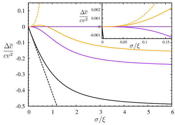
Figure 8: (Color online) Relative correction (99) of sound velocity due to a speckle disorder potential (111) as function of the correlation ratio $\zeta=\sigma/\xi$ in $d=1,2,3$. The exact formulae are given in Eq. (116). Dashed: universal limits, collected in Table 1. Inset: same data around the origin, showing the rapid departure from the leading-order estimate Giorgini et al. (1994); Lopatin and Vinokur (2002); Falco et al. (2007).

$\Delta\overline{{c}}/c$	$d=1$	$d=2$	$d=3$
$\sigma\gg\xi$	$-v^{2}/2$	$-v^{2}/4$	$-v^{2}/6$
$\sigma\ll\xi$	$-\frac{3}{16\sqrt{2}}v_{\delta}^{2}$	$0$	$+\frac{5}{48\sqrt{2}\pi}v_{\delta}^{2}$

Table 1: Limiting corrections of the speed of sound, corresponding to the dashed limits of Fig. 8. For uncorrelated disorder, the correction is proportional to $v_{\delta}^{2}$ of Eq. (89).

To survey the possible outcomes, we plot in Fig. 8 the correction (99) to the speed of sound caused by isotropic speckle disorder, Eq. (111), as function of the correlation ratio $\zeta=\sigma/\xi$. The curves can actually be given in closed form, see (116), but the details depend of course on the specific correlation. In contrast, we can extract universal limits for very small or very large $\zeta$.

In the long-range correlated limit $\zeta\to\infty$, found on the right edge of the plot, the correlator $C_{d}$ acts as a $\delta$-distribution, which leads to $\Delta\overline{{c}}/c=-v^{2}/(2d)$. This value coincides with the hydrodynamic limit (97a), as it should.

In the opposite limit $\zeta\ll 1$ of $\delta$-correlated disorder, the correlator $C_{d}(q\sigma)\to C_{d}(0)$ can be pulled out of the integral, which contributes a numerical prefactor to the expected scaling with the disorder strength $v_{\delta}^{2}$ defined in Eq. (89). These results are plotted as dashed lines in Fig. 8 and collected in Table 1. Again, these results cannot be found by LDA, which would have to assume that the system is homogeneous on relevant length scales ($\sigma\gg\xi,2\pi/k$), an assumption that is always violated by the sound-wave limit $2\pi/k\to\infty$.

Our result for $\sigma\ll\xi$ in $d=3$ reproduces the value known from Refs. Giorgini et al. (1994); Lopatin and Vinokur (2002); Falco et al. (2007). Interestingly, this is the only case where the correction to the speed of sound is positive. Actually, this particular numerical value is of rather limited use since the Taylor expansion at the origin is converging very slowly, and already a minor correlation can make a major difference, as shown by the inset in Fig. 8. Our results, Eqs. (94) and (99), hold for a much larger range of parameter values and arbitrary dimensions, which accomplishes one of the main goals of this work.

IV.2.2 Numerical mean-field study of the sound velocity

We confront the theoretical predictions (94) and (99) with data obtained by a numerical simulation in $d=1$ on the mean-field level, using the time-dependent Gross-Pitaevskii equation. This numerical calculation constitutes an independent check since it relies neither on the linearization in the excitations, nor on perturbation theory in the disorder potential, which are the two approximations of our analytical theory.

The numerical procedure has been briefly described in Ref. Gaul et al. (2009). We generate a 1D speckle disorder potential with correlation length $\sigma$ by Fourier transformation from the set of random complex field amplitudes [see Eq. (110)] with all $k\leq\sigma^{-1}$. Then the condensate ground state $\Phi(x)$ solving the GP equation (5) is computed by imaginary-time evolution, using the fourth-order Runge-Kutta algorithm, while keeping the wave function normalized Dalfovo and Stringari (1996). Onto this disordered ground state, a plane-wave Bogoliubov excitation is superposed, with a small, but finite $k$ and amplitude $\Gamma$. In cold-atom experiments, such an excitation is routinely imprinted using Bragg spectroscopy Stamper-Kurn et al. (1999); Vogels et al. (2002); Steinhauer et al. (2002, 2003). The Bogoliubov transformation (20) requires the imprints in density and phase to be

$$\delta n(x) =2\sqrt{n}a_{k}\,\Gamma\cos(kx), \delta\varphi(x) =\frac{\Gamma}{\sqrt{n}a_{k}}\sin(kx).$$ (100)

In the sound-wave regime where $a_{k}\ll 1$ [cf. Eq. (23)], the phase modulation has a much larger amplitude than the density modulation, and we choose $\Gamma=0.3\sqrt{n}a_{k}v$. Then, the real-time evolution under the GP equation is computed using again the fourth-order Runge-Kutta algorithm. The excitation propagates, with a modified speed of sound, surviving over a long course of time given by the inverse elastic scattering rate $\gamma_{k}^{-1}$ [cf. Eq. (82)]. In order to extract the eigenenergy $\epsilon_{k}$, the deviation $\delta\Phi(x,t)$ from the ground state is translated into Bogoliubov excitations by means of Eq. (20). Monitoring the phase of $\gamma_{k}\propto e^{-i\epsilon_{k}t/\hbar}$ over time, we extract the phase velocity $v_{\text{ph}}=\epsilon_{k}/\hbar k$ by linear regression. Then, the procedure is repeated for different realizations of disorder with the same correlation length $\sigma$, leading to a whole distribution of values, from which we compute the average $\Delta\overline{{c}}/c$. As shown in Ref. Gaul et al. (2009), for weak disorder the distribution is clearly single-peaked and allows for meaningful averages.

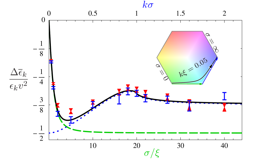
Figure 9: (Color online) Relative correction of the Bogoliubov excitation dispersion relation due to 1D speckle disorder. The full formula (94) for $k\xi=0.05$ [solid black] crosses over from the limiting case (iii) of low-energy excitations [dashed green, Eq. (116a)] to the limiting case (i) of the hydrodynamic regime [dotted blue, Eq. (112)]. The inset shows the corresponding trajectory in parameter space. The numerical results (cf. Sec IV.2.2) for blue- and red-detuned speckle with $v=+0.03$ [blue lines] and $v=-0.03$ [red triangles], agree fully with the analytical theory.

Figure 9 shows the numerical data on top of the theoretical predictions, as function of $\sigma$. Since $k\xi=0.05$ is fixed, the curve can be read as a function of $k\sigma$ at very small $\xi$ (near the hydrodynamic limit (i) of above) or as a function of $\sigma/\xi$ at very small $k$ (near the low-energy limit (iii) of above). The inset of Fig. 9 depicts the corresponding trajectory in parameter space. The full prediction (94) for $k\xi=0.05$ is plotted as a black line. The limiting cases are available in closed form: Eq. (112) for ${\xi=0}$ as function of $k\sigma$ and Eq. (116a) for ${k=0}$ as function of $\sigma/\xi$. Independently of the details, we find of course the relevant universal limits of Sec. IV.2.1 above.

The numerical data, shown for $v=+0.03$ (blue straight marks) and $v=-0.03$ (red triangular marks), follow the analytical prediction very well. Interestingly, the data points of red and blue detuning, with opposite sign of $v$, tend to lie on opposite sides of the curve, indicating beyond-Born effects of odd order $v^{3}$, which are expected for a speckle potential with its asymmetric on-site distribution (107). Attentive readers will also notice that the data points are shifted asymmetrically with respect to the curve, which is an effect of order $v^{4}$.

IV.2.3 Disorder-shift of Bogoliubov spectrum

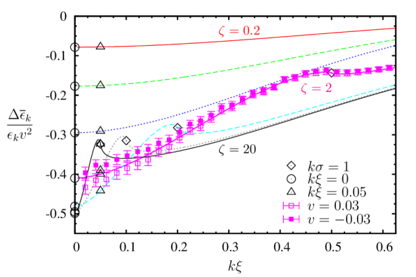
Figure 10: (Color online) Relative correction (94) of the dispersion relation $\Delta\overline{\epsilon}_{k}$ for different correlation ratios $\zeta=\sigma/\xi=0.2,0.5,1,2,5,10,20$ (top to bottom), for 1D speckle disorder, Eq. (111a). The results of Figure 8 appear at the edge $k\xi=0$ (circles), whereas the results shown in Figure 9 are found at $k\xi=0.05$ (triangles). Around the points $k\sigma=1$ (diamonds), the correction behaves non-monotonically. The points with errorbars close to the curve $\zeta=2$ show data from the exact diagonalization of the Bogoliubov-de Gennes eq. (50) (system size $L\approx 300\xi$, correlation $\sigma=2\xi$) for blue- as well as red-detuned speckle disorder. Each point represents the energy shift of the two modes $\nu=2j-1,2j$ corresponding to the degenerate modes $k_{j}=\pm 2\pi j/L$ of the homogeneous system. The data has been averaged over a large number $r$ of realizations ($rL/\sigma\approx 1.9\times 10^{4}$). Errorbars show the estimated error of the mean value.

Finally, we explore the correction of the dispersion relation (94) as function of $k\xi$. Figure 10 shows a family of curves for different correlation parameters $\zeta=\sigma/\xi$ in one dimension. This plot actually contains the information of the previous Figs. 8 and 9, which are taken at fixed values of $k\xi=0$ and $k\xi=0.05$, respectively.

The disorder correction passes through a non-monotonic feature around $k\sigma=1$ (marked by open diamonds), and finally diminishes with increasing $k\xi$.

In dimensions $d>1$, the curves have a slightly different shape. The curve with $\zeta=20$, for example, starts with the limit Eq. (97a) at $k\xi\to 0$ and passes through Eq. (97b) at $k\xi\approx 0.15$. Thus, while the 1D curve starts at $-1/2$ and passes through $-3/8$, the corresponding curve in $d=3$ will start at $-1/6$ and pass through an extremum around $-5/8$, before diminishing in the particle regime. Also, the sharp speckle features get washed out in higher dimensions.

Complementary to the previous numerical study at constant $k\xi$, we can verify our predictions also by an exact diagonalization of the one-dimensional disordered Bogoliubov-de Gennes equation (50). Thus, we obtain the whole spectrum of the system characterized by its correlation ratio $\zeta=\sigma/\xi$. For the case $\zeta=2$, Fig. 10 shows excellent agreement between prediction and numerics. As observed previously, the data for red- and blue-detuned speckle lie to both sides of the $O(v^{2}$) prediction, indicating effects of odd orders.

The excellent agreement between both numerical approaches and analytics demonstrates that our perturbation theory to order $v^{2}$ gives an impressive account of all relevant effects over the entire parameter space we set out to cover.

IV.2.4 Weak lattice potentials

The inhomogeneous Bogoliubov Hamiltonian (62) applies to arbitrary external potentials. In particular, it covers the important class of weak optical lattice potentials that was studied in Liang et al. (2008); Taylor and Zaremba (2003). In a sense, understanding the lattice is a first step to understanding disorder, which can be seen, by virtue of Fourier decomposition, as a superposition of lattices with suitably chosen random amplitudes and phases.

To substantiate this connection, we briefly show that our formalism reproduces the results of Liang et al. (2008); Taylor and Zaremba (2003) for the speed of sound in weak lattices. In $d$ dimensions, a separable lattice potential $V({\boldsymbol{r}})=\sum_{j=1}^{d}V_{j}\cos(K_{j}x_{j})$ with wave vectors ${\boldsymbol{K}}_{j}=K_{j}\hat{\boldsymbol{e}}_{j}$ has Fourier components

$$V_{\boldsymbol{q}}=\frac{1}{2}\sum_{j=1}^{d}V_{j}[\delta_{{\boldsymbol{q}}{\boldsymbol{K}}_{j}}+\delta_{{\boldsymbol{q}}(-{\boldsymbol{K}}_{j})}].$$ (101)

The whole formalism developed in Secs. II and III applies also to this potential. Notably, the equation of motion (67) is still solved by the perturbative expansion (73), now without the need for averaging over disorder. The periodic potential scatters Bogoliubov excitations elastically only at the edges of the Brillouin zone, $k_{j}=\pm K_{j}$. Away from the edges, the dispersion relation is again determined by the diagonal elements of the Green function $G(\epsilon)_{{\boldsymbol{k}}{\boldsymbol{k}}}$. Expressions like (79) and (94) are still valid, where the correlator should now be understood to stand for

$$V^{2}\sigma^{d}C_{d}(q\sigma)=\frac{(2\pi)^{d}}{4}\sum_{j=1}^{d}V_{j}^{2}\left[\delta({\boldsymbol{q}}-{\boldsymbol{K}}_{j})+\delta({\boldsymbol{q}}+{\boldsymbol{K}}_{j})\right].$$ (102)

In the sound-wave limit $k\to 0$, the speed-of-sound correction (99) thus reads

$$\frac{\Delta c}{c}=\sum_{j=1}^{d}\left\{\frac{K_{j}^{2}\xi^{2}}{(2+K_{j}^{2}\xi^{2})^{3}}-\frac{\cos^{2}\beta_{j}}{(2+K_{j}^{2}\xi^{2})^{2}}\right\}\frac{V_{j}^{2}}{(gn)^{2}}$$ (103)

where $\beta_{j}$ is the angle between the propagation direction and the lattice direction $\hat{\boldsymbol{e}}_{j}$. In the case $V_{2}=V_{3}=0$, the sound velocity along the $x_{1}$ direction reproduces the result of Ref. (Taylor and Zaremba, 2003, Eq. (52)). Also, Eq. (103) is precisely Eq. (22) in Ref. Liang et al. (2008) for the potential (102). This work of Liang et al. Liang et al. (2008), while equivalent to ours as far as the perturbative approach is concerned, has the nice feature that it permits to attach a thermodynamic meaning to the two antagonistic contributions appearing in Eq. (103): the first, positive term stems from the disorder-shift of the compressibility $\kappa$, while the second, negative one goes back to the change in the effective mass $m^{*}$. Together, these quantities determine the speed of sound $c=1/\sqrt{\kappa m^{*}}$.

IV.3 Average density of states

Lastly, we turn to the average density of states (AVDOS), Eq. (84), at very low energies or $k\to 0$. As shown above, the dispersion is linear in this limit, so that the AVDOS $\overline{{\rho}}(\epsilon)=\int\frac{{\rm d}^{d}k}{(2\pi)^{d}}\delta(\epsilon-\hbar\overline{{c}}k)=\rho(\epsilon)(c/\overline{{c}})^{d}$ necessarily has the lowest-order correction

$$\frac{\Delta\overline{{\rho}}(0)}{\rho(0)}=-d\frac{\Delta\overline{{c}}}{c}.$$ (104)

In other words, a reduced sound velocity entails an enhanced density of states and vice versa, which is the obvious conclusion one can already draw from the schematic plot anticipated in Fig. 2. It is instructive to check that identity (104) also follows from the general equation (85): There, the linear dispersion implies $k\partial_{k}\epsilon_{k}=\epsilon_{k}$, and the fraction approaches $\Delta\overline{{\epsilon}}_{k}/\epsilon_{k}$. When acting on this regular function, the operator $k\partial_{k}$ inside the bracket evaluates to zero at $k=0$, and we arrive at (104). Thus, the AVDOS shift is entirely determined by the sound velocity shift (99); see also the analytic solutions (116).

In the hydrodynamic regime $k\xi\ll 1$ realized by $\xi\to 0$ at finite $k\sigma$, again $k\partial_{k}\epsilon_{k}=\epsilon_{k}=\hbar ck$ in Eq. (85), which then reproduces our previous results Gaul et al. (2009). The limiting values for small or large energy compared to the hydrodynamic correlation energy $\hbar c/\sigma$, corresponding to (97), are

$$\frac{\Delta\overline{{\rho}}(\epsilon)}{\rho(\epsilon)}=\frac{v^{2}}{2}\times\begin{cases}1,&\epsilon\ll\hbar c/\sigma,\\ \frac{d}{4}(2+d),&\epsilon\gg\hbar c/\sigma.\end{cases}$$ (105)

In between these limits, the correction $\Delta\overline{{\rho}}/\rho$ as function of $\epsilon$ can show a surprisingly rich behavior, depending on the potential correlations. In three dimensions, the correction is smooth and monotonic, but in one dimension, speckle correlations are responsible for an unexpected, non-monotonic behavior with a sharp feature at $k_{\epsilon}\sigma=1$, as discussed in Gaul et al. (2009).

Note that these simple perturbative results are indeed expected to hold at low energy or $k\xi\ll 1$, in stark contrast to the case of single particles in disorder, where the DOS has a (nonperturbative) Lifshitz tail at low energy Lifshitz et al. (1988); Lugan et al. (2007). In the present case, the interparticle repulsion screens the disorder very effectively at low energy, such that localization effects are absent (cf. the diverging localization length of Sec. IV.1.3) Lee and Gunn (1990); Lugan et al. (2007). A transition to the Bose glass phase Giamarchi and Schulz (1987); *Giamarchi1988; Fisher et al. (1989) occurs only for stronger disorder or much weaker interaction, where the Bogoliubov theory developed here breaks down, and different approaches are needed Falco et al. (2009); Pilati et al. (2009); Carrasquilla et al. (2010).

V Conclusions and Outlook

In conclusion, we have formulated a comprehensive Bogoliubov theory of inhomogeneous Bose-Einstein condensates. This analytical theory describes the elementary excitations of condensates with s-wave interaction, deformed by weak external potentials with arbitrary spatial correlations and in arbitrary spatial dimension. Expanding the many-body Hamiltonian around the deformed ground state, we have obtained the inhomogeneous Bogoliubov Hamiltonian. We have justified our choice of the basis of density and phase fluctuations that ensures proper orthogonality between the excitations and the inhomogeneous Bogoliubov vacuum. Expressed in terms of Nambu-Bogoliubov spinors, all effects of the external potential can be collected into a scattering vertex that is non-perturbative in the external potential. A fully analytical formulation has been achieved up to second order in weak potentials, allowing in principle an expansion to even higher orders.

From this fundamental Hamiltonian, one can derive numerous physically relevant quantities by means of standard perturbation theory. This paper has been devoted to a detailed discussion of the single-excitation dispersion relation. We have calculated the mean-free path and renormalized speed of sound together with the resulting average density of states, over the full parameter space of the disordered Bogoliubov problem, with numerous analytical results in limiting cases. It turns out that the frequently investigated case of $\delta$-correlated disorder in three dimensions, with its positive shift in the speed of sound, is far from generic. Over most of the parameter space, the speed of sound is reduced. We have confirmed these predictions in detail by mean-field numerical simulations as well as exact diagonalization for the experimentally relevant case of correlated speckle disorder in $d=1$.

Strictly speaking, the present work is incomplete without proving that the weak disorder under consideration causes only a small condensate depletion. Indeed, the Bogoliubov ansatz (3) relies on the macroscopic population of the condensate mode. In a pure mean-field description, all atoms are in the condensate at zero temperature. But due to the effect of interaction, even at zero temperature, there is a finite fraction of particles not in the condensate, which constitutes the so-called quantum depletion that can be calculated within Bogoliubov theory Pethick and Smith (2002); Pitaevskii and Stringari (2003). The quantum depletion should be small, thus providing an important, self-consistent check of the theory’s validity.

In the homogeneous setting, the mean-field condensate forms in the homogeneous mode, i.e., the zero-momentum state. Thus, the quantum depletion consists of all particles with non-zero momentum. The density of these particles can be easily calculated within Bogoliubov theory Pethick and Smith (2002); Pitaevskii and Stringari (2003), with the result (we take $d=3$ here) that the fractional quantum depletion $\delta n/n=8(na_{\rm s}^{3})^{1/2}/3\sqrt{\pi}$ is proportional to the root of the gas parameter and thus very small, especially so for dilute and weakly interacting cold gases.

It is not immediately obvious how to generalize the recipe “count all particles with non-zero momentum” to the inhomogeneous case. The vast majority of works dedicated to the inhomogeneous Bogoliubov problem simply calculates the same quantity, namely the number of particles with non-zero momentum. But one has no means of knowing whether these particles belong to the deformed condensate or to the true, disorder-induced quantum depletion. And really, the supposed “depletion” calculated by Huang and Meng, followed by Huang and Meng (1992); Giorgini et al. (1994); Astrakharchik et al. (2002); Kobayashi and Tsubota (2002), involves only the condensate deformation at fixed chemical potential, which is a mean-field effect as described in Sec. II.1. Only few authors seem to have clearly recognized that this supposed depletion describes merely the non-uniform density of the condensate Lopatin and Vinokur (2002).

In order to assess the true condensate depletion, one has to determine the density of particles not in the condensate at all, irrespective of their particular momentum. With the general Bogoliubov Hamiltonian at hand, we have calculated this disorder-induced quantum depletion Gaul and Müller (2010). We find that it is much smaller than the mean-field condensate deformation. This is no surprise: To first order, the external potential merely deforms the condensate. The scattering of particles out of the condensate is a second-order effect, mediated by the interaction between particles and the condensate. Details of the full calculation, including finite-temperature effects, will be discussed in a forthcoming publication Müller and Gaul (2011).

These results validate and strengthen the Bogoliubov approach, and we expect that the theory we have developed here should fare very well in describing the excitations of inhomogeneous BECs. As an immediate extension of the present work, finite-temperature effects can be captured very straightforwardly by the Matsubara formalism Bruus and Flensberg (2004), allowing the calculation of the heat capacity and many other (thermo-)dynamic response functions. This is left for future work.

Appendix A Optical speckle disorder

A.1 Statistical properties

The optical speckle field of a laser defines a disorder potential with very well controlled statistical properties Goodman (1975); Clément et al. (2006); Lugan et al. (2009); Sanchez-Palencia and Lewenstein (2010). When coherent laser light is directed on a rough surface or through a diffusor plate, the elementary waves originating from different points have random phases and form a random interference pattern in the far field. By virtue of the central limit theorem, the resulting field $\mathcal{E}({\boldsymbol{r}})$ is a complex Gaussian random process. For notational simplicity, we consider a scalar field with dipole coupling to a single atomic transition and neglect polarization issues. The electronic atomic ground state is then subject to the light-shift potential induced by the intensity $I({\boldsymbol{r}})=|\mathcal{E}({\boldsymbol{r}})|^{2}$ Grimm et al. (2000). Magnitude and sign of this potential depend on the laser detuning from the dipole transition frequency. For a far-detuned potential, one has

$$V({\boldsymbol{r}})=V\left(\frac{I({\boldsymbol{r}})}{I_{0}}-1\right),$$ (106)

The prefactor $V$ contains the atomic polarizability, besides all other proportionality factors, and we have shifted the potential to zero average, $\overline{{V({\boldsymbol{r}})}}=0$. The magnitude of $V$ gives the variance of the potential fluctuations, $V^{2}=\overline{{V({\boldsymbol{r}})^{2}}}$, that can be readily adjusted in the experiment by changing the overall laser intensity. Because the intensity is the modulus square of the Gaussian field $\mathcal{E}$, the potential has a skewed on-site probability distribution for $w=V({\boldsymbol{r}})/V$,

$$P(w){\rm d}w=\Theta(w+1)e^{-(w+1)}{\rm d}w.$$ (107)

A blue-detuned potential with $V>0$ consists of high potential bumps rising over a flat baseline. A red-detuned potential with $V<0$ rather corresponds to a random set of deep wells.

The potential correlation between different spatial points is captured by the pair correlator

$$\widehat{C}_{d}(r/\sigma)=\overline{{V({\boldsymbol{r}})V(0)}}/V^{2}$$ (108)

that decays from the starting value $\widehat{C}_{d}(0)=1$ to zero on the scale of the correlation length $\sigma$. In momentum representation, the normalization implies the useful identity

$$\int\frac{{\rm d}^{d}(q\sigma)}{(2\pi)^{d}}C_{d}(q\sigma)=1.$$ (109)

A speckle pattern’s correlation is entirely determined by the fact that the Fourier components of the field $\mathcal{E}_{\boldsymbol{k}}$ are independent, complex Gaussian random variables with a pair correlation

$$\overline{{\mathcal{E}_{\boldsymbol{k}}^{*}\mathcal{E}_{{\boldsymbol{k}}^{\prime}}}} =:\gamma(k)\delta_{{\boldsymbol{k}}{\boldsymbol{k}}^{\prime}}$$ (110)

that defines the degree of coherence $\gamma(k)$. In one dimension, for a rectangular source, the degree of coherence $\gamma(k)=\gamma\Theta(1-k\sigma)$ Kuhn et al. (2007) has uniform weight inside the interval of allowed $k$-values. The correlation length $\sigma$ depends on the laser wave length and the imaging optics and is typically of the order of $1\,\mu$m or smaller Billy et al. (2008). It is not easy to create an isotropic multi-dimensional speckle field in the laboratory Robert-de-Saint-Vincent et al. (2010). For the purpose of the present paper, we follow Pilati et al. Pilati et al. (2009) and define the isotropic speckle disorder on the grounds of Eq. (110) with the same $\gamma(k)$ in all dimensions. This definition grasps the essential feature of speckle disorder, namely the finite support of its power spectrum. The extension to a more realistic, possibly anisotropic correlation function for a given experimental configuration is straightforward within the present formalism.

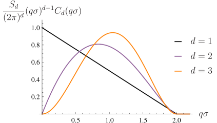
Figure 11: Isotropic speckle correlation function as function of reduced momentum in $d=1,2,3$. In order to show comparable scales, we plot $[S_{d}/(2\pi)^{d}](q\sigma)^{d-1}C_{d}(q\sigma)$, including the $d$-dimensional volume integration element.

The potential correlator $C_{d}(k\sigma)$, used in Eq. (77) and the following, then obtains as the auto-convolution of the field correlator $\gamma(k)$, i.e. of a $d$-dimensional ball of radius $\sigma^{-1}$. Thus, $C_{d}(q\sigma)$ is centered at $q=0$ and vanishes like $(2-q\sigma)^{\smash{\frac{d+1}{2}}}$ at $q=2\sigma^{-1}$. Explicitly, in $d=1,2,3$ one has

$$C_{1}(q\sigma) =\frac{\pi}{2}(2-q\sigma)\,\Theta(2-q\sigma),$$ (111a)

$$C_{2}(q\sigma) =\left[8\arccos\left(\textstyle{\frac{q\sigma}{2}}\right)-2q\sigma\sqrt{4-q^{2}\sigma^{2}}\right]\Theta(2-q\sigma),$$ (111b)

$$C_{3}(q\sigma) =\frac{3\pi^{2}}{8}(2-q\sigma)^{2}(4+q\sigma)\,\Theta(2-q\sigma).$$ (111c)

Figure 11 shows these isotropic correlation functions, multiplied with the $d$-dimensional integration element $S_{d}(q\sigma)^{d-1}/(2\pi)^{d}$, where $S_{d}$ is the unit-sphere surface ($S_{1}=2$, $S_{2}=2\pi$, $S_{3}=4\pi$).

A.2 Analytical dispersion corrections

The speckle correlation functions (111) yield closed-form expressions for the dispersion correction (94) in important limiting cases.

A.2.1 Hydrodynamic limit $\xi=0$

In $d=1$, the correlation function (111a) is piecewise linear, and the integral (94) over the hydrodynamic kernel (96) yields the dispersion shift Gaul et al. (2009); Renner (2009)

$$\frac{\Delta\overline{{\epsilon}}_{k}}{\epsilon_{k}v^{2}} =-\frac{1}{2}-\frac{k\sigma}{8}\ln\left|\frac{1-k\sigma}{1+k\sigma}\right|+\frac{k^{2}\sigma^{2}}{8}\ln\left|\frac{1-k^{2}\sigma^{2}}{k^{2}\sigma^{2}}\right|.$$ (112)

This result is plotted as the blue dotted curve in Figure 9. It is non-analytic at $k\sigma=1$, corresponding to the non-analyticity of the speckle pair correlation function (111a) at the boundary of its support. Using Eq. (112), we can also write down the AVDOS shift (85) in closed form:

$$\frac{\Delta\overline{{\rho}}(\varepsilon\hbar c/\sigma)}{\rho(\varepsilon\hbar c/\sigma)v^{2}}=\frac{1}{2}+\frac{\varepsilon}{4}\ln\left|\frac{1-\varepsilon}{1+\varepsilon}\right|-\frac{3\varepsilon^{2}}{8}\ln\left|\frac{1-\varepsilon^{2}}{\varepsilon^{2}}\right|.$$ (113)

It shows a pronounced dip around $\varepsilon\approx 0.7$ and a sharp logarithmic divergence at $\varepsilon=1$ Gaul et al. (2009), resulting from the non-analyticity of (113) at $k\sigma=1$.

In higher dimensions, the integral (94) gets more complicated, but we find partial analytical results in two dimensions. Denote the angular part of the integral (94) over the hydrodynamic kernel (96) by $A_{2}(q)$. We drop the principal value $\operatorname{P}$ in Eq. (96) and re-insert the infinitesimal imaginary shift in the denominator. Then, we can compute the angular integral analytically as a closed-path integral in the complex plane $z=e^{i\beta}$, $\beta=\measuredangle({\boldsymbol{k}},{\boldsymbol{q}})$

$$A_{2}(q)=-\frac{1}{2}\frac{S_{2}}{(2\pi)^{2}}\left[1-\left(\frac{q}{2k}\right)^{2}+k^{2}\frac{1-{q^{2}}/(2k^{2})}{q\sqrt{q^{2}-(2k)^{2}}}\right].$$ (114)

In general, the last term is too complicated for the remaining radial integral to be evaluated in closed form. For $k\sigma>1$, however, the integrand of Eq. (94) is restricted to $q\leq 2/\sigma<2k$. There, the last term in (114) is imaginary and does not contribute to ${\rm Re}\Sigma$, such that

$$\frac{\Delta\overline{{\epsilon}}_{k}}{\epsilon_{k}}=-\frac{v^{2}}{2}\left(1-\frac{1}{8k^{2}\sigma^{2}}\right),\quad k\sigma>1.$$ (115)

In the AVDOS (85), this leads to a totally flat plateau, as shown in Fig. 5 of Ref. Gaul et al. (2009).

A.2.2 Lowest-energy excitations, $k\to 0$

Also in the low-energy limit (iii) of Sec. IV.2.1, we can find analytical solutions. The integral (99) with the speckle correlator (111) evaluates to closed form in all relevant dimensions:

$$\frac{\Delta\overline{{c}}}{cv^{2}} =-\frac{3}{8}z\left[\cot^{-1}\big{(}z\big{)}+\frac{1}{3}\frac{z}{1+z^{2}}\right], d=1$$ (116a)

$$\frac{\Delta\overline{{c}}}{cv^{2}} =z^{3}\frac{2z\sqrt{1+z^{2}}-1-2z^{2}}{\sqrt{1+z^{2}}}\,, d=2$$ (116b)

$$\frac{\Delta\overline{{c}}}{cv^{2}} =z^{4}\biggl{[}7+\frac{5\cot^{-1}(z)}{2z}-(6+7z^{2})\log \left(\frac{1+z^{2}}{z^{2}}\right)\biggr{]},$$

$$d=3$$ (116c)

with $z=\zeta/\sqrt{2}$. All three cases are plotted in Figure 8; the result (116a) also features in Figure 9.

References

- Giamarchi and Schulz (1987) T. Giamarchi and H. J. Schulz, Europhys. Lett., 3, 1287 (1987).
- Giamarchi and Schulz (1988) T. Giamarchi and H. J. Schulz, Phys. Rev. B, 37, 325 (1988).
- Fisher et al. (1989) M. P. A. Fisher, P. B. Weichman, G. Grinstein, and D. S. Fisher, Phys. Rev. B, 40, 546 (1989).
- Crooker et al. (1983) B. C. Crooker, B. Hebral, E. N. Smith, Y. Takano, and J. D. Reppy, Phys. Rev. Lett., 51, 666 (1983).
- Chan et al. (1988) M. H. W. Chan, K. I. Blum, S. Q. Murphy, G. K. S. Wong, and J. D. Reppy, Phys. Rev. Lett., 61, 1950 (1988).
- Wong et al. (1990) G. K. S. Wong, P. A. Crowell, H. A. Cho, and J. D. Reppy, Phys. Rev. Lett., 65, 2410 (1990).
- Clément et al. (2005) D. Clément, A. F. Varón, J. A. Retter, P. Bouyer, L. Sanchez-Palencia, D. Gangardt, G. V. Shlyapnikov, and A. Aspect, Phys. Rev. Lett., 95, 170409 (2005).
- Schulte et al. (2005) T. Schulte, S. Denkelforth, J. Kruse, W. Ertmer, J. Arlt, K. Sacha, J. Zakrzewski, and M. Lewenstein, Phys. Rev. Lett., 95, 170411 (2005).
- Lye et al. (2005) J. E. Lye, L. Fallani, M. Modugno, D. S. Wiersma, C. Fort, and M. Inguscio, Phys. Rev. Lett., 95, 070401 (2005).
- Chen et al. (2008) Y. P. Chen, J. Hitchcock, D. Dries, M. Junker, C. Welford, and R. G. Hulet, Phys. Rev. A, 77, 033632 (2008).
- White et al. (2009) M. White, M. Pasienski, D. McKay, S. Q. Zhou, D. Ceperley, and B. DeMarco, Phys. Rev. Lett., 102, 055301 (2009).
- Dries et al. (2010) D. Dries, S. E. Pollack, J. M. Hitchcock, and R. G. Hulet, Phys. Rev. A, 82, 033603 (2010).
- Bogoliubov (1947) N. N. Bogoliubov, Journal of Physics (Moscow), 11, 23 (1947).
- Nozières and Pines (1999) P. Nozières and D. Pines, The Theory of Quantum Liquids (Perseus Books, Cambridge, MA, 1999).
- Lee and Gunn (1990) D. K. K. Lee and J. M. F. Gunn, J. Phys.: Condens. Matter, 2, 7753 (1990).
- Huang and Meng (1992) K. Huang and H.-F. Meng, Phys. Rev. Lett., 69, 644 (1992).
- Giorgini et al. (1994) S. Giorgini, L. Pitaevskii, and S. Stringari, Phys. Rev. B, 49, 12938 (1994).
- Kobayashi and Tsubota (2002) M. Kobayashi and M. Tsubota, Phys. Rev. B, 66, 174516 (2002).
- Astrakharchik et al. (2002) G. E. Astrakharchik, J. Boronat, J. Casulleras, and S. Giorgini, Phys. Rev. A, 66, 023603 (2002).
- Bilas and Pavloff (2006) N. Bilas and N. Pavloff, Eur. Phys. J. D, 40, 387 (2006).
- Lugan et al. (2007) P. Lugan, D. Clément, P. Bouyer, A. Aspect, and L. Sanchez-Palencia, Phys. Rev. Lett., 99, 180402 (2007a).
- Falco et al. (2007) G. M. Falco, A. Pelster, and R. Graham, Phys. Rev. A, 75, 063619 (2007).
- Fontanesi et al. (2009) L. Fontanesi, M. Wouters, and V. Savona, Phys. Rev. Lett., 103, 030403 (2009).
- Hu et al. (2009) Y. Hu, Z. Liang, and B. Hu, Phys. Rev. A, 80, 043629 (2009).
- Lewenstein et al. (2007) M. Lewenstein, A. Sanpera, V. Ahufinger, B. Damski, A. Sen, and U. Sen, Adv. Phys., 56, 243 (2007).
- Bloch et al. (2008) I. Bloch, J. Dalibard, and W. Zwerger, Rev. Mod. Phys., 80, 885 (2008).
- Sanchez-Palencia and Lewenstein (2010) L. Sanchez-Palencia and M. Lewenstein, Nat. Phys., 6, 87 (2010).
- Modugno (2010) G. Modugno, Rep. Prog. Phys., 73, 102401 (2010).
- Robert-de-Saint-Vincent et al. (2010) M. Robert-de-Saint-Vincent, J.-P. Brantut, B. Allard, T. Plisson, L. Pezzé, L. Sanchez-Palencia, A. Aspect, T. Bourdel, and P. Bouyer, Phys. Rev. Lett., 104, 220602 (2010).
- Kleinert (2009) H. Kleinert, Path Integrals in Quantum Mechanics, Statistics, Polymer Physics, and Financial Markets (World Scientific, Singapore, 2009).
- Giamarchi and Le Doussal (1996) T. Giamarchi and P. Le Doussal, Phys. Rev. B, 53, 15206 (1996).
- Goldstone et al. (1962) J. Goldstone, A. Salam, and S. Weinberg, Phys. Rev., 127, 965 (1962).
- Dalfovo et al. (1999) F. Dalfovo, S. Giorgini, L. P. Pitaevskii, and S. Stringari, Rev. Mod. Phys, 71, 463 (1999).
- Pethick and Smith (2002) C. J. Pethick and H. Smith, Bose-Einstein condensation in dilute gases (Cambridge Univ. Press, 2002).
- Pitaevskii and Stringari (2003) L. Pitaevskii and S. Stringari, Bose-Einstein condensation (Clarendon Press, Oxford, 2003).
- Lopatin and Vinokur (2002) A. V. Lopatin and V. M. Vinokur, Phys. Rev. Lett., 88, 235503 (2002).
- Yukalov and Graham (2007) V. I. Yukalov and R. Graham, Phys. Rev. A, 75, 023619 (2007).
- Yukalov et al. (2007) V. I. Yukalov, E. P. Yukalova, K. V. Krutitsky, and R. Graham, Phys. Rev. A, 76, 053623 (2007).
- Gaul et al. (2009) C. Gaul, N. Renner, and C. A. Müller, Phys. Rev. A, 80, 053620 (2009).
- Taylor and Zaremba (2003) E. Taylor and E. Zaremba, Phys. Rev. A, 68, 053611 (2003).
- Liang et al. (2008) Z. X. Liang, X. Dong, Z. D. Zhang, and B. Wu, Phys. Rev. A, 78, 023622 (2008).
- Pitaevskii and Stringari (1998) L. Pitaevskii and S. Stringari, Phys. Rev. Lett., 81, 4541 (1998).
- (43) A. Einstein, Sitzungsber. Preuss. Akad. der Wiss. 1924, p. 261; ibid 1925, p. 3.
- Lieb and Seiringer (2002) E. H. Lieb and R. Seiringer, Phys. Rev. Lett., 88, 170409 (2002).
- Erdős et al. (2007) L. Erdős, B. Schlein, and H.-T. Yau, Phys. Rev. Lett., 98, 040404 (2007).
- Mora and Castin (2003) C. Mora and Y. Castin, Phys. Rev. A, 67, 053615 (2003).
- Lee et al. (1957) T. D. Lee, K. Huang, and C. N. Yang, Phys. Rev., 106, 1135 (1957).
- Gross (1963) E. P. Gross, J. Math. Phys., 4, 195 (1963).
- Dalfovo and Stringari (1996) F. Dalfovo and S. Stringari, Phys. Rev. A, 53, 2477 (1996).
- Sanchez-Palencia (2006) L. Sanchez-Palencia, Phys. Rev. A, 74, 053625 (2006).
- Wellens and Grémaud (2009) T. Wellens and B. Grémaud, Phys. Rev. A, 80, 063827 (2009).
- Gaul (2010) C. Gaul, Bogoliubov Excitations of Inhomogeneous Bose-Einstein Condensates, Ph.D. thesis, Universität Bayreuth (2010).
- Katz et al. (2002) N. Katz, J. Steinhauer, R. Ozeri, and N. Davidson, Phys. Rev. Lett., 89, 220401 (2002).
- Gaul and Müller (2008) C. Gaul and C. A. Müller, Europhys. Lett., 83, 10006 (2008).
- Kagan et al. (2003) Y. Kagan, D. L. Kovrizhin, and L. A. Maksimov, Phys. Rev. Lett., 90, 130402 (2003).
- Fetter (1972) A. L. Fetter, Annals of Physics, 70, 67 (1972).
- Lewenstein and You (1996) M. Lewenstein and L. You, Phys. Rev. Lett., 77, 3489 (1996).
- Bruus and Flensberg (2004) H. Bruus and K. Flensberg, Many-body quantum theory in condensed matter physics (Oxford Univ. Press, 2004).
- Mahan (2000) G. D. Mahan, Many-particle physics (Kluwer, New York, 2000).
- Akkermans and Montambaux (2007) E. Akkermans and G. Montambaux, Mesoscopic physics of electrons and photons (Cambridge Univ. Press, 2007).
- Gurarie and Chalker (2003) V. Gurarie and J. T. Chalker, Phys. Rev. B, 68, 134207 (2003).
- Rammer (1998) J. Rammer, Quantum Transport Theory (Perseus Books, Cambridge, MA, 1998).
- Vollhardt and Wölfle (1980) D. Vollhardt and P. Wölfle, Phys. Rev. B, 22, 4666 (1980).
- Kuhn et al. (2005) R. C. Kuhn, C. Miniatura, D. Delande, O. Sigwarth, and C. A. Müller, Phys. Rev. Lett., 95, 250403 (2005).
- Kuhn et al. (2007) R. Kuhn, O. Sigwarth, C. Miniatura, D. Delande, and C. A. Müller, New J. Phys., 9, 161 (2007).
- Milman and Schechtman (1986) V. Milman and G. Schechtman, Asymptotic theory of finite-dimensional normed spaces, Lecture Notes in Mathematics 1200 (Springer-Verlag, Berlin, 1986).
- Lugan et al. (2009) P. Lugan, A. Aspect, L. Sanchez-Palencia, D. Delande, B. Grémaud, C. A. Müller, and C. Miniatura, Phys. Rev. A, 80, 023605 (2009).
- Gurevich and Kenneth (2009) E. Gurevich and O. Kenneth, Phys. Rev. A, 79, 063617 (2009).
- Thouless (1973) D. J. Thouless, J. Phys. C: Solid State Phys., 6, L49 (1973).
- John et al. (1983) S. John, H. Sompolinsky, and M. J. Stephen, Phys. Rev. B, 27, 5592 (1983).
- Stamper-Kurn et al. (1999) D. M. Stamper-Kurn, A. P. Chikkatur, A. Görlitz, S. Inouye, S. Gupta, D. E. Pritchard, and W. Ketterle, Phys. Rev. Lett., 83, 2876 (1999).
- Vogels et al. (2002) J. M. Vogels, K. Xu, C. Raman, J. R. Abo-Shaeer, and W. Ketterle, Phys. Rev. Lett., 88, 060402 (2002).
- Steinhauer et al. (2002) J. Steinhauer, R. Ozeri, N. Katz, and N. Davidson, Phys. Rev. Lett., 88, 120407 (2002).
- Steinhauer et al. (2003) J. Steinhauer, N. Katz, R. Ozeri, N. Davidson, C. Tozzo, and F. Dalfovo, Phys. Rev. Lett., 90, 060404 (2003).
- Lifshitz et al. (1988) I. M. Lifshitz, S. A. Gredeskul, and L. A. Pastur, Introduction to the Theory of Disordered Systems (Wiley, New York, 1988).
- Lugan et al. (2007) P. Lugan, D. Clement, P. Bouyer, A. Aspect, M. Lewenstein, and L. Sanchez-Palencia, Phys. Rev. Lett., 98, 170403 (2007b).
- Falco et al. (2009) G. M. Falco, T. Nattermann, and V. L. Pokrovsky, Phys. Rev. B, 80, 104515 (2009).
- Pilati et al. (2009) S. Pilati, S. Giorgini, and N. Prokof’ev, Phys. Rev. Lett., 102, 150402 (2009).
- Carrasquilla et al. (2010) J. Carrasquilla, F. Becca, A. Trombettoni, and M. Fabrizio, Phys. Rev. B, 81, 195129 (2010).
- Gaul and Müller (2010) C. Gaul and C. A. Müller, arXiv:1009.5448 (2010).
- Müller and Gaul (2011) C. A. Müller and C. Gaul, unpublished (2011).
- Goodman (1975) J. W. Goodman, “Laser speckle and related phenomena,” (Springer-Verlag, Berlin, 1975) Chap. 2, p. 9.
- Clément et al. (2006) D. Clément, A. F. Varón, J. A. Retter, L. Sanchez-Palencia, A. Aspect, and P. Bouyer, New J. Phys., 8, 165 (2006).
- Grimm et al. (2000) R. Grimm, M. Weidemüller, and Y. B. Ovchinnikov, Advances in Atomic, Molecular, and Optical Physics, 42, 95 (2000), arXiv:physics/9902072 .
- Billy et al. (2008) J. Billy, V. Josse, Z. Zuo, A. Bernard, B. Hambrecht, P. Lugan, D. Clement, L. Sanchez-Palencia, P. Bouyer, and A. Aspect, Nature, 453, 891 (2008).
- Renner (2009) N. Renner, Schallgeschwindigkeit von Bogoliubov-Anregungen in ungeordneten Bose-Einstein-Kondensaten, diploma thesis, Universität Bayreuth (2009).