Present address: ]Institute of Mechanics, Chinese Academy of Sciences, Beijing, China
Efficient and Accurate Linear Algebraic Methods for Large-scale Electronic Structure Calculations with Non-orthogonal Atomic Orbitals
Abstract
The need for large-scale electronic structure calculations arises recently in the field of material physics and efficient and accurate algebraic methods for large simultaneous linear equations become greatly important. We investigate the generalized shifted conjugate orthogonal conjugate gradient method, the generalized Lanczos method and the generalized Arnoldi method. They are the solver methods of large simultaneous linear equations of one-electron Schrödinger equation and maps the whole Hilbert space to a small subspace called the Krylov subspace. These methods are applied to systems of fcc Au with the NRL tight-binding Hamiltonian (Phys. Rev. B 63, 195101 (2001)). We compare results by these methods and the exact calculation and show them equally accurate. The system size dependence of the CPU time is also discussed. The generalized Lanczos method and the generalized Arnoldi method are the most suitable for the large-scale molecular dynamics simulations from the view point of CPU time and memory size.
pacs:
71.15.-m, 02.70.Ns, 71.15.PdI Introduction
In recent years, molecular dynamics (MD) simulations with electronic structure calculations in nano-scale structures have attracted much attention. One needs a large size of systems of several hundred thousands atoms with a few hundred pico-seconds (or more longer time) process in order to investigate characteristics of nano-scale systems such as phenomena of competition between different physical principles or phenomena of the multi-physics, e.g. energy competition between the strain field and chemical bonds. Si-fracture-1 ; Si-fracture-2 ; Au-multishell-1 ; Au-multishell-2 Several requirements for large-scale MD simulation with electronic structure calculations are contradictory to each other, e.g. total energy accuracy vs. larger system size or longer physical time of processes.
There are several approaches for large-scale MD simulations; Goedecker-1999 (a) the Fermi operator expansion, Fermi-Op (b) the divide-and-conquer method, Devide-Conquer and (c) the minimization method (the density matrix minimization DM-min or the wavefunction minimization Mauri-1993 ). Another classification may be the one according as the basis set of wavefunctions; (a) the plane wave basis set and switching between the real-space and -space representation, ONETEP and (b) localized orbitals SIESTA or tight-binding basis set. Ordejon-1998 Computation with “massively parallel machine” is also an important issue.
An important aspect is development of novel algebraic algorithm for extra-large scale systems. The most general and important algorithm may be the linear algebra solving simultaneous linear equations
| (1) |
where is self-adjoint or real symmetric matrix, is a given vector, , is an energy parameter and is an infinitesimally small positive number, respectively. Solutions of Eq.(1) relate to the standard eigen-value problem . We developed the subspace diagonalization method and the shifted conjugate orthogonal conjugate gradient (COCG) method. TAKAYAMA2004 ; TAKAYAMA2006 ; sQMR-SYMm ; SOGABE2007 Then the methods were applied to the fracture propagation and surface formation in Si crystals with the tight-binding Hamiltonian based on an orthogonal basis set. Si-fracture-1 ; Si-fracture-2 On the other hand, since its Hamiltonian is described by the tight-binding Hamiltonian based on a non-orthogonal basis set, the problem of the formation of Au multishell helical nanowires was solved by the exact diagonalization method. Au-multishell-1 ; Au-multishell-2
Development of efficient linear algebraic methods has been, so far, mainly based on the orthogonal basis sets. TAKAYAMA2004 ; TAKAYAMA2006 ; Lanczos ; Haydock-1980 ; g-Eig-Bai However, localized basis wavefunctions are generally non-orthogonal and it is much desirable to generalize the methods to the case of a non-orthogonal basis set. The most popular strategy of the generalized eigen-value problem (represented by the non-orthogonal basis set) would be the transformation to the standard eigen-value problem. g-Eig-Bai Our target in the present paper is to solve simultaneous linear equations with self-adjoint or real symmetric matrix ;
| (2) |
which relates to the generalized eigen-value problem . We will investigate efficient methods of solving Eq.(2) with a complex energy variable when the matrix size of and is huge. Several algebraic algorithms will be discussed and directly applied to a tight-binding Hamiltonian based on non-orthogonal atomic orbitals in large-scale systems.
The structure of the present paper is as follows. In Section II, the idea of non-orthogonal atomic orbitals and physical properties (e.g. the band energy, the local/partial density of states, numbers of occupied electron states, the chemical potential et al.) are summarized. Sections III, IV and V explain three different algorithms of large-scale linear equations, i.e. the generalized shifted conjugate orthogonal conjugate gradient method (GsCOCG), the generalized Lanczos method and the generalized Arnoldi method which generate the Krylov subspace from the whole Hilbert space. In these sections, numerical examples are presented by using the NRL tight-binding Hamiltonian. The generalized Lanczos method becomes applicable to actual large systems with a high accuracy if one use the modified Gram-Schmidt reorthogonalization to maintain the orthogonality of generated basis vectors. In Section VI, we compare the CPU-times of each algorithm and discuss the applicability to large-scale electronic structure calculations and MD simulations. Section VII is conclusions. The examples without reorthogonalization in the generalized Lanczos method are shown and discussed in Appendix A. Appendix B is devoted to discuss the consistency between the total energy and force.
II Theoretical background
II.1 Non-orthogonal basis set and S-orthogonalization
We define two sets of wavefunctions, and , where is the non-orthogonal (normalized) basis set (e.g. atomic orbitals and ‘’ denotes an atomic site and energy level), and is the orthonormalized basis set. Then the overlap matrix and the Hamiltonian matrix are defined as
| (3) | |||||
| (4) |
where is the Hamiltonian operator. The orthonormal basis set can be expanded in terms of as
| (5) |
and the orthogonality relation is expressed as
| (6) | |||||
| (7) |
where . We call the representation the “S-product” and the relation Eq. (7) the “S-orthogonalization” of basis vectors .
When satisfies the Schrödinger equation
| (8) |
coefficients should be elements of an eigen-vector of a simultaneous linear equation in the -representation;
| (9) |
or, in matrix-vector form,
| (10) |
Matrices and are self-adjoint in -representation.
II.2 Green’s function and local/partial density of states represented by the non-orthogonal basis set
The Green’s operator is defined as
| (11) |
where is the identity operator and . Elements of the Green’s function matrix can, then, be written as
| (12) | |||||
| (13) |
The local (partial) densities of states is expressed in the -representation as follows:
| (14) |
The normalization of the Green’s functions and the local/partial density of states (DOS) is then
| (15) | |||
| (16) |
II.3 Total band energy and Green’s function
II.3.1 Density matrix and energy density matrix
In the simulation process, the density matrix and the energy density matrix appear repeatedly in the calculation of the Mulliken charge, the total energy and forces, 1998-Elstner whose definition may be
| (17) | |||||
| (18) | |||||
| (19) | |||||
| (20) |
where is the Fermi-Dirac function , where and are the chemical potential and temperature.
II.3.2 Physical property
The chemical potential should be determined by the equation for the total electron number :
| (21) | |||||
| (22) | |||||
| (23) |
where a factor “2” is the spin degeneracy.
The total band energy of the system is given as
| (24) | |||||
| (25) |
where the summation runs over the occupied states. This equation can be expressed by the density of states, the density matrix or the energy density matrix as
| (26) | |||||
| (27) | |||||
| (28) |
Moreover, any physical property can be expressed by using the density matrix as
| (29) | |||||
The expressions Eqs. (27) and (28) and also (29) are satisfied not only in the whole Hilbert space but also in the mapped subspace in which we construct approximate eigen-states.
Now we have obtained three different expressions Eqs.(21)(23) for and Eqs.(26)(28) for . These expressions normally give different values, because we usually use finite values of the energy interval, and approximate eigen-states in the mapped subspace. Fortunately, if the formula is satisfied, the consistency between the total band energy and the force can be kept as shown in Appendix B.
III Generalized shifted COCG method
We developed the shifted COCG method for large-scale linear equations (1). TAKAYAMA2006 ; sQMR-SYMm ; fujiwara-2008 It was shown that the convergence behavior can be monitored by observing the behavior of the “residual norm”. The shifted COCG method is generalized for Eq.(2) in this section.
III.1 Definition of the problem
The eigen-value problem of stationary Schrödinger equation is equivalent to the scattering problem;
| (30) |
where and is an energy parameter of incident waves. The wavefunction is expanded by the set of non-orthogonal atomic orbitals ;
| (31) |
Substituting Eq. (31) into Eq. (30), one obtains generalized linear equations
| (32) |
where the -th component of the vector is . The solution of the linear equation is then
| (33) |
with a help of Eq. (12). By setting a vector as
| (34) |
we can get the corresponding solution as
| (35) |
The product of and (not S-product), the -th element of a vector , is identical just to the energy-component of the density matrix ;
| (36) |
which relates to the local DOS as
| (37) |
Then the density matrix and the energy density matrix are given by the integrations of as
| (38) | |||||
| (39) |
It should be noticed here that there is no quantities of eigen-energies in the Krylov subspace and, we should use the calculation procedure through rather than the calculation of Eqs.(18) and (20). Their resultant values depend on the interval of energy mesh-points for the energy integration and a fictitious finite value of .
III.2 Generalized shifted conjugate orthogonal conjugate gradient (GsCOCG) method
For non-orthogonal basis set, we can generalize the shifted COCG procedure, named the generalized shifted COCG (GsCOCG) method. GsCOCG The linear equations of the ‘seed’ energy and the ‘shift’ energy , respectively, are written down as
| (40) | |||
| (41) |
where the matrix is defined as
| (42) |
with an arbitrary reference energy , is the unit matrix and . The seed energy and the ‘shift energy’ are given as and .
Following the procedure of the shifted COCG method, sQMR-SYMm ; SOGABE2007 we try to find iterative -th solutions in the Krylov subspace defined
| (43) |
This yields the residual vector to be GsCOCG
| (44) |
where is the Hermitian conjugate matrix of and is the complex conjugate vector of . The actual algorithms may be as follows. Under the initial conditions
| (45) | |||
| (46) | |||
| (47) |
and a definition , we evaluate the following equations for the ‘seed’ energy iteratively for :
| (48) | |||||
Important point here is our use of . In actual procedure, we employ a form at each iteration step by CG method. Since the overlap matrix is real symmetric positive definite and sparse, the convergence of CG iteration can be fast.
The basic theorem of the Krylov subspace is the invariance of the subspace under an energy shift . The other very basic theorem is the collinear residual FROMMER2003
| (49) |
Owing to these theorems, once we solve the set of equations for the ‘seed’ energy , we can obtain the results for any shift energy only by scalar multiplications. The recurrence equations for shift energies are given (all the quantities are denoted by the superscript ), with initial values , as follows;
and
| (51) |
with
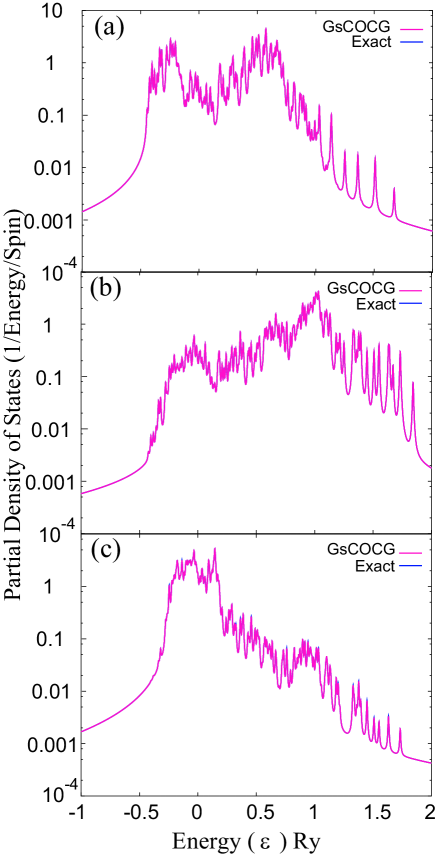
Partial densities of states are shown in Fig. 1 for a system of Au 864 atoms by NRL tight-binding Hamiltonian, tb-NRL in comparison with those by the exact calculations. In order to see the behavior of the peak positions and the tail of the peaks, the figures are drawn in the logarithmic scale. Two lines of GsCOCG and the exact calculation overlap each other almost completely and one can recognize an excellent agreement between the two different calculations.
III.3 Residual norm and convergence behavior
The useful characteristic property of GsCOCG method is the capability of monitoring the norm of residual vectors. TAKAYAMA2006 The residual vectors for the seed and shift equations with an energy (with and ) are and , respectively, and the ‘mapped’ residual vectors for the seed and shift equations and . We usually need only elements of the density matrix among near-sited orbital pairs connected by non-zero elements of the Hamiltonian or overlap matrices and the convergence monitoring is necessary for these components. TAKAYAMA2006 Therefore, in order to monitor the convergence behavior, we adopt the “residual norm” defined as
| (52) |
Furthermore, since the residual norm is different among different energy points, the average quantity (“average residual norm”) should be defined as TAKAYAMA2006
| (53) | |||||
where is the number of energy points.
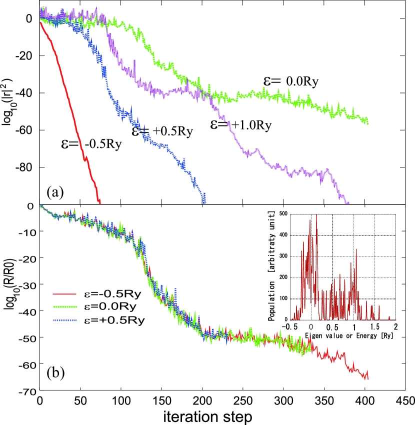
The convergence behavior of the residual norm for different seed energies is shown in Fig. 2a. The convergence at the energy of the low DOS is very fast, because the eigen-state can be constructed by a small number of basis states. The convergence of the averaged norm is shown in Fig. 2b, which confirms numerically the fact that the average residual norm (and all the physical quantities) does not depend sensitively on the choice of a seed energy.
III.4 Seed-switching technique
When one chooses a seed energy in an energy range of rapid convergence, the spectra at majority energy points have not been converged yet and one should restart the calculation with a new seed energy as seen in Fig.2a. The most desirable seed energy may be the one of the largest (partial) DOS because the convergence at these point is the most slowest.
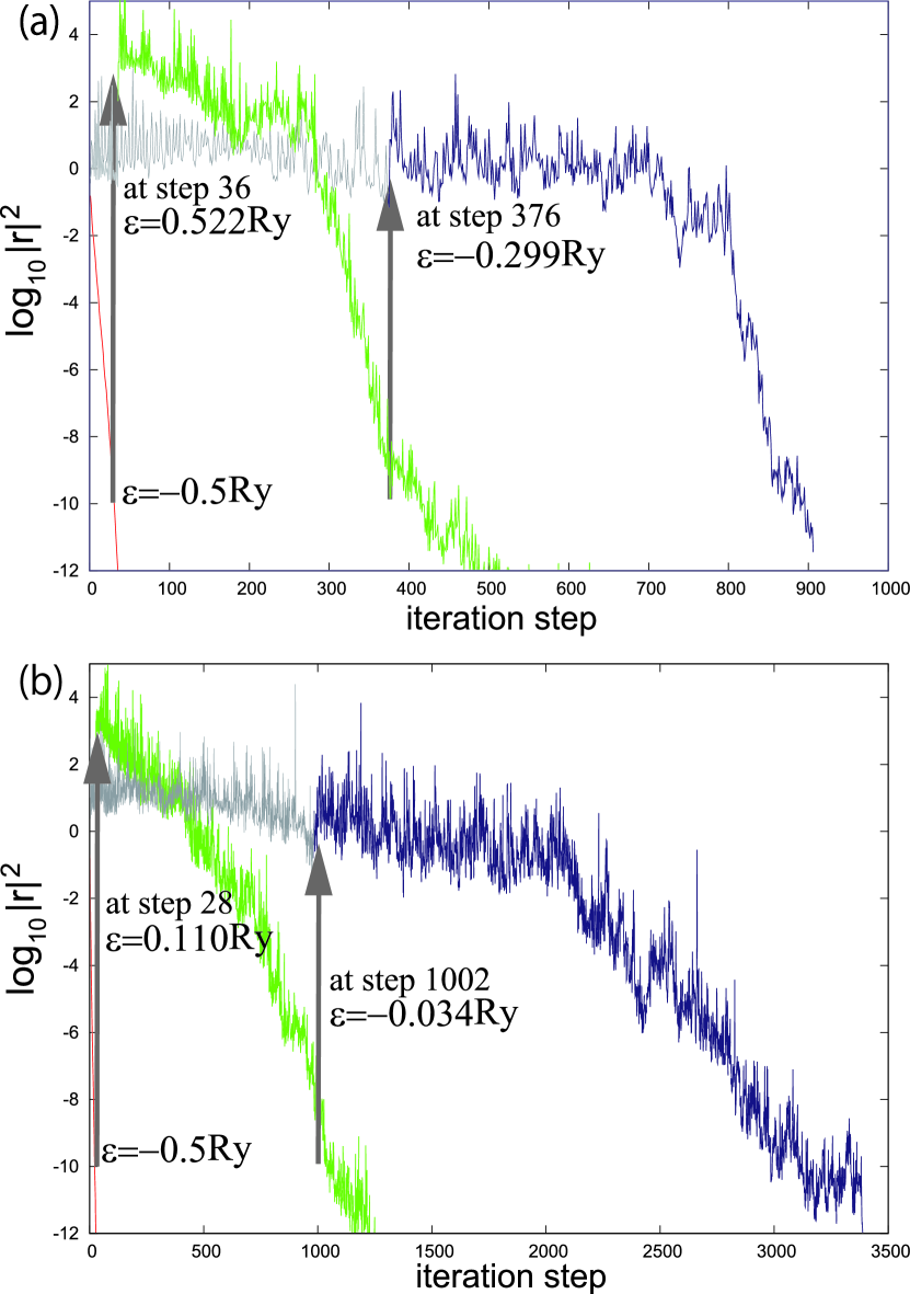
However, even if one chooses a starting seed energy in the highest DOS region and the residual norm at the seed energy reaches the convergence criterion, it often happens that there still remain several energy points/regions where the residual norm has not been small enough. Fortunately the shifting energy does not need any additional heavy computational task but several scalar manipulation as Eq.(LABEL:eq(B.32)). Because of this property of shifting energy, a choice of a seed energy can be arbitrary. As shown in Fig.2b, even if we start with an improper seed energy and switch a seed, the total iteration times for desired convergence over whole energy range is not very different. The seed-switching is very efficient technique to avoid restarting the calculation from the beginning with a new seed energy. SOGABE2007 ; yamamoto2007b One chooses a new seed energy and can continue the calculation without discarding the information of the previous calculation with the old by using the shift property. Figure 3 shows the behavior of the residual norms in the seed-switching process.
IV Generalized Lanczos process and density of states
The three-term recursive relation used in GsCOCG method leads us to the generalization of the Lanczos method. Haydock-1980 ; g-Eig-Bai ; Ozaki-Terakura-2001 As far as we know, the generalization of the Lanczos method was presented first in Ref. Haydock-1980, . In this section, we will stress that the generalized Gram-Schmidt reorthogonalization process makes G-Lanczos method practically useful and also the use of Eqs.(18) and (20) gives very efficient and accurate results.
IV.1 Generalized Lanczos process
First we define a matrix as
| (54) |
which is not self-adjoint but still satisfies the quasi-Hermitian property in the S-product;
| (55) |
We can construct the three-term procedure of the Lanczos process ( as Haydock-1980 ; g-Eig-Bai
| (56) |
where
with conditions , and then the vectors satisfy the S-orthogonality
| (57) |
This process we call the generalized Lanczos (G-Lanczos) process (method). It is well-known that the orthogonality relation is broken for larger in the Lanczos method and this is also the case here. We adopt the modified Gram-Schmidt reorthogonalization process in order to keep the -orthogonality. (See the results without the modified Gram-Schmidt reorthogonalization process in Appendix A.)
We then stop the Lanczos process up to and assume (). This procedure constructs the Krylov subspace
| (58) |
and the matrix is transformed in this subspace to a matrix of a tridiagonal form.
| G-Lanczos | GsCOCG | ||||||
| by Eq.(21) | by Eq.(22) | by Eq.(23) | by Eq.(21) | ||||
| 0.3010 8669 | 0.2926 6528 | 0.2870 0985 | 0.3006 0832 | ||||
| Eq.(21) | 5.5000 0001 | 5.4809 9705 | 5.4674 0401 | Eq.(21) | 5.5000 0000 | ||
| Eq.(22) | 5.5180 6152 | 5.4999 9998 | 5.4865 0739 | — | |||
| Eq.(23) | 5.5316 2252 | 5.5135 2184 | 5.4999 9999 | — | |||
| Eq.(26) | -0.1436 6686 | -0.1492 6754 | -0.1531 8294 | Eq.(26) | -0.1436 4084 | ||
| Eq.(27) | by Eq.(17) | -0.1311 6499 | -0.1364 7104 | -0.1403 4132 | by Eq.(38) | -0.1251 7255 | |
| by Eq.(18) | -0.1316 2401 | -0.1369 4155 | -0.1408 2023 | ||||
| Eq.(28) | by Eq.(19) | -0.1311 6490 | -0.1364 7094 | -0.1403 4123 | by Eq.(39) | -0.1436 4084 | |
| by Eq.(20) | -0.1316 2391 | -0.1369 4146 | -0.1408 2014 | ||||
Starting with a natural basis , one generates vectors in the Krylov subspace and each vector corresponds to orthonormalized linear combination of atomic orbitals (LCAO);
| (59) |
The normalized eigen-states in the generated Krylov subspace is denoted by
| (60) |
which satisfies the Schrödinger equation
| (61) |
where .
IV.2 Numerical test with NRL Hamiltonian for fcc Au
Chemical potential can be evaluated by using Eqs. (21)(23) in the generalized Lanczos method. Calculation of the Green’s function uses Eq.(13) having a double summation of atomic sites and orbitals and it consumes a long CPU time. On the contrary, the calculation of the density of states by Eq. (14) costs less CPU time. The computational efficiency will be discussed later in Section VI. Here in this subsection, we show several evaluated values, the density of states, the integrated density of states as functions of energies for a system of gold 864 atoms of fcc structure described by the tight-binding Hamiltonian constructed by Mehl and Papaconstantpolous. tb-NRL
Several evaluated values and consistency between them are summarized in Table 1. The parameters in the generalized Lanczos method are , the convergence criterion Ry in the inner CG process of . In GsCOCG, the imaginary small energy Ry, the total number of the energy integration mesh-points is 3,000, and the convergence criterion Ry in the inner CG and outer iteration procedures. The difference of the calculated total energy is of the order of Ry. The scale of the band energy is 1 Ry and the relative error may be of . The bold numbers in Table 1 are a set of consistent values in each case (for each equation determining the chemical potential) and the combination of Eqs. (17) and (19), and that of Eqs. (18) and (20) are consistent pairs of data. This consistency between the density matrix and energy density matrix is crucial for consistency between the total energy and force (Appendix B).
In GsCOCG method, calculation of Eqs. (38) and (39) needs -integration of and the numerical integration causes a certain error in the integration of the tail of the spectra. Once we reduce the value of and increase the -points of the integration, this discrepancy can be reduced. In the generalized Lanczos method, the combination of Eqs. (23), (18) and (20) is the best scheme, since we do not use the numerical energy integral.
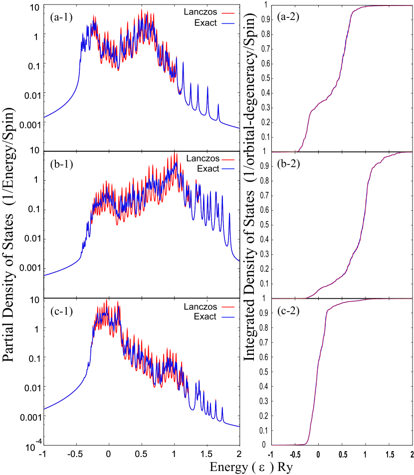
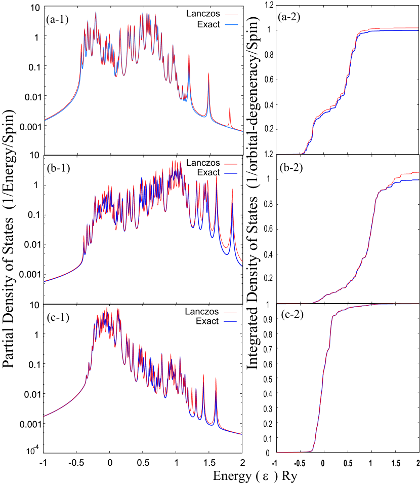
Figure 4 shows the partial density of states and integrated density of states for s-, p-, and d-orbitals. Those by the generalized Lanczos method are compared with exact results. The peak positions and the tails overlap excellently and we can conclude that the generalized Lanczos method can be powerful and convenient tool. One must notice that the exact results are more smooth in the central energy region, since the correct density of states is more dense in this energy region. In other words, the exact results reserve entire profile with peaks but, on the contrary, those by the generalized Lanczos method reserve the profiles with 51() peaks or the density of states is expressed as a polynomial function of energy of the order 51 in the present calculation.
| G-Arnoldi | GsCOCG | ||||||
| by Eq.(21) | by Eq.(22) | by Eq.(23) | by Eq.(21) | ||||
| 0.3039 0679 | 0.2928 7198 | 0.2864 6136 | 0.3006 0832 | ||||
| Eq.(21) | 5.5000 0002 | 5.4797 1790 | 5.4658 1773 | Eq.(21) | 5.5000 0000 | ||
| Eq.(22) | 5.5176 0887 | 5.5000 0001 | 5.4865 0981 | — | |||
| Eq.(23) | 5.5311 6653 | 5.5135 1949 | 5.4999 9999 | — | |||
| Eq.(26) | -0.1423 0073 | -0.1482 6563 | -0.1522 3179 | Eq.(26) | -0.1436 4084 | ||
| Eq.(27) | by Eq.(17) | -0.1300 1076 | -0.1351 4434 | -0.1389 5498 | by Eq.(38) | -0.1251 7255 | |
| by Eq.(18) | -0.1304 6635 | -0.1356 1105 | -0.1394 2996 | ||||
| Eq.(28) | by Eq.(19) | -0.1300 1076 | -0.1351 4434 | -0.1389 5498 | by Eq.(39) | -0.1436 4084 | |
| by Eq.(20) | -0.1304 6635 | -0.1356 1105 | -0.1394 2996 | ||||
V Generalized Arnoldi process and density of states
V.1 Generalized Arnoldi process
We can construct the Krylov subspace, starting with a natural basis , by using the Hamiltonian matrix , as g-Eig-Bai ; Hoshi-etal-2010
| (62) | |||||
| (63) | |||||
| (64) |
This is the Arnoldi process and we call it the generalized Arnoldi (G-Arnoldi) method. The generalized Arnoldi method generates the Krylov subspace
| (65) | |||||
The generated vector corresponds to orthonormalized LCAO
| (66) |
as in G-Lanczos method. An eigen-function satisfies the Schrödinger equation
| (67) |
where and is an upper Hessenberg matrix. We can say that this procedure is a kind of generalization of the subspace diagonalization of the Krylov subspace developed before. TAKAYAMA2004
V.2 Numerical test with NRL Hamiltonian for fcc Au
We summarize, in Table 2, several evaluated values and consistency between them, in comparison with the results of GsCOCG. The system is of 864 atoms of fcc Au by NRL tight-binding Hamiltonian. tb-NRL The bold numbers in the table are a set of consistent results in each calculation of the chemical potential. for the generalized Arnoldi process. Data of GsCOCG are the same as in Table 1. The calculated values of the total energies agree with those by the generalized Lanczos method and the overall difference is less than 1% as shown in Tables 1.
Figure 5 shows the partial density of states and the integrated density of states as functions of energies. The peak positions are deviated slightly from those by the exact calculation, which one could make smaller with increasing a dimension of the Krylov subspace.
VI Comparison among GsCOCG, G-Lanczos method and G-Arnoldi method
VI.1 Convergence
The dimension of the Krylov subspace in GsCOCG, G-Lanczos or G-Arnoldi methods equals to where is the maximum iteration step. GsCOCG method is very accurate method if one achieves the iteration to have enough small residual norm (e.g. Ry). In Fig.2, we have shown the convergence behavior of the residual norms with different seed energies and until much smaller convergence region. One should use the same iteration criteria both in the inner CG and outer procedures in GsCOCG method. It sometimes happens that the resultant DOS shows an un-physical behavior, e.g. negative values of DOS, if one stops the iteration steps before enough convergence in GsCOCG method. On the other hand, G-Lanczos and G-Arnoldi methods never give such un-physical DOS even if one stops at small iteration step because of the expression of Eq.(13). Furthermore, the first moments are preserved correctly in the energy spectra of G-Lanczos method. In the spectrum of the present model by the exact calculation, we observe about forty prominent peaks and then we use in the calculations of G-Lanczos and G-Arnoldi procedures. This is presumably the reason why the peak positions and detailed profiles in the spectra of G-Lanczos method show excellent agreement with those of the exact calculation. G-Lanczos method needs the Gram-Schmidt reorthogonalization and also it is necessary to have enough convergence in the inner CG procedure. G-Arnoldi method does not need such reorthogonalization procedure since one solve the eigen-value problem in that subspace.
In condensed matters, the width of the valence and/or conduction bands may be of the order of 1Ry. Then, when the number of atoms is , we can estimate the separation of each energy level as of the order of . Presumably 10% of this separation would be an enough accuracy in the energy scale. In our present case, with , the convergence criterion can be chosen as Ry. We also observed that the maximum iteration steps are almost the same for the convergence criterion and in GsCOCG and G-Lanczos methods. This is the reason why we choose Ry.
| G-Lanczos | (864 atoms) | (256 atoms) | ||
|---|---|---|---|---|
| Eq.(22) | 0.2926 6528 | 0.2875 4133 | ||
| Eq.(27) | -0.1364 7104 | -0.1358 7639 | ||
| G-Arnoldi | (864 atoms) | (256 atoms) | ||
| Eq.(22) | 0.2928 7198 | 0.2886 2149 | ||
| Eq.(27) | -0.1351 4434 | -0.1346 6195 | ||
| GsCOCG | (864 atoms) | (256 atoms) | ||
| Eq.(21) | 0.3006 0832 | 0.2947 1535 | ||
| Eq.(26) | -0.1436 4084 | -0.1433 1925 |
We compare the results of the chemical potential and the total band energy of systems of 256 and 864 atoms in Table 3. The difference of the chemical potential is of the order of Ry, and that of the total band energy is of the order of Ry. The level separation in 256 atom system can be estimated as Ry and that in 864 atom system Ry. The difference in the chemical potential of two systems of different sizes is due to the difference of total number of levels which changes the value of the chemical potential sensitively. On the other hand, the difference of is just the quantity related to the overall spectrum and we can see an excellent convergence of the results of .
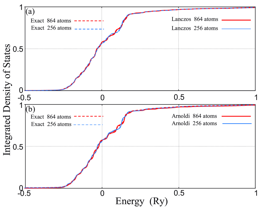
Figure 6 shows the actual convergence behavior of IDOS by G-Lanczos and G-Arnoldi method. The agreement between the results by G-Lanczos or G-Arnoldi methods and those by the exact calculation is excellent both for systems of 864 atoms and that of 256 if we adopt . The most apparent difference appears in the IDOS curves of exact calculation of systems of 256 atoms and 865 atoms in the mid energy region, and the calculated results by our present methods present this difference with complete fidelity.
| (a) Au 256 | CPU-times (s) | ||
|---|---|---|---|
| G-Arnoldi | main part | 0.52 1.11 | — |
| total | 1.59 3.20 | — | |
| G-Lanczos | inner CG | 2.04 3.89 | — |
| main part | 2.89 5.60 | — | |
| total | 3.92 7.62 | — | |
| GsCOCG | seed | — | 13.67 |
| shifted | — | 7.53 | |
| total | — | 21.20 | |
| Exact | — | 57.60 | |
| (b) Au 864 | CPU-times (s) | ||
| G-Arnoldi | main part | 1.94 3.76 | — |
| total | 3.00 6.00 | — | |
| G-Lanczos | inner CG | 7.93 15.13 | — |
| main part | 10.87 21.13 | — | |
| total | 11.93 23.31 | — | |
| GsCOCG | seed | — | 140.89 |
| shifted | — | 108.36 | |
| total | — | 249.15 | |
| Exact | — | 2111.51 |
VI.2 CPU times
We summarize, in Tables 4, the CPU times (by using single CPU of the standard workstation) for (s-orbitals) of the generalized Lanczos and the generalized Arnoldi methods with Eq.(14), that of GsCOCG with Eq.(37), and that of the exact diagonalization method for the NRL Hamiltonian of fcc Au system of 256 and 864 atoms. tb-NRL The total number of orbitals equals to nine times of the total number of atoms (1 s, 3 p’s and 5 d’s). We use, in the inner CG process of the generalized Lanczos (G-Lanczos) method, the convergence criterion Ry. Two numbers in the row of the CPU time are referred to those of and , respectively, for G-Lanczos and G-Arnoldi methods, though the results of almost coincide with those of . For GsCOCG (with shifted 3,000 energy points), the data shown here are those of Ry both for in the inner and outer iteration processes. The repeated time of the inner CG process ( part) in GsCOCG and G-Lanczos method is . (Repeated time of is needed for Ry.)
The system size dependence of the CPU time is linear for the generalized Arnoldi (G-Arnoldi) method and the generalized Lanczos (G-Lanczos) method, bilinear for GsCOCG method and cubic for the exact calculation. The generalized Arnoldi method is extremely efficient in electronic structure calculations of extra-large systems with several hundred thousands atoms.
VI.3 Applicability to large-scale electronic structure calculations and MD simulations
In the exact calculation and GsCOCG method, calculations of physical properties, such as the density matrix, the energy density matrix, and chemical potential, require the numerical integration as in Eqs. (21), (26), (38) and (39). Therefore, in order to keep high accuracy, the integration needs fine energy mesh points. On the other hand, the generalized Lanczos or the generalized Arnoldi methods use the simple summation of the eigen-states in the mapped subspace in Eqs. (22), (23), and (17) (20). These two methods do not consume the CPU time and give stable values of the density matrix and the energy density matrix.
The CPU times per one MD-step are, for the present models, a few seconds by the generalized Lanczos method and the generalized Arnoldi method. From the above comparison among various viewpoints, we can conclude that the generalized Lanczos method or the generalized Arnoldi method are very suitable to large-scale electronic structure calculations and MD simulation of several tens of thousands atoms and a long MD-steps. On the other hand, GsCOCG method can give excellently rigorous results with more CPU times and may be applicable to problems of a fixed atomic configuration (but not for the MD simulation).
GsCOCG method is based on the three-term recursive equations and we need store three generated vectors at each recursive process. Of course, when the size of the Hamiltonian and overlap matrices are extremely large and the memory size becomes a serious obstacle, (though much smaller consumption than the exact diagonalization method, ) we should invent other method of much faster convergence and smaller cost of memory size.
The convergence criterion might corresponds to the range of neighboring 1,000 atoms, as already discussed, and we do not observe any clear difference between results by the present methods and the exact calculations. Even when we should discuss some physics of nano-scale systems, the electronic structure is determined by some nearby surroundings. This idea we call near-sitedness. Kohn1996 Even when we have to deal with a much larger systems, we can use smaller interaction range than the system size due to the near-sitedness. Presumably more serious problem of the system size in some specific problems, for examples, entire calculation of nano-devise or the electron-strain field interaction such as fracture propagation Si-fracture-1 ; Si-fracture-2 and dislocation. Miyata2001
VII Conclusion
We have derived several efficient and accurate algebraic methods to calculate the Green’s functions, total/partial density of states and total band energy in case of non-orthogonal atomic orbitals. The method is very general.
We have investigated the accuracy and efficiency by showing numerical data with different numerical procedures. GsCOCG is very accurate with less consumption than the exact diagonalization but may not be appropriate for long MD-step simulations. The generalized Lanczos method becomes applicable to actual large systems with the modified Gram-Schmidt reorthogonalization to maintain the orthogonality of generated basis vectors. Then, the generalized Arnoldi method and the generalized Lanczos method are accurate and efficient, and their CPU times depend linearly upon the system size. Therefore, these two methods would be the most suitable to the large-scale electronic structure calculations and MD simulations. A crucial point we should point out finally is the fact that G-Lanczos and G-Arnoldi methods do not adopt any numerical integration in energy which leads additional numerical error.
Acknowledgments
One of authors (T. Fujiwara) expresses sincere thanks to TOYOTA Motor Corporation for the financial support. Numerical calculation was partly carried out using the supercomputer facilities of the Institute for Solid State Physics, University of Tokyo. Our research progress of large-scale systems and other information can be found on the WEB page of ELSES (Extra-Large Scale Electronic Structure calculation) Consortium; http://www.elses.jp.
Appendix A Re-orthogonalization by modified Gram-Schmidt method
The three-term recursive relation in the generalized Lanczos method guarantees theoretically the automatic S-orthogonalization. However, the orthogonality is broken in the numerical calculation procedure. This problem causes several troubles such as the existence of constant background of error in the spectrum, TAKAYAMA2006 appearance of “ghost” structure in spectrum due to erroneous mixing of states and a broken normalization of the partial density of states.
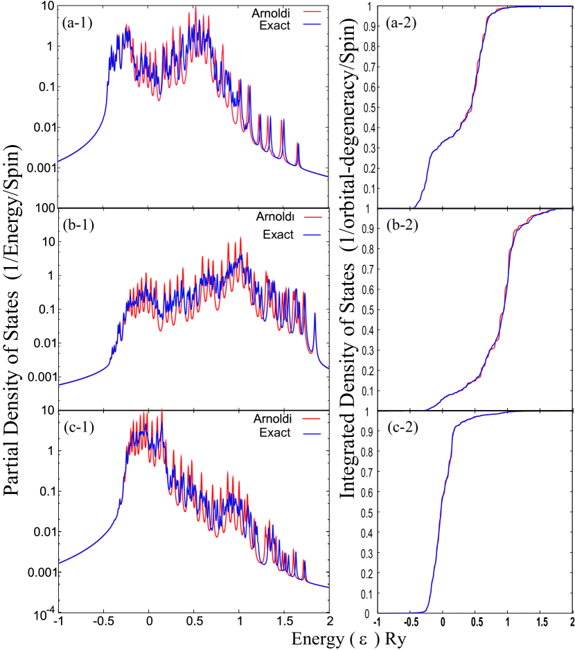
Figure 7 shows the examples of this broken orthonormality, in a system of 256 atoms of fcc Au by using the NRL Hamiltonian. One can see the “ghost” peaks (e.g. at Ry in (a-1), at Ry in (b-1) and (c-1)) and broken normalization (e.g. in (a-2) and (b-2)). These problems are solved by the re-orthogonalization with the modified Gram-Schmidt method.
Appendix B Consistency between the total energy minimum and a vanishing force
We should construct our eigen-states in a small subspace and a certain numerical error is unavoidable in evaluated total energy and force. Even in that case, the consistency between the total band energy minimization and an vanishing atomic force is the most important in the electronic structure calculation in equilibrium atom configuration. In the framework of the tight-binding model, the force (due to band energy) acting on an atom is evaluated by a formula
| (68) |
which can be rewritten, with only an assumption of the eigen-state property Eq.(8) in the mapped subspace, as
| (69) | |||||
Therefore, calculated atomic and electronic configuration of the minimum total energy is consistent with that of vanishing atomic force, if the identity is satisfied always in any atomic configuration. It should be noticed that the above equality is satisfied in the mapped subspace as described in II.3.2. It is important in actual calculating procedure that we should use the consistent pair of equations as Eqs. (17) and (19) or Eqs. (18) and (20).
References
- (1) T. Hoshi and T. Fujiwara, J. Phys. Soc. Jpn. 72, 2429 (2003).
- (2) T. Hoshi, Y. Iguchi and T. Fujiwara, Phys. Rev. B 72, 075323 (2005).
- (3) Y. Iguchi, T. Hoshi and T. Fujiwara, Phys. Rev. Lett. 99, 125507 (2007).
- (4) T. Hoshi and T. Fujiwara, J. Phys. Condensed Matters 21, 272201 (2009).
- (5) S. Goedecker, Rev. Mod. Phys. 71, 1085 (1999)
- (6) S. Goedecker and L. Colombo, Phys. Rev. Lett. 73, 122 (1994).
- (7) W. Yang, Phys. Rev. Lett. 66, 1438 (1991); T. Ozaki, Phys. Rev. B74, 245101 (2006).
- (8) X.-P. Li, R. W. Nunes, and D. Vanderbilt, Phys. Rev. B 47, 10891 (1993).
- (9) F. Mauri, G. Galli, and R. Car, Phys. Rev. B 47, 9973 (1993).
- (10) C.-K. Skylaris, P. D. Haynes, A. A. Mostofi, and M. C. Payne, J. Chem. Phys. 122, 084119 (2005).
- (11) J. M. Soler1, E. Artacho, J. D Gale, A. García, J. Junquera1, P. Ordejón, and D. Sánchez-Portal, J. Phys. Condens. Matter 14, 2745 (2002).
- (12) P. Ordejón, Comp. Mat. Sci. 12, 157 (1998).
- (13) R. Takayama, T. Hoshi and T. Fujiwara, J. Phys. Soc. Jpn. 73, 1519 (2004).
- (14) R. Takayama, T. Hoshi, T. Sogabe, S-L. Zhang and T. Fujiwara, Phys. Rev. B 73, 165108 (2006).
- (15) T. Sogabe, T. Hoshi, S.-L. Zhang, and T. Fujiwara, Electronic Transactions on Numerical Analysis (ETNA), 31, 126 (2008).
- (16) T. Sogabe, T. Hoshi, S.-L. Zhang, and T. Fujiwara, Frontiers of Computational Science, pp. 189-195, Ed. Y. Kaneda, H. Kawamura and M. Sasai, (Springer Verlag, Berlin Heidelberg, 2007).
- (17) C. Lanczos, J. Res. Natl Bur. Stand. 45, 225 (1950); C. Lanczos, J. Res. Natl Bur. Stand. 49 33 (1952).
- (18) R. Haydock, Solid State Physics 35 pp.225-228, Ed. H. Ehrenreich, F. Seitz, and D. Turnbull (Academic Press, New York,1980).
- (19) Templates for the Solution of Algebraic Eigenvalue Problems, Chapter 5, Edited by Z. Bai, J. Demmel, J. Dongrarra, A. Ruhe, and H. van der Vorst, (SIAM, Philadelphia, 2000).
- (20) M. Elstner, D. Porezag, G. Jungnickel, J. Elsner, M. Haugk, Th. Frauenheim, S. Suhai and G. Seifert, Phys. Rev. B 58, 7260 (1998).
- (21) T. Fujiwara, T. Hoshi, and S. Yamamoto, J. Phys.: Condens. Matter 20, 294202 (2008).
- (22) T. Sogabe and S.-L. Zhang, talk in the International Conference Numerical Analysis and Scientific Computing with Applications, Agadir, Morocco, May 18-22, 2009; in preparation, T. Sogabe, T. Hoshi, S.-L. Zhang and T. Fujiwara, Solution of Generalized Shifted Linear Systems with Complex Symmetric Matrices.
- (23) A. Frommer, Computing 70, 87 (2003).
- (24) M. J. Mehl and D. A. Papaconstantopoulos, Phys. Rev. B 54, 4519 (1996); F. Kirchhoff, M. J. Mehl, N. I. Papanicolaou, D. A. Papaconstantopoulos, and F. S. Khan, Phys. Rev. B 63, 195101 (2001).
- (25) S. Yamamoto, T. Sogabe, T. Hoshi, S.-L. Zhang, and T. Fujiwara, J. Phys. Soc. Jpn 77, 114713 (2008).
- (26) T. Ozaki and K. Terakura, Phys. Rev. B 64, 195126 (2001).
- (27) T. Hoshi, T. Fujiwara, S. Nishino, S. Yamamoto, Y. Zempo, M.Ishida, T. Sogabe, and S.-L. Zhang, in preparation.
- (28) W.Kohn, Phys. Rev. Lett. 76, 3168 (1996).
- (29) M. Miyata and T. Fujiwara, Phys. Rev. B 63, 045206 (2001).