Dynamic Phase Transition from Localized to Spatiotemporal Chaos in Coupled Circle Map with Feedback.

Abstract

We investigate coupled circle maps in presence of feedback and explore various dynamical phases observed in this system of coupled high dimensional maps. We observe an interesting transition from localized chaos to spatiotemporal chaos. We study this transition as a dynamic phase transition. We observe that persistence acts as an excellent quantifier to describe this transition. Taking the location of the fixed point of circle map (which does not change with feedback) as a reference point, we compute number of sites which have been greater than (less than) the fixed point till time $t$. Though local dynamics is high-dimensional in this case, this definition of persistence which tracks a single variable is an excellent quantifier for this transition. In most cases, we also obtain a well defined persistence exponent at the critical point and observe conventional scaling as seen in second order phase transitions. This indicates that persistence could work as good order parameter for transitions from fully or partially arrested phase. We also give an explanation of gaps in eigenvalue spectrum of the Jacobian of localized state.

Coupled map lattices have been investigated extensively in past few decades. The dynamics can show very novel features when local dynamics is higher dimensional. Using feedback to make the local dynamics higher dimensional makes it possible to systematically increase dimensionality of local map without changing several other features such as location of fixed point. Investigation of phase diagram of such a system shows possibility of existence of partially arrested state in which certain sites are near the fixed point while others are not. We study the nonequilibrium phase transition from such a state to a state of spatiotemporal chaos and propose that persistence works as an excellent order parameter for such transitions.

I Introduction

Pattern formation in spatially extended systems has been an object of extensive study in past few decades. The reasons for the interest in pattern formation are not far to seek. Pattern formation happens in several natural systems and scientists are interested in understanding it. Examples could be flame propagation or occurrence of spirals in a chemical reactions or patterns on the skins of animals modeled by reaction-diffusion processes. Several systems like biological patterns biology (1991), charge density waves or Josephson Junction Arrays JJA (1988); bak ; Joseph (1996), lasers rroy (2007) have been studied extensively from the viewpoint of dynamics and pattern formation. The practical importance of understanding above systems can not be overemphasized. Partial differential equations, coupled ordinary differential equations, coupled oscillator arrays and coupled maps have all been used to model different physical and biological systems and have uncovered interesting modifications of equilibrium, bifurcations and stability properties of collective spatiotemporal states. These systems have been studied extensivelycross (1993); footnote1 . However, while we have arrived at a good understanding of low dimensional chaos in past two decades, and understood routes to chaos in several seemingly disparate systems in an unified manner, the same is not true for spatiotemporal systems.

As one would expect, there is practical relevance to these models. Certain simplified models of spatiotemporal dynamics have been studied extensively in recent past. We would like to make a special mention of coupled map lattices which have been studied extensively in the hope that the understanding we have developed in low-dimensional systems could be useful in understanding spatiotemporal dynamics. Majority of the studies are in coupled one-dimensional maps. At times, they have been successful in modeling certain patterns observed in spatiotemporal systems. For example, the phenomena of spatiotemporal intermittency in Rayleigh-Benard convection has been modeled by coupled map lattices chate (1988); bigazzi (1988). They have been used to model spiral waves in B-Z reaction barkley (1990) and even in crystal growth reynolds (1990).

We feel that these studies could be helped considerably by quantitatively identifying different phases in the system and attempting to understand transitions between those. A lot of attention has been devoted to transition to synchronization in these systems which is easy to identify and analyze. However, other spatiotemporal patterns are far less analyzed and understood.

It is worth noting that in several spatiotemporal systems the field is high dimensional. For example, for a chemical reaction, we would require information about concentrations of all reactants and products at all points to be able to simulate the system. There are several phenomena which are possible only when dynamics is higher dimensional. On the other hand most of the existing studies in coupled map lattices are about coupled one-dimensional maps and very few involving high dimensional maps, for example coupled Chialvo’s map jampa (2007), coupled Henon map politi_chaos92 (1992), Arnold’s cat map bonetto_CUP (2005), modified Baker’s map for Ising model sakaguchi_pre99 (1999), etc. Here we try to study coupled higher dimensional maps. We try to systematically change the dimensionality of the map and study coupled maps with feedback where the feedback time could be varied.

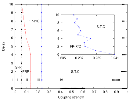
Figure 1: We plot the phase diagram of coupled circle map with delay in two parameter space of coupling strength $\epsilon$ and delay time $\tau$. The abbreviation SFP, FRP, FP-P/C and STC denote Synchronous fixed point, Frozen random pattern, Fixed point-Periodic/Chaotic cycles and Spatiotemporal chaos respectively. In the inset, we magnify the phase boundary between FP-P/C regime and STC regime. We can have only integer values of feedback time and the lines in phase diagram are guide to the eye. The black solid circles indicate points in phase space where spatiotemporal fixed point phase is seen.

In coupled map lattice (CML) kaneko (1993) time evolution is conflict between competing tendencies: the diffusive coupling between units tends to make the system homogeneous in space, while the chaotic map produces temporal inhomogeneity, due to sensitive dependence on initial condition. Such systems display a rich phase diagram and origin and stability of various phases in these systems are of theoretical and practical interest. The transitions between various phases in these systems could be viewed as dynamic phase transitions. Though these are clearly non-equilibrium systems, different techniques used in the study of equilibrium phase transitions have been applied to explore the variety of phenomenologically distinct behaviors. Such non-equilibrium systems range from growths of surfacesstanley (1995) to traffic jams in vehicular traffic and granular flowswolf (1996); haye (2000). For such analysis, there is a need to define an order parameter that will characterize the transition. However, not many dynamic phase transitions have been studied from this viewpoint gupte72 (2005); gupte74 (2006); rahulpandit (2000); gade (2007); ashwini (2010). Most of the studies are devoted to transition in models with so-called absorbing states. In the context of synchronization, there have been extensive studies to ascertain whether or not this transition is in the universality class of directed percolation ginelli (2003). Transition to synchronization, locking in of the dynamics of several systems to a collective oscillation, is an important but minuscule part of overall spatially extended systems. Several non-synchronization transitions have been observed such as spiral state to spatiotemporal chaos rahulpandit (2000), traveling wave to spatiotemporal chaos gade (2007). The spatiotemporal dynamics is far richer and other transitions deserve attention.

As suggested by Pyragas, feedback in the dynamical systems can play a central role in controlling chaos by stabilizing UPO’s embedded in chaotic attractorPyragas (1992). The scheme has been efficiently implemented in wide range of experimental applications. Feedback leading to synchronization is a well established fact supported by several researchershandbook (1993). Though feedback has been an important aspect of studies in control and synchronization, not much has been said about its effect on different dynamical phases. It is then important to find the effects of feedback in terms of alterations in system dynamics that may lead to origin of different dynamic phases.

In this work, we investigate coupled maps with feedback. As mentioned before, coupled higher dimensional maps have not been studied adequately. Using feedback, we can systematically vary dimensionality of local map using feedback and study its effect on overall dynamics. We note that the feedback as defined in our model does not change the location of fixed point of system without feedback. We have used it extensively as a reference point. This allows us to study spatially extended higher dimensional systems with known properties. We investigate a model of coupled circle maps with feedback. The strength of feedback and the delay time are the parameters in the system. We will present a general phase diagram of the system. In particular, we observe a novel transition from localized chaos to spatiotemporal chaos. By localized chaos, we mean that the laminar and turbulent phases coexist in the same space domain for weaker couplings. The reason to call it localized chaos is that one can see there are well defined boundaries of turbulent sites which do not mix with laminar ones. A similar pattern has been named spatial intermittency (SI) in previous studies and some of its properties such as eigenvalue spectrum of Jacobian are found to be related to its dynamical propertiesgupte72 (2005); gupte74 (2006). Interestingly, we find that persistence acts in effective way to characterize and quantify certain dynamical phases and transition between them in this system. Thus, persistence can be taken as excellent order parameter for certain phase transitions.

The plan of paper is as follows. We introduce the model in the section II. In Section III, we make a detailed analysis of one of the phases, namely localized chaos and calculate quantities such as turbulent length distribution. In section IV, we present our investigations in transition between localized chaos regime and spatiotemporal chaos and we present evidence that persistence acts as an excellent order parameter to characterize the transition. In section V, we demonstrate that some characteristic features in eigenvalue distributions of Jacobian can distinguish between different dynamical phases.

II Model

We define model of coupled circle maps with feedback as follows. We assign a continuous variable $x_{i}(t)$ at each site $i$ at time $t$ where $1\leq\;i\leq N$. $N$ is the number of lattice points. The evolution of $x_{i}(t)$ is defined by,

$$x_{i}(t+1)=(1-\epsilon-\delta)f(x_{i}(t))\;+\;{\frac{\epsilon}{2}}\;[f(x_{i-1}(t))$$

$$+f(x_{i+1}(t))]+\delta f(x_{i}(t-\tau))$$ (1)

The parameter $\epsilon$ is the coupling strength and the local dynamical update function $f(x)$ is the sine-circle map,

$$f(x)=x+\omega-{\frac{k}{2\pi}}\;\sin(2\pi x)$$ (2)

Where, $k$ is the strength of nonlinearity and $\omega$ is the winding number. The parameter $\delta$ is strength of feedback and $\tau$ is delay time. If we increase $\tau$, we can increase the dimension of map. In our simulations, we confine values of parameters to $\delta=0.1$, $k=1$ and $\omega=0.068$. The coupling topology considered here is diffusive i.e nearest - neighbor connections. For coupled circle map, we confine the dynamics in the interval $[0,1]$ using the following rule. If int$[x_{i}(t)]=m$, $x_{i}(t)=x_{i}(t)-m$ if $x_{i}(t)>0$ and $x_{i}(t)=x_{i}(t)-m+1$ if $x_{i}(t)<0$. We study the system with random initial conditions. The system is updated synchronously with periodic boundary condition. The feedback does not change the fixed point solution of local map $f(x)$ without feedback. The fixed point solution for the local map $f(x)$ is given by, $x^{*}={\frac{1}{2\pi}}\sin^{-1}({\frac{2\pi\omega}{k}})$. The parameter values considered here yield the value of fixed point as $x^{*}=0.07026$. This point acts as an excellent reference point in visualizing the dynamical behavior of system and also in symbolic dynamics of the system. We can define the site dynamics to be laminar if $|x_{i}(t)-x^{*}|<\eta$ for small enough neighborhood $\eta=0.001$ and to be turbulent otherwise.

III Spatiotemporal Dynamics

We examine the phenomenology of delay coupled circle map with feedback under variation of coupling strengths and delay time. Various spatiotemporal patterns are clearly evident from phase diagram Fig. 1 and the bifurcation diagram shown in Fig. 2. Note that on y axis of Fig. 1, the time is discrete. The delay time $\tau$ can only be some integer. The phase boundary of various regions can be seen.

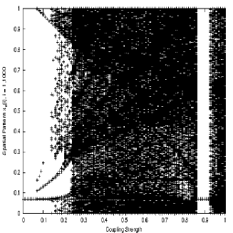
Figure 2: Bifurcation diagram of Spatial pattern at an instant of time (after transience), with respect to coupling strength $\epsilon$ for delay time $\tau=1$.

Increasing value of $\tau$ is equivalent to increasing the dimensionality of local dynamics. There are clearly four distinct behaviors shown by the system as seen from phase diagram Fig. 1. The first region in phase diagram labeled as SFP (Synchronous fixed point) where, for smaller coupling strengths $\epsilon\leq 0.06$ the entire system goes to local fixed point $x^{*}$. This is an absorbing state and system settles in this state very quickly. We have checked that this state exists at least for $\tau\leq 10$. For higher coupling strengths, The system goes to spatiotemporal chaos as shown in phase diagram marked as STC. These different behaviors can also be visualized using the bifurcation diagram Fig. 2 obtained for different coupling strengths for $\tau=1$. This bifurcation diagram shows the state of all sites at a given instant of time. For very high coupling strengths, the system shows some stability islands for some values of $\tau$ though they constitute a small part in phase diagram, we find them worth a mention.

In the intermediate coupling strengths, the system shows a rather interesting behavior. We can see that some of the sites approach local fixed point and some of the sites take on different values which do not change in time. This behavior is shown in phase diagram marked as FRP which stand for frozen random pattern frozen (1993). This region is characterized by a spatial sequence of different domains whose size and periodicity may greatly vary. Upon further increase of coupling strengths, one enters in a region where we can see coexistence of different dynamical regimes. Where some of the sites indeed go to fixed point, some of the sites show periodic/chaotic behavior. This is an interesting state where one can see that different dynamical phases do not mix with each other. The regions marked as FRP and FP-P/C in the phase diagram collectively represent the dynamics which we refer to as Localized chaos. Chaos is localized in certain dynamical regimes of turbulence and does not interfere with evolution of laminar states. In localized chaos regime, chaotic domains and periodic domains are fixed in space. This is evident from spatial distribution pattern. The perturbations do not propagate in space. Essentially, the dynamics is non-spreading and non-infective in nature, i.e. the spatially intermittent solutions have zero velocity components in spatial direction, and modes traveling along the lattice are absent. This can also be considered as a case of spatial intermittency gupte72 (2005). The important result is that spatial intermittency is seen over a large parameter regime in presence of feedback. For each feedback time, we have a well defined region where we get the transition. These spatiotemporal patterns are clearly evident from space-time density plots below. Each figure represent a particular region in phase diagram.

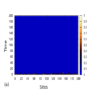
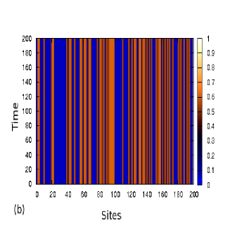
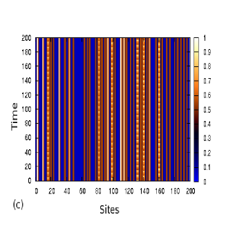
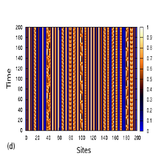
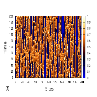
Figure 3: (Color online)Space time density plot of coupled circle map lattice with feedback defined through eqs. (1)-(2), in a system of size $L=200$, for parameters $k=1$, $\delta=0.1$, $\omega=0.068$ for $\tau=1$ and (a)$\epsilon=0.05$, (b) $\epsilon=0.1$, (c)$\epsilon=0.16$, (d) $\epsilon=0.23$,(e) $\epsilon=0.24097$, and (f) $\epsilon=0.245$

Fig. 3 shows space-time density plots of $x_{i,t}$ for six choices of parameter values. The site index is plotted along the x-axis and the time evolves along the y-axis. As mentioned previously, laminar regions are blue (dark grey) in this representation. The colorbar shows different value of $x(i)$ according to given scale. Fig. 3(a) gives the space-time density plot for parameter values where the system goes to spatiotemporal fixed point. Fig. 3(b) shows the plot for non infective and non spreading behavior called as frozen random pattern. Fig. 3(c) and (d) shows coexistence of different dynamical regimes for which the dynamics essentially remains ‘arrested’. Fig.3(e) shows density plot for $\epsilon=0.24097$ which is critical point for the transition, we can see the spreading behavior just emerging in the system. Fig.3(f) depicts fully grown spatiotemporal chaos and here we can see that the state variable encompasses much larger part of available phase space.

Figure 4: (a) The distribution of turbulent phase lengths for coupling values $\epsilon=0.14,0.16,0.23,0.245$ for $\tau=1$. The fit to this distribution is exponential with exponent $\beta$. The ordinate axis is presented in logarithmic scale. (b) This plot shows exponent $\beta$ vs coupling strength $\epsilon$ for $\tau=1$.

The number of turbulent sites increase as coupling strength increases. Note here that, all those sites which are not laminar are considered turbulent. We calculate distribution of turbulent phase length. It is observed that turbulent length distribution is governed by the exponential law,

$$T(l)=A\exp(-\beta l)$$ (3)

where, exponent $\beta$ is the rate of decay and $l$ is the the cluster size of turbulent sites. Fig. 4(a) shows Cumulative distribution of turbulent lengths for coupling parameter values $\epsilon=0.1,0.16,0.23,0.245$. We can see that the distribution for smaller coupling strengths falls of quickly as opposed to higher value of coupling strength where the exponential decay is slower indicating large number of turbulent phases. Fig. 4(b) shows how the exponent $\beta$ varies with respect to $\epsilon$. There is a sharp increase in value of beta near $\epsilon\sim 0.24$ .

IV Persistence as an Order Parameter

As it can be seen the system displays a dynamical phase transition i.e. from localized chaos regime to spatiotemporal chaos. It is important to find a good quantifier to quantify this transition. This is a partially arrested state and in partially or fully arrested dynamical states, we believe that persistence acts as a good order parameter. There have been couple of previous studied in persistence in coupled map lattices by Menon et al. and by Gade et al.. Menon et al. found that it was a good indicator for a transition from fully synchronous state to spatiotemporal chaos while Gade et al. found that its dynamical behavior is able to characterize even traveling wave state which can be seen as a partially arrested state in moving frame of referencemenon (2003); gade (2007). It was observed by us in preliminary version of these studies abhijeet_dae (2006) that persistence acts as an good quantifier. Recent results by Mahajan and Gade show that local persistence can also characterize the transition from clustered state to spatiotemporal chaos in small world networksashwini (2010). This definition of persistence concentrates on a single variable and one would wonders if it is adequate for the high dimensional local dynamics we are studying in this case. However, we find that persistence acts as an excellent order parameter for distinguishing between partially and fully arrested states in this system. This demonstrates a generic utility of persistence as order parameter even in transitions from partially arrested phase. Thus, it is possible that persistence is a good characteristic for systems in which dynamics is partially or fully localized. Conventionally, persistence in the context of stochastic processes has been defined as the probability $P(t)$ that a stochastically fluctuating variable with a zero mean has not crossed a threshold value up to time $t$ satya (1999). For a spin system with discrete states, such as Ising or Potts spins, it is defined in terms of the probability that a given spin has not flipped out of its initial state up to time $t$. The power-law tail of $P(t)$, i.e.

$$P(t)\sim 1/t^{\theta},$$ (4)

defines the persistence exponent $\theta$. The exponent $\theta$ is dimension-dependent, non-trivial exponent. For spatially-extended systems, the time evolution of the stochastic field at one lattice site is coupled to its neighbors. This makes the effective single-site evolution essentially non-markovian and renders the nontriviality to the exponent $\theta$. This nature of local persistence probability relates it to infinite point correlation function in time direction koduvely (1998).

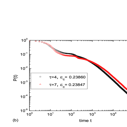
Figure 5: (a) Persistence probability $P(t)$ is plotted as a function of time $t$ on a logarithmic scale for $k=1$, $\omega=0.068$ and $\tau=1$. The lattice size is 5000. The curves shown are for $\epsilon=0.24040$ (upper), $\epsilon=0.24097$ (middle), and $\epsilon=0.24300$ (lower). The line with slop 1.31 is plotted for reference. (b) (Color online) Log P(t) vs Log t for $\tau=4$, $\tau=7$.

A natural generalization of the idea to CML as suggested by Menon et al. menon (2003), defines local persistence in terms of the probability that a local state variable $x_{(i,t)}$ does not cross fixed point value $x^{*}$ up to time $t$. With this definition, we study persistence in the coupled map lattice defined through eq (1), via simulations on systems with various lattice sizes. The persistence defined above is referred as local persistence in literature. In this work, we study only local persistence and do not study any other definition of persistence. In this paper, by persistence we mean local persistence only. We start with local $x_{i}$ distributed randomly over interval $[0,1]$. We find the normalized fraction of persistent sites, defined as sites for which $x_{i,t}$ has not crossed $x^{*}$ up to time $t$. Thus, sites for which the sign of $(x_{i,t}-x^{*})$ has not changed unto time $t$ are persistent at time $t$. This persistence probability $P(t)$ is averaged over an ensemble of over 2000 random initial conditions.

Fig. 5(a) shows plots of P(t) at three different values of coupling parameter $\epsilon$. It can be easily noted that for values below critical point $P(t)$ saturates. For the value above critical point i.e. in chaotic domain, $P(t)$ decays exponentially. Exactly at the critical point of transition between localized chaos to spatiotemporal chaotic regimes, $P(t)$ decays as a power law, which defines the persistence exponent $\theta=1.31$. The power law decay can also be seen for other values of $\tau$ footnote2 . Fig. 5(b) shows persistence distribution for $\tau=4,7$ at the critical points $\epsilon_{c}=0.2386$ and $\epsilon_{c}=0.23847$ respectively. The observed power-law behavior in 1+1 dimension suggests the further investigation of parameters involved in phenomenological scaling laws. The distance from criticality $\Delta=|\epsilon-\epsilon_{c}|$ and lateral system size $L$ can be used as parameters to study scaling properties of the system. One would expect a asymptotic scaling law of the form

$$P(t)\simeq t^{-\theta}F\Big{(}tL^{-z},t\Delta^{\nu_{||}}\Big{)}$$ (5)

where, $F$ is a scaling function and $z=\nu_{||}/\nu_{\perp}=1.62$ is the dynamical exponent. We consider two cases to demonstrate the validity of this scaling form numerically.

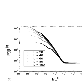
Figure 6: (a) The persistence probability $P(t,L)$ is plotted against time $t$ for different lattice sizes $L$. (b)The scaling function$f(x)=P(t,L)L^{z\theta}$ is plotted against dimensionless scaling variable $x=tL^{-z}$. The data for different $L$ values were found to collapse for longer times for $z=1.62$.

As stated by Fuchs et. al.haye2 (2008), a finite 1+1 dimensional contact process at criticality reaches the absorbing state within finite time so that there is a finite probability for persistent sites to survive forever. Therefore, persistence probability saturates at a constant value. One can easily carry this analogy to non spreading regime in coupled evolution of delayed circle maps in localized chaos regime. When the dynamics is such that no site is laminar, the persistence decays to zero. The scaling function at criticality $\Delta=0$ for various system sizes L, i.e. plotting $P(t)L^{\theta z}$ against $t/L^{z}$, shows a excellent data collapse at longer times for $z=1.62$ and $\theta=1.31$ in Fig. 6.

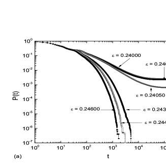
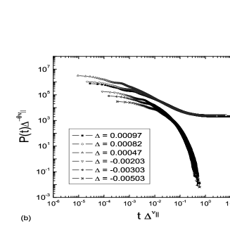
Figure 7: (a) The persistence probability $P(t,L)$ is plotted against time $t$ for different coupling strengths $\epsilon$. (b) The scaling function$f(x)=P(t)\Delta^{-\theta\nu_{||}}$ is plotted against dimensionless scaling variable $x=t\Delta^{\nu_{||}}$. A good data collapse is obtained for $\nu_{||}=1.51$.

Figure 8: (a) Persistence probability $P(t)$ is plotted as a function of time $t$ on a logarithmic scale for $k=1$, $\omega=0.062$ and $\epsilon=0.26634$. The lattice size is 5000. The persistence exponent $\theta=1.2$.

For a continuous phase transition below (above) the critical point, we expect the persistence probability to saturate (decay exponentially). According to above scaling form, the curves should collapse in both cases when $P(t)\Delta^{-\theta\nu_{||}}$ is plotted against $t\Delta^{\nu_{||}}$. This is indeed the case as shown in Fig. 7. The simulations were carried out for lattice size $L=5000$. The size is large enough so that finite size corrections could be neglected. Also ensemble averaging has been performed over 5000 different initial conditions to ensure convergence. Persistence acts as an excellent order parameter for transition from spreading to nonspreading regimes. This point can further be substantiated by similar power law decay seen for $\delta=0$ case of spatial intermittency, as seen by Jabeen and Gupte gupte74 (2006). Figure 8 shows persistence probability behavior for parameter values of coupled circle map without feedback where spatial intermittency is seen. The persistence exponent observed is $1.2$. We would like to note that persistence exponent obtained in transition from laminar state to spatiotemporal chaos (shown to be in DP universality class) is found to $1.5$ menon (2003) while in transition from laminar state to traveling wave state in negatively coupled circle maps, the exponent is $1$ gade (2007). Thus the exponent is clearly different from the exponents observed in previously studied transitions. However as noted previously in literature, persistence is known to be least universal exponent among various dynamical exponents.

V Stability Analysis

Computing Jacobian matrix of the system is useful from several viewpoints. Lyapunov exponents are essentially related to eigenvalues of product of Jacobians over infinite period. For a synchronized or periodic solutions, one can get considerable simplifications by analyzing the Jacobian matrix for those states. The localized state has been previously observed in coupled circle maps by Jabeen and Gupte gupte74 (2006) and has been named as spatial intermittency and they observed certain differences between eigenvalue distributions of one-step Jacobian matrix. It has been observed that eigenvalue spectrum of the Jacobian of the system at any time $T$ gives a good indicator of this phase. We show that the eigenvalues remain real for our systems as well. This spectrum shows distinct features in the phases concerned.

For $\tau=1$, our equations can be put in the form.

$$x_{i}(t+1) = (1-\epsilon-\delta)f(x_{i}(t))\;+\;{\frac{\epsilon}{2}}\;[f(x_{i-1}(t))$$

$$+f(x_{i+1}(t))]+\delta f(y_{i}(t))$$

$$y_{i}(t+1) = x_{i}(t)$$

The Jacobian $J_{t}$ at time $t$ is given by,

$$\mathbf{J_{t}}=\left(\begin{array}[]{cc}A_{t}&B_{N}\\ I_{N}&0_{N}\end{array}\right)$$

where $0_{N}$ is an $N\times N$ Null matrix with all entries $0$. $I_{N}$ is $N$-dimensional identity matrix. The matrix $B_{N}$ is defined as $B(i,i)=\delta f^{\prime}(y_{i}(t))$ and $B(i,j)=0$, if $i\neq j$. The matrix $A_{t}$ is given by,

$$\mathbf{A_{t}}=\left(\begin{array}[]{ccccc}\epsilon_{s}f^{\prime}(x_{1}(t))&\epsilon_{n}f^{\prime}(x_{2}(t))&0&\ldots&\epsilon_{n}f^{\prime}(x_{N}(t))\\ \epsilon_{n}f^{\prime}(x_{1}(t))&\epsilon_{s}f^{\prime}(x_{2}(t))&\epsilon_{n}f^{\prime}(x_{3}(t))&\ldots&0\\ 0&\epsilon_{n}f^{\prime}(x_{2}(t))&\epsilon_{s}f^{\prime}(x_{3}(t))&\epsilon_{n}f^{\prime}(x_{4}(t))&\ldots\\ \vdots&\vdots&\vdots&\vdots&\vdots\\ \epsilon_{n}f^{\prime}(x_{1}(t))&0&\ldots&\epsilon_{n}f^{\prime}(x_{N-1}(t))&\epsilon_{s}f^{\prime}(x_{N}(t))\\ \end{array}\right)$$

where, $\epsilon_{s}$ = $1-\epsilon-\delta$, $\epsilon_{n}=\frac{\epsilon}{2}$ and $f^{\prime}(x_{i}(t)$ = $1-Kcos(2\pi x_{i}(t))$. where, $x_{i}(t)$ is the state variable. The diagonalization of $J_{t}$ gives the $2N$ eigenvalues of the stability matrix. The eigenvalues of the stability matrix were calculated for values of state variable $x_{i}(t)$ for all $i$ at one time step on discarding sufficiently long transients.

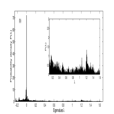
Figure 9: The eigenvalue distribution for (a) $\epsilon=0.2$, (b) $\epsilon=0.3$ is plotted for 50 different realizations for lattice size $L=1000$ with bin-width = 0.001. Gaps are seen in localized chaos eigenvalue distribution whereas the eigenvalue distribution for Spatiotemporal chaos region shows no such gaps. The inset in figure (a),(b) show the magnified region of respective plots

.

Fig. 9(a) shows that the eigenvalue distribution for $\epsilon=0.2$, where spatial intermittency or localized chaos is seen. This distribution has gap or zero probability regions in the eigenvalue spectrum as reported earlier by Jabeen et al. gupte74 (2006). On the other hand, Fig. 9(b) shows that there is no such gap for coupling values $\epsilon=0.3$ where fully grown spatiotemporal chaos is seen. Consider matrix $J_{t}^{\prime}$ given by

$$\mathbf{J^{\prime}_{t}}=\left(\begin{array}[]{cc}A^{\prime}_{t}&B^{\prime}_{N}\\ B^{\prime}_{N}&0_{N}\end{array}\right)$$

where $B^{\prime}(i,i)=\sqrt{\delta f^{\prime}(y_{i}(t))}$ and $B^{\prime}(i,j)=0$, if $i\neq j$. The elements of the matrix $A^{\prime}$ are $A^{\prime}(i,i)=A(i,i)$ and $A^{\prime}(i,j)=\sqrt{A(i,j)A(j,i)}$ which can be obtained from the transformation $A^{\prime}(t)=C^{\prime}AC^{\prime-1}$ where matrix $C^{\prime}(i,i)=\sqrt{\epsilon_{n}f^{\prime}(x_{i}(t))}$.

One can verify that $B^{\prime 2}=B$. Thus, it is easy to see that matrix $J^{\prime}(t)$ and matrix $J(t)$ have same characteristic polynomial and hence they have same eigenvalues. $\displaystyle\left(\begin{array}[]{cc}C^{\prime}&0\\ 0&C^{\prime}B^{\prime}\end{array}\right)$ is the similarity transform which relates $J_{t}$ and $J^{\prime}_{t}$. Now the matrix $J^{\prime}(t)$ is symmetric and has real eigenvalues. Thus, the matrix $J(t)$ also should have real eigenvalues. The assumption has been that $f^{\prime}(x_{i})\geq 0,f^{\prime}(y_{i})\geq 0$ which is justified for $k\leq 1$. The feedback strength $\delta$ is already assumed to be positive in our work. Thus $A(t)$ and $A^{\prime}(t)$ as well as $J_{t}$ and $J^{\prime}_{t}$ are related by similarity transformation and since $A^{\prime}(t)$ and $J_{t}^{\prime}$ are symmetric, $A(t)$ and $J_{t}$ should have real eigenvalues. Thus we can look for gap in eigenvalue spectrum for these matrices and we observe the gap in our case for $\tau=1$. Gupte and Jabeen already noticed the gap for case without feedback. We would also like to note that these are stretching transformations and eigenvectors which are localized in one frame of reference remain localized in other frame of reference as well. This observation will be useful in later section. Thus it is possible to look for gap in the eigenvalue spectrum even in this case. Unfortunately the argument breaks down for $\tau>1$ footnote3 .

Now let us try to understand the reason for gap in eigenvalue spectrum in $A(t)$ in Jabeen and Gupte’s case. We choose a diagonal part of matrix as an unperturbed matrix and all off-diagonal entries as a perturbation. Our choice for $l^{th}$ eigenvector for the diagonal part is a vector whose $l^{th}$ component is unity and all other components are zero. We define $A^{\prime}_{t}=A^{d}_{t}+A^{p}_{t}$, where diagonal entries of $A^{d}_{t}$ are given by $A^{d}_{t}(i,i)=A_{t}(i,i)$ and rest of its entries are zero. Let us consider an idealized case in which $k^{th}$ and $N^{th}$ sites are turbulent and all other sites are laminar. Similar analysis can be carried out for more that two turbulent sites as long as they are not adjacent sites.

$$\mathbf{A^{\prime}_{t}}=\left(\begin{array}[]{cccccccccc}a&b&0&0&0&0&0&\ldots&0&b_{N}\\ b&a&b&0&0&0&0&\ldots&0&0\\ \vdots&\vdots&\ddots&\vdots&\vdots&\vdots&\vdots&\ldots&0&0\\ 0&0&\ldots&a&b_{k}&0&0&\ldots&0&0\\ 0&0&\ldots&b_{k}&a_{k}&b_{k}&0&\ldots&0&0\\ 0&0&\ldots&0&b_{k}&a&b&\ldots&0&0\\ \vdots&\vdots&\vdots&\vdots&\vdots&\vdots&\vdots&\ddots&\vdots&\vdots\\ 0&0&0&0&0&0&0&\ldots&a&b_{N}\\ b_{N}&0&0&0&0&0&0&\ldots&b_{N}&a_{N}\\ \end{array}\right)$$

where $a=(1-\epsilon)f^{\prime}(x^{*})$, $b=\epsilon_{n}f^{\prime}(x^{*})$ and $a_{i}=(1-\epsilon)f^{\prime}(x_{i})$, $b_{i}=\epsilon_{n}\sqrt{f^{\prime}(x_{i})f^{\prime}(x^{*})}$, where $i=k$ and $N$ sites respectively. The matrix $A^{d}_{t}$ has eigenvalue $a$ with $(N-2)$ fold degeneracy and two nondegenerate eigenvalues given by $a_{k}$ and $a_{N}$. The perturbation is $A^{p}_{t}=A^{\prime}_{t}-A^{d}_{t}$. If all sites are laminar except $k^{th}$ and $N^{th}$ site (since we have periodic boundary conditions, by appropriate relabeling of sites, one can always bring the site in turbulent state to $N^{th}$ site), the matrix $A^{d}_{t}=diag(a,a,a_{k}\ldots,a,a_{N})$ , the perturbation will be,

$$\mathbf{A^{p}_{t}}=\left(\begin{array}[]{cccccccccc}0&b&0&0&0&0&0&\ldots&0&b_{N}\\ b&0&b&0&0&0&0&\ldots&0&0\\ \vdots&\vdots&\ddots&\vdots&\vdots&\vdots&\vdots&\ldots&0&0\\ 0&0&\ldots&0&b_{k}&0&0&\ldots&0&0\\ 0&0&\ldots&b_{k}&0&b_{k}&0&\ldots&0&0\\ 0&0&\ldots&0&b_{k}&0&b&\ldots&0&0\\ \vdots&\vdots&\vdots&\vdots&\vdots&\vdots&\vdots&\ddots&\vdots&\vdots\\ 0&0&0&0&0&0&0&\ldots&0&b_{N}\\ b_{N}&0&0&0&0&0&0&\ldots&b_{N}&0\\ \end{array}\right)$$

We perform a simple degenerate state perturbation theory to our perturbation matrix $A^{p}_{t}$, we can consider a matrix $P$ of $(N-2)$ eigenvectors of degenerate eigenvalues as,

$$\mathbf{P}=\left(\begin{array}[]{cccccccc}1&0&0&0&0&0&0&0\\ 0&1&0&0&0&0&0&0\\ \vdots&\vdots&\ddots&\vdots&\vdots&\vdots&\vdots&\vdots\\ 0&0&0&1&0&0&0&0\\ 0&0&0&0&0&0&0&0\\ 0&0&0&0&1&0&0&0\\ 0&0&0&0&0&1&0&0\\ \vdots&\vdots&\vdots&\vdots&\vdots&\vdots&\ddots&\vdots\\ 0&0&0&0&0&0&0&1\\ 0&0&0&0&0&0&0&0\\ \end{array}\right)$$

it can be seen that

$$\mathbf{P^{T}A^{p}_{t}P}=\left(\begin{array}[]{ccccccc|ccccccc}0&b&0&0&\ldots&0&0&0&0&0&0&\ldots&0\\ b&0&b&0&\ldots&0&0&0&0&0&0&\ldots&0\\ 0&b&0&b&\ldots&0&0&0&0&0&0&\ldots&0\\ 0&0&b&0&\ddots&0&0&0&0&0&0&\ldots&0\\ \vdots&\vdots&\vdots&\ddots&\ddots&\vdots&\vdots&\vdots&\vdots&\vdots&\vdots&\ldots&\vdots\\ 0&0&0&0&\ldots&0&b&0&0&0&0&\ldots&0\\ 0&0&0&0&\ldots&b&0&0&0&0&0&\ldots&0\\ \hline\cr 0&0&0&0&\ldots&0&0&0&b&0&0&\ldots&0\\ 0&0&0&0&\ldots&0&0&b&0&b&0&\ldots&0\\ 0&0&0&0&\ldots&0&0&0&b&0&b&\ldots&0\\ 0&0&0&0&\ldots&0&0&0&0&b&0&\ddots&0\\ \vdots&\vdots&\vdots&\vdots&\vdots&\vdots&\vdots&\vdots&\vdots&\vdots&\ddots&\ddots&b\\ 0&0&0&0&\ldots&0&0&0&0&0&0&b&0\\ \end{array}\right)$$

This gives us for each $(N-2)$ fold degenerate eigenvector, a $(N-2)\times(N-2)$ matrix of perturbation $A^{p}_{t}$. We can see that the above matrix contains two blocks. The first block is of $(k-1)\times(k-1)$ size and the second block has size $(N-k-1)\times(N-k-1)$. The eigenvalues of this matrix will be first order corrections. The perturbed eigenvalues after first order perturbation for degenerate states in this case will be,

$$\lambda_{l}=a+2b\cos(\theta_{l})$$ (6)

where toeplitz (2008),

$$\theta_{l}=\left\{\begin{array}[]{lll}\frac{l\pi}{(k-1)+1}&\text{for }l=1,..,k-1\\ \frac{l\pi}{(N-k-1)+1}&\text{for }l=1,..,(N-k-1)\end{array}\right.$$ (7)

We have two non-degenerate eigenvectors, an unit vector in $N^{th}$ direction $v_{N}=[0,0,\ldots,1]^{T}$ and an unit vector in $k^{th}$ direction $v_{k}=[0,0,\ldots 1,\ldots,0]^{T}$. Now $v_{N}^{T}A_{t}^{p}v_{N}=v_{k}^{T}A_{t}^{p}v_{k}=0$. Thus the eigenvalues $a_{k}$ and $a_{N}$ are unperturbed after first order perturbation. Now if these values are far from $a\pm 2b$, we will observe a gap in the spectrum.

Now let us generalize this argument to finite fraction $f$ of turbulent sites. The number of turbulent sites is $m=fN$ and they are interspersed in the lattice. We also assume that no two turbulent sites are adjacent. In that case, we have $a_{i}=(1-\epsilon)f^{\prime}(x_{i})$, $b_{i}=\epsilon_{n}(f^{\prime}(x_{i}))$, where $i=l_{1},l_{2},l_{3},...,l_{m}$ sites respectively, where $l_{1},l_{2},..,l_{m}$ are indices of $m$ turbulent sites and $l_{m}$ site is $N^{th}$ site which can be obtained due to periodic boundary conditions. Again the matrix $A^{d}_{t}$ will have eigenvalue $a$ with $(N-m)$ fold degeneracy and $m$ nondegenerate eigenvalues given by $a_{1},a_{2},...,a_{m}$. The matrix $P$ becomes matrix of $(N-m)$ eigenvectors of degenerate eigenvalues. The matrix of perturbation $A^{p}_{t}$ changes accordingly to $(N-m)\times(N-m)$. We can see that the matrix obtained from operation $P^{T}A^{p}_{t}P$ contains $m$ blocks. The square blocks will be of corresponding size, i. e. for $l_{1}$, the size will be $(l_{1}-1)$, for $l_{2}$ it is $(l_{2}-l_{1}-1)$ and in the same way for $m^{th}$ block corresponding to turbulent site $l_{m}$, the size will be $(l_{m}-l_{(m-1)}-1)$. The generalized case for $m$ turbulent sites goes as,

$$\theta_{l}=\left\{\begin{array}[]{lll}\frac{l\pi}{l_{1}}&\text{for }l=1,..,l_{1}-1\\ \frac{l\pi}{l_{2}-l_{1}}&\text{for }l=1,..,l_{2}-l_{1}-1\\ \frac{l\pi}{l_{3}-l_{2}}&\text{for }l=1,..,l_{3}-l_{2}-1\\ \frac{l\pi}{l_{4}-l_{3}}&\text{for }l=1,..,l_{4}-l_{3}-1\\ \frac{l\pi}{l_{m}-l_{(m-1)}}&\text{for }l=1,..,l_{m}-l_{m-1}-1\\ \end{array}\right.$$ (8)

In any case the eigenvalues are between $[a-2b,a+2b]$. Now let us look at nondegenerate states. Arguing similar to the case of two site, after first order perturbation, the eigenvalues are $a_{l_{1}},a_{l_{2}},\ldots a_{l_{m}}$. If these eigenvalues are not within the range $a\pm 2b$, we will observe a gap in the spectrum. Thus, we predict that eigenspectrum of $J_{t}$ will be given by a band of eigenvalues between $a+2b$ and $a-2b$ superposed with values $\epsilon_{n}(f^{\prime}(x_{j}))$, where $j$ is a turbulent site. Localized eigenstates for $A^{\prime}(t)$ will also be localized for $A(t)$ since they are related by stretching transformation. If we make the histogram of eigenvalues as shown in figure 10, we find that this is indeed true. We can see histograms of eigenvalues computed numerically and theoretically from the eqns. 6 and 8 obtained by pertubative analysis for $20$ turbulent sites in the lattice of $100$ elements. The values for turbulent sites given by $\epsilon_{n}f^{\prime}(x_{j}))$ can also be seen away from the band $[a-2b,a+2b]$. For general case, there is a band of eigenvalues followed by $m$ non-degenerate eigenstates which are far from the band. We checked that these eigenstates are localized and the corresponding eigenvectors are demonstrated in Fig. 11 for case of two turbulent sites.

On the other hand, for spatiotemporal chaos, we have a symmetric random matrix $A^{\prime}_{t}$ which has nonzero entries on diagonal, upper diagonal, lower diagonal and elements $A^{\prime}_{t}(1,N)$ and $A^{\prime}_{t}(N,1)$. In this case, ratio of width of band to system size tends to zero as $N\rightarrow\infty$. The eigenvalue spectrum of such a matrix tends to standard Gaussian distribution liuwang (2009). It is worth noting here that, persistence acts as a good order parameter for this transition for all values of $\tau$ including $\tau=0$, whereas it is not clear that dynamic characterizer of gaps in eigenvalues spectrum might work for higher value of $\tau$.

Table 1: Table showing Eigenvectors showing peaks at corresponding two turbulent sites in otherwise steady state, here $300$ and $500$. In second column larger eigenvalues are given which match with the values shown in last column.

$i$	Eigenvector	Eigenvalue	$(1-\epsilon)f^{\prime}(x)$
500	1	1.0861	1.0817
300	2	0.4177	0.4132

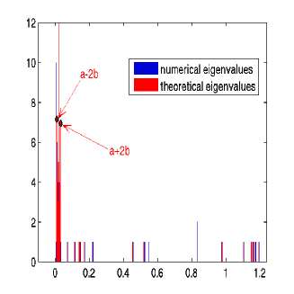
Figure 10: (Color online) Overlapping histograms of the calculated eigenvalues. In red (gray), histogram of eigenvalues obtained by theory of pertubative analysis. In blue(black), histogram of numerically obtained eigenvalues of matrix $A(t)$ is given. The values for turbulent sites given by $\epsilon_{n}f^{\prime}(x_{j}))$ can also be seen away from the band $[a-2b,a+2b]$. The agreement between theory and numerics can be clearly seen for degenerate as well as non-degenerate eigenvalues.

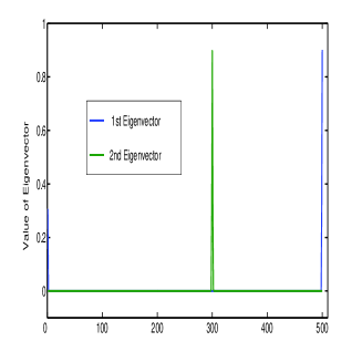
Figure 11: The localized eigenvectors showing peaks at $300$ and $500$ for lattice size $500$.

.

Similar calculations can be carried out for our Jacobian $J^{\prime}_{t}$. The localized eigenvectors explain why localized patterns are stable. The eigenvectors having largest eigenvalue are localized. Thus any perturbation from laminar state is likely to be growing in the direction of localized eigenvectors which does not disturb values at nearby sites. The above analysis of eigenvalue distribution for localized chaos is restricted to demonstrate the analogy to spatial intermittency. The eigenvalue spectrum clearly differentiates infective to non-infective phase. The above analysis explains why the eigenvalue spectrum is different for spatiotemporal chaos and spatial intermittency. footnote4

VI Discussion

In this paper, we have simulated coupled circle maps with feedback. This allows us to study coupled systems where local dynamics is high dimensional. We give an overall phase diagram and discuss various dynamical phases. We also give an all-site bifurcation diagram and remark that there are phases which can not be found from bifurcation diagram and we need to study a detailed simulated space-time plot. In particular, we make a detailed study of a dynamical phase transition between the phase of localized chaos and spatiotemporally chaotic state. We find various characteristics such as distribution of domains of turbulent sites. Phase transition from different dynamical phases is demonstrated. We make an attempt to analyze this transition in a manner in which equilibrium transitions are analyzed. In order that we are able to do so, it is necessary to define an order parameter. We find that local persistence acts as an excellent order parameter to characterize the phase transition. In addition to this, conventional scaling laws pertaining to finite size simulations and offcritical scaling add credibility to use of persistence as quantifier of the transition. Interestingly, same definition of persistence used for without feedback case menon (2003) works for our case with feedback. We also calculate one step Jacobian of the system and find gaps in eigenvalue distribution of system which is dynamical signature of non-infectious nature of dynamics in ‘localized chaos’ regime. The important effect of feedback is that the parameter window for which spatial intermittency is seen, gets enhanced. It should be noted that persistence acts as a good order parameter for this transition for all values of $\tau$ including $\tau=0$, whereas it is not clear that dynamic characterizer of gaps in eigenvalues spectrum might work for higher value of $\tau$. We get this transition for several values of $\tau$. We have shown that persistence acts as an excellent order parameter for this transition for all values of $\tau$. We also try to study gaps in the eigenvalue spectrum which work well for $\tau=0$ and $\tau=1$. We go a step ahead in explaining the origin of such gaps in eigenvalues spectra of one step Jacobian by perturbation theory analysis. Analytical work also gives an idea of when above analysis may not work.

There is a possibility to experimentally investigate dynamical phases in spatiotemporal systems. Certain electrical oscillators are well simulated with circle maps afraimovich (1994); kurths (2002) and it is relatively easy to implement feedback mechanism in electric devices. If one can define a persistence in an analogous manner in differential equations, it is possible to find persistence in spatiotemporal systems experimentally.

In context of localized chaos, we would also like to point to an interesting work by Sethia et. al. Sethia (2008) where they observe ‘chimera’ states, first observed by Kuramoto kuramoto (2002). These states have spatially disconnected regions of synchronization separated by regions of decoherence. Thus there is a strong analogy between ‘chimera’ states and ‘localized chaos’. Several works study ‘chimera’ under various modifications for identical oscillators.abrams (2004); tass (2008); sheeba (2009); wiley (2008) and non-identical oscillators laing (2009). Coupled evolution of systems with delay induces effectively nonlocal contributions in the evolution of individual system. Feedback propagates in space and time and affects the dynamics at some distant site. It could be of interest to find some general definition of persistence applicable to these systems and investigate transition to ‘chimera’ state as a dynamic phase transition. Further work in this direction is pursued.

ARS would like to thank D.A.E, India and C.S.I.R, India for financial support and Dr. S. Barve for useful discussions. PMG would like to thank DST for financial support.

References

- biology (1991) A. J. Koch and H. Meinhardt, Rev. Mod. Phys. 66, 1481 (1991).
- JJA (1988) K. Wiesenfeld, P. Hadley, Phys. Rev. Lett 62, 1335 (1988).
- (3) Bak et al. Solid State Commun. 51,(1984) 231.
- Joseph (1996) K. Wiesenfeld. Physica (Amsterdam) 222(B), 315 (1996).
- rroy (2007) L. Illing, D. J. Gauthier, R. Roy, Adv. in Atomic, Molecular and Opt. Phys. 54, 615 (2007).
- cross (1993) M. C. Cross, P. C. Hohenberg, Rev. Mod. Phys. 65, 851 (1993) and references therein.
- (7) One could also add cellular automata to these list of models. However, we feel that due to discreteness in the value of variables, it displays very different patterns. Usually there is no tunable parameter and bifurcations can not be studied. However, certain patterns in a given cellular automata could look very similar to certain coarse grained patterns in continuous systems
- chate (1988) H. Chate, P. Manneville. Physica D 32, 409 (1988).
- bigazzi (1988) S. Ciliberto, P. Bigazzi, Phys. Rev. Lett 60, 286 (1988).
- barkley (1990) D. Barkley, Nonlinear Structures in Dynamical Systems, edited by Lui Lam and H. C. Moris (Springer-Verlag, New York, 1990).
- reynolds (1990) D. A. Kessler, H. Levine, W. N. Reynolds, Phys. Rev. A 42, 6125 (1990).
- jampa (2007) M. P. K Jampa, A. R. Sonawane, P. M. Gade, S. Sinha, Phys. Rev. E 75, 026215 (2007).
- politi_chaos92 (1992) A. Politi, A. Torcini, Chaos 2(3), 293 (1992).
- bonetto_CUP (2005) F. Bonetto, A. Kupiainen, J. L. Lebowitz, Ergod. Th. & Dynam. Sys. 25, 59 (2005)
- sakaguchi_pre99 (1999) H. Sakaguchi. Phys. Rev. E) 60, 7584 (1999).
- kaneko (1993) K. Kaneko, Theory and Applications of Coupled Map Lattices (Wiley, New York, 1993).
- stanley (1995) A. L. Barabasi, H. Stanley, Fractal Concepts in Surface Growth, (Cambridge University Press, U.K,1995)
- wolf (1996) D. E. Wolf, M. Schreckenberg and A. Bachem, Traffic and Granular Flow, World Scientific, Singapore,1996
- haye (2000) H. Hinrichson, Advances in Physics 49, 815-958 (2000).
- gupte72 (2005) Z. Jabeen and N. Gupte, Phys. Rev. E 72, 016202 (2005).
- gupte74 (2006) Z. Jabeen and N. Gupte, Phys. Rev. E 74, 016210 (2006).
- rahulpandit (2000) A. Pande and R. Pandit, Phys. Rev. E 61, 6448 (2000).
- gade (2007) P.M. Gade, D.V. Senthilkumar, S. Barve, S. Sinha, Phys. Rev. E 75, 066208 (2007).
- ashwini (2010) A. V. Mahajan, P. M. Gade, Phys. Rev. E 81, 056211 (2010).
- ginelli (2003) F. Ginelli, R. Livi, A. Politi, A. Torcini, Phys. Rev. E 67, 046217 (2003).
- Pyragas (1992) K. Pyragas, Phys. Lett. A 170(6), 421-428 (1992).
- handbook (1993) H. Schuster, Handbook of Chaos Control (Wiley-VCH, Weinheim, 1999).
- frozen (1993) F. H. Willeboordse, Phys. Lett. A 183, 187-192 (1993).
- menon (2003) G.I. Menon, S. Sinha, P.C. Ray, Europhys. Lett. 61(1), 27-33 (2003).
- abhijeet_dae (2006) A. R. Sonawane, P. M. Gade, Proc. of DAE Solid State Physics Symposium 51, 129 (2006).
- satya (1999) S. N. Majumdar, Curr. Sci. 77, 370 (1999).
- koduvely (1998) H. Hinrichsen, H. M. Koduvely, Eur. Phys. J. B 5, 257-264 (1998).
- (33) We note that if the number of laminar sites are few and far between which will happen at parameter values extremely close to the transition point, persistence may still go to zero asymptotically since even a small fluctuation will make a non-persistent site persistent. Still, it is fair to say that the critical value at which a power law decay is observed, is very close to, if not the same as, the point at which transition from localized to spatiotemporal chaos occurs. We have checked it by looking at actual pictures for all values of including .
- haye2 (2008) J. Fuchs, J. Schelter, F. Ginelli, H. Hinrichsen, J .Stat. Mech , P04015 (2008).
-
(35)
Notice here that for , the gap in the eigenvalue spectrum
is not a well defined quantity. For e.g. let us consider the case .
Let , , , and . The values
of , and can be arbitrary. Now the Jacobian at first time step is.
which clearly has complex eigenvalues. Thus it is not clear how one is going to look at gaps in eigenvalue spectrum for . - toeplitz (2008) W. Yueh, S. S. Cheng, ANZIAM J. 49, 361-387 (2008).
- liuwang (2009) D. Z. Liu, Z. D. Wang arXiv:0904.2958v2 [math.PR]. , (2008).
- (38) We have not explicitly carried out the stability analysis of synchronized state. However, it can be easily seen that the Jacobian is a block-circulent matrix which can be block-diagonalized to N blocks of size which can easily be diagonalized, see e. g. P. M. Gade and R. E. Amritkar, Phys. Rev. A 47, 143 (1993).
- afraimovich (1994) V. S. Afraimovich, V. I. Nekorkin, G. V. Osipov, V. D. Shalfeev, Stability, Structures and Chaos in Nonlinear Synchronization Networks, (World Scientific, Singapore,1994)
- kurths (2002) G. V. Osipov, A. S. Pikovsky, J. Kurths, Phys. Rev. Lett 88, 054102 (2002).
- Sethia (2008) G. C. Sethia, A. Sen, F. M. Atay, Phys. Rev. Lett 100, 144102 (2008).
- kuramoto (2002) Y. Kuramoto and D. Battogtokh, Nonlinear Phen. in Complex Systems 5:4, 380-385 (2002).
- abrams (2004) D. M. Abrams, S. H. Strogatz, Phys. Rev. Lett 93, 174102 (2004).
- tass (2008) O. E. Omel’chenko, Y. L. Maestrenko, P. A. tass, Phys. Rev. Lett 100, 044105 (2008).
- sheeba (2009) J. H. Sheeba, V. K. Chandrasekar, M. Lakshmanan, Phys. Rev. E 79, 055203(R) (2009).
- wiley (2008) D. M. Abrams, R. Mirollo, S. H. Strogatz, D. A. Wiley, Phys. Rev. Lett 101, 084103 (2008).
- laing (2009) C. R. Laing, Chaos 19, 013113 (2009).