On the cutoff frequency of clarinet-like instruments
Geometrical vs acoustical regularity

Abstract

A characteristic of woodwind instruments is the cutoff frequency of their tone-hole lattice. Benade proposed a practical definition using the measurement of the input impedance, for which at least two frequency bands appear. The first one is a stop band, while the second one is a pass band. The value of this frequency, which is a global quantity, depends on the whole geometry of the instrument, but is rather independent of the fingering. This seems to justify the consideration of a woodwind with several open holes as a periodic lattice. However the holes on a clarinet are very irregular. The paper investigates the question of the acoustical regularity: an acoustically regular lattice of tone holes is defined as a lattice built with T-shaped cells of equal eigenfrequencies. Then the paper discusses the possibility of division of a real lattice into cells of equal eigenfrequencies. It is shown that it is not straightforward but possible, explaining the apparent paradox of Benade’s theory. When considering the open holes from the input of the instrument to its output, the spacings between holes are enlarged together with their radii: this explains the relative constancy of the eigenfrequencies.
PACS: 43.75

1
Introduction

In his paper of 1960, Benade[1] proposed to use the theory of periodic media in order to analyze the effects of a row of tone-holes of wind instruments. He was mainly interested in the length correction at the input of a regular lattice of holes, when they are either all closed or all open. He discovered the existence of an important frequency, the cutoff frequency of the lattice of open holes. Below cutoff, at low frequency (in the stop band), a wave is evanescent, i.e. exponentially decreasing, while above cutoff (in the pass band), it can propagate.

Later, in his book [2], he gave many details about this frequency for real instruments and published experimental results showing the relative independence of this frequency with respect to the fingerings (except the fork ones) in the first register of oboes, bassoons and clarinets. In addition he explained how this frequency is correlated to the tone-color adjectives used by musicians to describe the overall tone of an instrument (see [1] p. 486).
  For a perfectly periodic lattice, the cutoff frequency is independent of the fingering. For real instruments the small variation of the cutoff with respect to the fingering suggests a great regularity of the tone-hole lattice. However this seems to be in contradiction with the great irregularity of the holes of a clarinet. This apparent paradox is the basis of the motivation of the present paper, and was already noticed by Benade in a posthumous article [3]. Comparing 2 clarinets, one with a regular tone hole lattice and an ordinary one, he stated that the input impedances, measured at low level, “were almost identical. This was of course interesting and happy news, because it helped justify the use of formal mathematical physics for a slowly varying lattice on a geometrically quite irregular physical structure”.

Benade proposed a practical method of determination of this frequency based upon the measurement of the input impedance. Two examples will be shown in Figs. 2 and  3. In general, this works properly even for a small number of open holes, thanks to a rather clear distinction between the stop band and the pass band. In principle the measured quantity is a global quantity, related to the input impedance, which a priori depends on the whole geometry of the instrument for a given fingering, i.e. for a given configuration of open holes. It a priori depends therefore on the hole irregularity and the termination of the instrument. As a consequence, the relative independence with respect to fingering is not obvious. Notice that using the measurement of any transfer function, the effect of a (global) cutoff frequency strictly appears only for a periodic, infinite and lossless lattice. When losses exist, the definition is less strict but precise. When the lattice is of finite length or/and irregular, the definition of a global cutoff remains possible in general, as it will be discussed in the present paper. In what follows, we will define the global cutoff frequency as the frequency separating two frequency bands, as viewed on the input impedance curve. It is possible to find an analogy with horn theory: above the global cutoff, the input impedance curve has no resonances.

In his book, Benade also discussed the effect of irregularity. Let us cite him (p. 449): “If the lattice is irregular, theory shows that: (1) if the first and second open-hole segments of the lattice (taken by themselves) have widely different cutoff frequencies, the observed value of $f_{c}$ for the composite system has an intermediate value for its cutoff frequency; and (2) at the lower frequencies, the properties of the first segment still dominate the implications of $f_{c}."$ We can remark that here Benade regards the cutoff frequency as a local quantity, defined for one segment and not for a complete lattice. We will define the local cutoff frequency as the frequency calculated from a given cell (or segment), corresponding to the theoretical cutoff of the periodic medium built with an infinity of cells identical to the considered one. In a paper on cutoff frequencies of flutes, Wolfe and Smith [4] also implicitly considered a local definition (“the cutoff frequency varies from hole to hole”, see Figure 4 of the paper) and calculated it using “typical values” for the dimensions and spacing of holes, in order to use the formula corresponding to a periodic medium. In addition they calculated the deviation of the calculated frequencies, exhibiting a large value for it. (For the classical flute, only the tone holes used in the diatonic scale were included in the means. For the modern instrument, all holes except the trill holes were included).

For a perfectly periodic lattice, i.e. a perfectly geometrically regular lattice, there is no difficulty in defining a local cutoff, because the lattice is divided into identical cells, one cell determining a cutoff. For that case, local and global cutoff frequencies coincide, at least when the lattice is long enough, and the measured global cutoff does not depend on the fingering.

Two questions are examined in the present paper concerning a real instrument, with irregular geometry:

1. Is it possible to define an “acoustical regularity”, for which coincidence between local and global cutoff frequencies is possible even without strict periodicity? We will prove that the answer is positive for a lattice of holes, at least at low frequencies, under the condition that the local cutoff frequency is uniform and the lattice long enough. It will be explained how is possible to build an instrument with this property. This question can be regarded as a direct problem.

2. Concerning the inverse problem, starting from the result of Benade that the global cutoff depends little on the fingering, and on the number of open holes, is it possible to find an “acoustical regularity” in a real clarinet? The answer will be shown to be positive. For this purpose, the delicate problem of the division of a real clarinet into acoustically regular cells needs to be solved. The solution is not simple, as will be shown hereafter.

The final objective of the paper is to compare the obtained local cutoffs to the global ones, where the local cutoffs are calculated from the geometrical dimensions of different holes, while global cutoffs are measured for different fingerings with one or several open holes (for this purpose, it will be be necessary to extend the previous definition of the local cutoff). In general the lattices are with losses and sometimes of short length, and in addition they are not regular, thus the definition of the global cutoff using the input impedance is necessarily done with a non negligible uncertainty. In other words, there is no perfect separation between two frequency bands. Therefore for the sought comparison, an accurate calculation of the local cutoff is not useful and would be illusory. This allows an approximate treatment, with simplification of the model. Nevertheless this leads to a satisfactory comparison with experiment.

The outline of the paper is as follows: section 2 reviews the theory of Benade, and adds a useful interpretation of the cutoff frequency as the eigenfrequency of a cell (i.e. a segment) of the lattice. Section 3 presents experimental results for a Yamaha Y250 clarinet for the global cutoff frequencies measured from the input impedance, confirming Benade’s results. In addition numerical simulation exhibits the important effect of the termination, even for a periodic lattice. Section 4 discusses the first above-mentioned question. Section 5 tries to answer the second question: in a first step, the tube is supposed to be cylindrical and without closed tone holes, and in a second step some corrections are sought to this simplification. In section 6 global and local cutoff frequencies of the clarinet are compared and acoustical regularity is discussed.

2 Periodic lossless lattice of holes: the cutoff frequency and its interpretation as an eigenfrequency

Benade[2] proposed a formula for the first cutoff frequency of a perfectly periodic lattice of open holes, valid at low frequencies (it is recalled below as Eq. (6)). We remark that the corresponding frequency is the eigenfrequency of a Helmholtz resonator built as follows: the volume is that of a portion of the main tube with a length equal to the spacing between two adjacent holes, and the neck is the open tone hole. In this section we review the basic model, and explain why this remark is true, even at higher frequencies. The considered lattice is built with a row of $T$-shaped cells (see Fig.1).

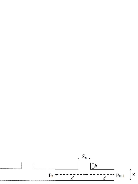
Figure 1: Two $T$-shaped cells of a lattice of tone holes. A T-shaped cell consists of the tone hole and a length $\ell$ of the main tube on both sides of the hole. The cross section areas are $S=\pi a^{2}$ and $S_{h}=\pi b^{2}$, where $a$ and $b$ are the radii of the main tube and the hole, respectively.

Let us consider the classical transfer-matrix description of a symmetrical cell, relating pressures $p_{n}$ and flow rates $u_{n}$ at the extremities (with indices $n$ and $n+1$), as follows:

$$\left(\begin{array}[]{c}p_{n}\\ u_{n}\end{array}\right)=\left(\begin{array}[]{cc}A(\omega)&B(\omega)\\ C(\omega)&D(\omega)\end{array}\right)\left(\begin{array}[]{c}p_{n+1}\\ u_{n+1}\end{array}\right).$$ (1)

The transfer matrix has the following properties: coefficients $A$ and $D$ are equal, because of symmetry, and the determinant is unity, because of reciprocity. We ignore losses, thus $A$ is real, and $B$ and $C$ imaginary (in what follows both visco-thermal and radiation losses are ignored). In an infinite lattice, the travelling waves are

$$p_{n} = p_{0}\exp(\pm n\Gamma)$$

$$u_{n} = u_{0}\exp(\pm n)\text{ \ ,}$$

where $\Gamma$ is the propagation constant. Using Eq. (2) for the two cells ($n-1$, $n$) and ($n$, $n+1$) leads to $\cosh\Gamma=A.$ Therefore at cutoff, $A=\pm 1$, $\Gamma=0$ or $\pi.$ At the cutoff frequency, the complex amplitude of a traveling lattice wave of pressure (respectively of flow rate), is constant from one cell to the next one, with a factor $\pm 1$. For symmetry reasons detailed hereafter, it can be deduced that either the flow rate or the pressure vanishes at the extremities of the cells.

The relationship between pressure and flow rate waves is defined by the characteristic admittance $\mathcal{Y}_{c}$ (or impedance $\mathcal{Z}_{c}=1/\mathcal{Y}_{c}$), given by:

$$\mathcal{Y}_{c}=\frac{\sinh\Gamma}{B}\text{ thus }\mathcal{Y}_{c}^{2}=\frac{A^{2}-1}{B^{2}}=\frac{C}{B}=\frac{C^{2}}{A^{2}-1}.\text{ }$$ (2)

When $\Gamma$ is imaginary (and $\mathcal{Z}_{c}$ real), waves propagate, while if $\Gamma$ is real (and $\mathcal{Z}_{c}$ imaginary), waves are evanescent. The first case corresponds to pass bands, the second one to stop bands.

At cutoff, $A=\pm 1$, thus $BC=0,$ i.e. either $B$ or $C$ vanishes. If $C$ vanishes, $\mathcal{Y}_{c}$ vanishes too. The flow rate being proportional to $\mathcal{Y}_{c}$ for the waves in the two directions, it is zero for any value of $n$, for both an infinite or a finite lattice. Therefore the pressure wave is constant:

$$p_{n}=Ap_{n+1}=\pm p_{n+1}.$$

If $p_{n}=p_{n+1}$, the pressure field is symmetrical, while if $p_{n}=-p_{n+1}$, the pressure field is antisymmetrical. The dual situation, reversing the roles of pressure and flow rate, occurs if $B=0$. Finally the cutoff frequencies are the eigenfrequencies of a cell with either Neumann ($u_{n}=0$, if $C=0$) or Dirichlet ($p_{n}=0$, if $B=0)$ conditions at the extremities.

The next question is the distinction between the first eigenfrequencies satisfying the termination conditions. At low frequencies, for a cell of a tone-hole lattice, the coefficient $A$ is larger than unity , therefore the waves are evanescent and the first cutoff occurs for $A=+1,$ i.e. when either the pressure field or the flow rate field is symmetrical. As it is well known, a Helmholtz resonator has an eigenfrequency very low when its volume is closed, therefore the first cutoff frequency of the lattice, which is the subject of the present paper, corresponds to the Neumann boundary conditions, with a symmetrical pressure field. This is true even if the wavelength at cutoff is not larger than the dimensions of a cell. In Ref. [5] expressions are given for the four types of cutoff frequencies (see also Appendix B of the present paper), with a comparison of the first four ones, confirming the fact that the lowest cutoff is that of the Helmholtz resonance of a T-shaped cell. It corresponds to the condition $\mathcal{Y}_{c}=0$, or $C=0$, and this is in accordance with a mathematical analysis done by Benade (in his Eq. 8, the cutoff is obtained when the denominator vanishes [1]). To our knowledge, this interpretation is new.

It can be concluded that considering the transfer matrix or the equivalent circuit of a tone-hole (see Refs [6, 7]), the element corresponding to the antisymmetrical field, which is a series impedance denoted $Z_{a},$ does not appear in the expression of the first cutoff frequency (this is a rigorous result, without any approximation). Nevertheless ignoring this series impedance is not valid at any frequency. In Appendix B, it is shown how this series impedance could be taken into account in order to generalize the present approach, but for the purpose of the paper, simplified models are sufficient and we ignore it.

Now, if the height of the hole chimney is assumed to be much shorter than the wavelength, and if losses are ignored, the effect of the tone hole is reduced to a shunt acoustic mass, denoted $m_{h}$. The coefficients for transfer matrices of a $T-$shaped cell are given by standard acoustic theory:

$$A = D=1-2\sin^{2}k\ell+jYz_{c}\sin k\ell\cos k\ell$$ (3)

$$B = z_{c}\left[2j\sin k\ell\cos k\ell-Yz_{c}\sin^{2}k\ell\right]$$

$$C = z_{c}^{-1}\left[2j\sin k\ell\cos k\ell+Yz_{c}\cos^{2}k\ell\right]\text{ ,}$$

where $Y=(j\omega m_{h})^{-1}$ is the shunt admittance of the hole and $z_{c}=\rho c/S$, the characteristic impedance of the main tube. $\rho$ is the air density, $c$ the sound speed, $S=\pi a^{2}$ the cross-section area of the tube, assumed to be cylindrical, $2\ell$ the spacing between two holes, $\omega$ the angular frequency, and $k=\omega/c$ the wavenumber.

The equation satisfied by the cutoff frequency is given by $C=0$:

$$j\frac{\rho c}{S}\cot k\ell=2j\omega m_{h}\text{ .}$$ (4)

The left-side member is the impedance on both sides of the tone hole, deduced from the Neumann boundary condition, while the right-side member is twice the shunt impedance of the tone hole. The mass $m_{h}$ is the sum of the mass of the planar mode in the hole and of the masses corresponding to the radiation impedance into surrounding space and into the main  tube. It is approximately equal to:

$$m_{h}=\rho h_{t}/S_{h}\text{, with }h_{t}\simeq h+1.6b,$$ (5)

where $h$ is the height of the hole, and $S_{h}=\pi b^{2}$ the cross section area of the hole. Notice that $h_{t}$ is denoted $t_{e}$ by Benade.

Solving Eq. (4) when $k\ell<<1$ leads to the result (Ref. [2]):

$$f_{c}=\frac{c}{2\pi}\frac{1}{\ell}\frac{1}{\sqrt{2m_{h}/m}}=\frac{c}{2\pi}\frac{b}{a}\frac{1}{\sqrt{2\ell h_{t}}}.$$ (6)

where $m=\rho\ell/S$ is the acoustic mass of the portion of the main tube of length $\ell$ (notice that in Eq. (6) the compressibility of air in the main tube appears, via the acoustic compliance $C_{a}=\ell S/\rho c^{2},$ but its inertia does not). The exact value of $h_{t}$ depends on several parameters, such as the undercutting of the hole or the existence of a key pad, but this is not critical for the present study, especially because the cutoff depends on the square root of this mass.

A better approximation for the solution of Eq. (4) is the following (see Refs [8, 9]):

$$f_{c}=\frac{c}{2\pi}\frac{1}{\ell}\frac{1}{\sqrt{2m_{h}/m+1/3}}=\frac{c}{2\pi\ell\sqrt{2(a/b)^{2}h_{t}/\ell+1/3}}.$$ (7)

It is obtained by expanding $\cot k\ell$ to the next order in $k^{2}\ell^{2}$. This gives a condition of validity of Eq. (6):

$$\frac{b^{2}}{a^{2}}<<6\frac{h_{t}}{\ell}\text{ \ \ or \ }\frac{m}{m_{h}}<<6\text{ ,}$$ (8)

If $k_{c}=2\pi f_{c}/c$, this condition is equivalent to: $k_{c}^{2}\ell^{2}<<1$ (the half spacing between two holes is much smaller than the cutoff wavelength, i.e. the elements of the system are lumped). For a clarinet, typical values of the cutoff frequency and length $\ell$ are $1500$ Hz and $10$ mm, thus $k_{c}\ell\sim 0.3$, and the condition is satisfied.

The dimensions and locations of the holes are given in Appendix A (Table 1). Table 2 of the same appendix indicates the first opened holes for the different fingerings.

3 Determination of global cutoff frequencies

Benade[2] proposed a simple method to measure the “global” cutoff frequency of a given instrument, considering the curve of the input impedance modulus. The first two frequency bands generally appear rather clearly: the first one with high and regular peaks, the second one with smaller and irregular peaks. Benade defined the cutoff as the boundary between the two bands. As stated in the introduction, in principle this method is perfect for a perfectly periodic lattice (i.e. regular, lossless and infinite). What happens for a real lattice is discussed hereafter.

The explanation given by Benade (p. 434) is based upon the strong radiation of the holes above cutoff. This can be more detailed: below cutoff, in the stop band (waves are evanescent), the effective length of the tube is very close to the tube cut at the first open hole, thus the frequency interval between resonances is large. Moreover boundary layer losses (which are preponderant in this range) are small, thus the impedance peaks are high.

On the contrary, above cutoff (in the pass band), the effective tube is divided into two portions. The first one is without open holes, while the second one is the open-hole lattice. The phase velocity and characteristic impedance are different in the two portions, thus the impedance peaks are irregular. Moreover boundary-layer losses exist over a large length, and several open holes radiate efficiently. Therefore the peaks are lower than in the stop band. The efficient radiation is due not only to the number of holes radiating, but also to the external interaction between the holes, as shown in Ref. [10].

Benade[2] measured modern and baroque instruments, and found that baroque instruments have lower cutoff frequencies than modern ones. The explanation seems to be evident thanks to the analysis of the previous section: first of all, the holes of baroque instruments are generally narrower than those of modern instruments. In addition baroque instruments are basically diatonic instruments while roughly speaking the basis of modern instruments is more chromatic. Therefore spacings between open holes are larger for baroque instruments than for modern ones. These two facts with the interpretation of the cutoff frequency as the eigenfrequency of a cell viewed as a resonator explain the differences in cutoff frequencies. A consequence is the slightly wider compass of modern instruments, even if it is possible to play notes with frequencies higher than the cutoff (obviously a complementary explanation for the wider compass of modern instruments is the addition of new holes). Otherwise the question of the influence of the cutoff frequency on the sound spectrum has been discussed rather rarely, but Benade and Kouzoupis can be cited [11], as well as Ref. [4] for the flutes. This question is out of the scope of the present paper. Finally the question of the influence of cutoff on directivity of woodwinds has been treated in Refs. [1, 12, 8, 10].

3.1 Measurement results

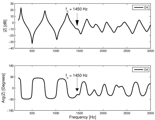
Figure 2: Measured impedance curve for note D4. The cutoff $f_{c}$ is found to be 1450. The scale for the impedance modulus is the logarithmic one: $20\log(|Z|/z_{c}).$

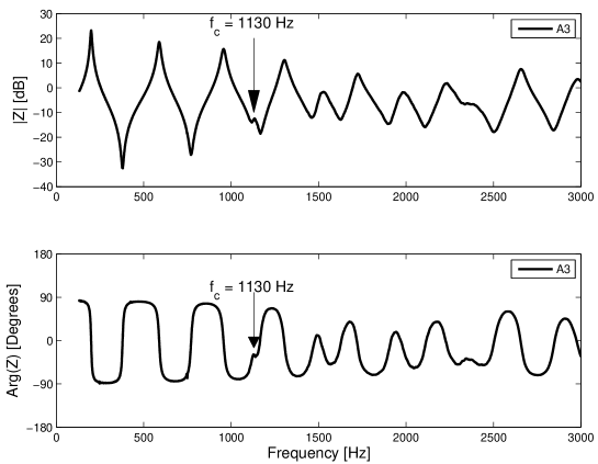
Figure 3: Measured impedance curve for note A3. The cutoff $f_{c}$ is found to be 1130 Hz. The scale for the impedance modulus is the logarithmic one: $20\log(|Z|/z_{c}).$

Benade deduced the cutoff frequency from the measured modulus of the input impedance on a linear scale. Actually it is easier in practice to use either the modulus of the impedance on a logarithmic scale or its argument. This is often better because a slope inversion clearly appears for almost every fingering, even when only a small number of holes is open. This leads to a definition of the global cutoff with a precision in practice better than 1%. Nevertheless, as stated in the introduction, this does not mean that the separation of the two frequency bands is precise, the definition being somewhat arbitrary. A further discussion is given in [13].

Figures 2 and  3  show two examples of measured input impedance curves for the notes D4 and A3. For the note D4 (262 Hz), the global cutoff is found to be 1450 Hz, while for the note A3 it is 1130 Hz. For all the notes of the first register, the measurement of the cutoff frequency is easy, even when only one hole is open (note F3): Benade and Kouzoupis[11] explained this fact by the effect of the bell, “which serves as a more or less surrogate for an open-hole lattice” (sect VIID, see also Ref. [3]).

An interesting result is that the cutoff does not vary very much (a variation of 20% is much smaller than the variations of geometrical dimensions), even for this kind of notes, as it will be seen on Figure 4, which shows the results for the different notes of the clarinet studied (Yamaha Y250). The results are within the range of results obtained by Benade, who measured several different instruments. Notice that Benade gave results for the first register, for the same notes as those we have studied, except the notes for which the first open tone hole is provided with what we call a “closed key”, i.e. a key open for this note only (see Appendix A Table 2). Otherwise, as expected, the cutoff frequencies for the second register, when the register hole is open, are very close to the cutoffs for the first register, for the corresponding fingering.

For the first register, two groups of notes can be observed, above and below B4, around 1450 Hz and 1150 Hz, respectively. We will see in section 3.2 that this difference is not related to regularity, but it is due to the termination effect.

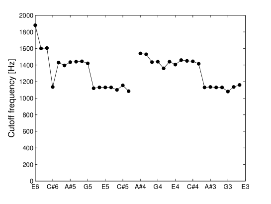
Figure 4: Cutoff frequencies measured for the Yamaha Y250 clarinet. The graph covers all fingerings, and for the first register exhibits a great similarity with the results of Benade, the scale being chosen to be similar.

The device used for the impedance measurement is based upon the measurement of acoustic pressures in two cavities separated by a flow rate source, marketed by CTTM [14].

3.2 Simulation results

In order to get more insight into the problem, some simple simulations using transfer matrices like Eq. (3) have been carried out. No series impedances are taken into account (see Eqs. (3)), but boundary layer losses and radiation, given by standard theory, are considered. Radiation takes external interaction into account, via a global admittance matrix (see Ref. [10]). A simplified shape of the bell is used. Some open holes are considered through a unique, equivalent tone hole, as explained hereafter in section 5.2, resulting in a lattice with 11 open holes. The (global) cutoff frequencies are deduced using the input impedance curve.

Fig.5 shows an interesting qualitative agreement between this model and experiment, sufficient for our purpose. The discrepancy is less than 11%, this value occurring for the note A$\sharp$3. This fact can be related to the location of the limit between the two groups of values, near to A$\sharp$3.

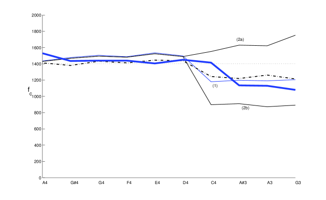
Figure 5: Measured and calculated global cutoff frequencies. Some fingerings are not considered, see explanation in table 2 in Appendix A; moreover the two lowest notes, E3 and F3, are not considered as well, only notes with at least two open holes being considered. Solid, thick line: experimental results (also shown in the previous figure). Dashdot line: numerical result of the simplified model with a bell (see section 5.2.2). Solid, thin lines: numerical results for a purely periodic lattice: (1) with a bell, (2) with a cylindrical tube replacing the bell (for low notes, two possible values of the cutoff are shown, denoted 2a and 2b). The thin, dotted line indicates the theoretical cutoff of the periodic lattice.

The most interesting result is the comparison between the values for the geometrical data of the studied clarinet and those for a perfectly periodic lattice, having 11 open holes with constant spacing $2\ell=0.0341$m and theoretical cutoff $1450$ Hz, the radius being $7.5$ mm. The total length is the same. The common value of the reduced masses, $m_{h}/\rho=340$ m^-1, is deduced from Eq. (6). Notice that the exact value (Eq. (4)) of the theoretical cutoff is $1402$ Hz; the approximation (7), giving also $1402$ Hz, is excellent.

The main features are the following:

• The differences between the results for the purely periodic lattice and the simplified model of the irregular, real one are less than 5%; this can be seen as a first indication of the existence of an acoustic regularity;

• The existence of two groups of values with a limit for A3 is roughly similar for the two lattices;

• Above A3 (first group), when many holes are open, the global cutoff is higher than the theoretical value (1402 Hz), some values being higher than 1500 Hz, the average being 6% higher than the theoretical one. Even for the highest note, when all the holes are open, the global cutoff is 2% higher than the theoretical one.

• The existence of two groups is due to the effect of termination only. This can be checked by replacing the bell by a cylindrical tube of same length and input radius. The values corresponding to the lowest notes (2^nd group) are strongly modified. The above cited sentence by Benade and Kouzoupis is probably true, because for the lowest notes, the determination of the global cutoff is uncertain. For the cylindrical termination, irregular peaks are found around 900 Hz, but the shape of the impedance curves differs strongly from the typical curves shown in Figures 2 and  3.

Figure 6 shows a comparison of theoretical results for two kinds of lattices: the one of the considered clarinet, and the above mentioned periodic latticebell). .

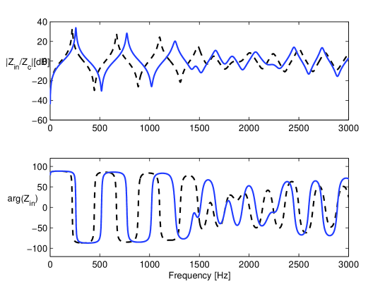
Figure 6: Calculated input impedance curve for the fingering D4. Solid line: simplified model of the clarinet. Dashdot line: periodic lattice of the same length and termination. .

For this particular case, it appears that the practical definition of the global cutoff is easier for the real (irregular) lattice than for periodic one with the same termination. It is a confirmation that the definition of the global cutoff is not always easy in practice (For an infinite lattice without losses, the argument should exhibit a discontinuity between the two bands).

4 Construction of an acoustically regular lattice

This section investigates if acoustically regular lattices can exist. It is known since Anderson[15] that in a onedimensional medium, the effect of an infinite number of random irregularities is the suppression of pass bands, and therefore of cutoff frequencies. Obviously this asymptotic property cannot be observed on musical instruments, because of their limited length. Moreover the theorem of Fürstenberg[16] concerning the product of random matrices indicates that some exceptions to the Anderson’s result can exist. In Ref. [17], it is shown that the product of matrices having the same characteristic impedance $\mathcal{Z}_{c}$ is such an exception. As a matter of fact, for that case:

$$\underset{i}{\overset{N}{\Pi}}\left(\begin{array}[]{cc}\cosh\Gamma_{i}&\mathcal{Z}_{c}\sinh\Gamma_{i}\\ \mathcal{Z}_{c}^{-1}\sinh\Gamma_{i}&\cosh\Gamma_{i}\end{array}\right) = \left(\begin{array}[]{cc}\cosh\sigma&\mathcal{Z}_{c}\sinh\sigma\\ \mathcal{Z}_{c}^{-1}\sinh\sigma&\cosh\sigma\end{array}\right)$$ (13)

$$\text{where \ }\sigma = \underset{i}{\overset{N}{\Sigma}}\Gamma_{i}.$$

The behavior is similar to this of the regular medium with the same total propagation constant $\sigma=n\Gamma$. As a consequence, if a lattice is built with irregular cells having the same characteristic impedance at every frequency, its behavior is the same as the behavior of a perfectly periodic medium. If this situation can exist for wind instruments, acoustic regularity can exist without geometrical regularity. In particular stop and pass bands can exist: when $\sigma$ is imaginary (and $\mathcal{Z}_{c}$ real), waves propagate, while if $\sigma$ is real (and $\mathcal{Z}_{c}$ imaginary), waves are evanescent. This is now investigated.

The cutoff of a $T$-shaped cell is given by $A=1$ or $C=0$ (see Eq. (4)). In order to exhibit the value of the cutoff wavenumber $k_{c}$, using Eq. (4) for $\omega=\omega_{c}$ and $k=$ $k_{c}$, the mass $m_{h}$ can be eliminated and the admittance $Y=(j\omega m_{h})^{-1}$ is rewritten as follows:

$$Y=-2jz_{c}^{-1}\frac{k_{c}}{k}\tan k_{c}\ell\text{ .}$$

Thus, using the definition of the transfer matrix (Eq. (3)):

$$\mathcal{Z}_{c}^{2}=\frac{B}{C}=z_{c}^{2}\frac{1+\frac{k_{c}}{k}\tan k_{c}\ell\,\tan k\ell}{1-\frac{k_{c}}{k}\tan k_{c}\ell\,\cot k\ell}.$$ (14)

The characteristic impedance is written with respect to two quantities, the half-length $\ell$ of a cell and the cutoff wavenumber $k_{c}$, the latter parameter replacing the hole mass. If a lattice is built with cells of identical $k_{c}$, the characteristic impedance can be identical (i.e. independent of $\ell$) at low frequencies if both $k_{c}\ell$ and $k\ell$ are small quantities:

$$\mathcal{Z}_{c}=\frac{B}{C}=z_{c}^{2}\frac{1+O(k_{c}^{2}\ell^{2})}{1-k_{c}^{2}/k^{2}}.$$ (15)

The propagation constant is given by $\sinh^{2}\Gamma=BC$ with

$$BC=-4\sin^{2}k\ell\cos^{2}k\ell\,\;(1+k_{c}k^{-1}\tan k_{c}\ell\tan k\ell)(1+k_{c}k^{-1}\tan k_{c}\ell\,/\tan k\ell)$$ (16)

thus with the same approximation,

$$\Gamma=2j\varphi\ell\text{ \ \ with \ }\varphi=k\sqrt{1-\frac{k_{c}^{2}}{k^{2}}}\text{.}$$ (17)

$\varphi$ is an equivalent wavenumber. Therefore, in the frequency range where the cell dimensions are smaller than wavelength (and consequently where Eq. (6) is valid), it is possible to build an acoustically regular lattice, provided that the cutoff frequency of the cells is a constant. The length of the cells can be arbitrarily chosen but cannot be too long, and for each cell the value of the hole acoustic mass is deduced from the chosen value of the cutoff frequency. Notice that starting from the input of the tube, the distance between holes can either increase or decrease, and consequently the hole masses can decrease or increase, respectively (e.g. the hole radii increase or decrease). The property of the considered lattice is identical to that of a purely periodic one, therefore the global cutoff is the same as the local cutoff of the cells. This is the answer to the first question in the introduction.

Eqs. (15) and (17) suggest an analogy with the problem of an exponential horn: this is discussed in Ref. [5]. Studying the “horn function” of a given bell as Benade did, is equivalent to studying the local cutoff frequency of the bell, which has strong variation for instance for a trumpet bell[18].

This result concerning acoustical regularity will be more complicated if the antisymmetrical (negative) masses are taken into account in the calculation, but the answer remains positive (see Appendix B). Other complications of the model are possible if they can be compatible with the basic model, based upon the association of an acoustic mass with an acoustic compliance. Fortunately this is in general the case at low frequencies.

5 The inverse problem; analysis of an irregular lattice

5.1 Statement of the problem

We will now analyze the lattice of a real instrument. Solving the inverse problem, i.e. dividing a given lattice into cells having the same cutoff frequency, is not an easy task, because the solution either is not unique or does not exist, as explained hereafter. Obviously a first requirement for a method of division is to re-obtain the initial division when considering a lattice built as explained in section 4, instead of a real one.

We first assume the clarinet to be a purely cylindrical tube with holes of different sizes. As it is known, the radius of the main tube does not vary very much for a clarinet. We will see how it is possible to take into account conicity of some portions as corrections. Another hypothesis has been made: in a first step the closed holes have no influence, and their effect is taken as another kind of correction.

For the present purpose, we consider 14 open holes. In three cases (holes number 8 and 9, 14 and 15, 18 and 19, see Appendix A, table 2), two closely spaced holes are opened simultaneously in order to get a given note: according to the basic hypothesis of long wavelength, we choose to replace them by a single hole, with a mass equivalent to the two masses in parallel, and located at the middle of the interval of the two holes. It remains 11 equivalent holes, therefore 11 cells. All the other holes are closed.

Three methods of analysis have been investigated, the first two being based upon different choices of division of the bore into cells, the third trying to extend the definition of a local cutoff frequency without any division.

5.2 Methods of analysis and results

5.2.1 Division into symmetrical cells with varying eigenfrequency

A first method is implemented to divide the tone-hole lattice into $T$-shaped, symmetrical cells. It is not possible to fix a common value for the cutoff frequency, because doing that all the cell lengths become fixed (they are deduced from the values of the hole masses and of the eigenfrequencies), and the cells either will have overlap or do not re-build the complete lattice.

Thus for the chosen method no value for the cutoff is a priori fixed. An initial parameter is arbitrarily chosen, i.e. for instance the half length of the first (upper) cell in the lattice, denoted $\ell_{1}$. Using iteration, this implies the length of each cell, therefore the whole division of the lattice. The cutoff frequencies of each cell can be deduced. They are a priori different, and depend on the chosen value for $\ell_{1}$. The ratio $R_{c}$ of the cutoff highest value to the lowest one is calculated, and the final choice of the parameter $\ell_{1}$ is found by searching for the minimum value of this ratio, which appears very clearly.

The method is first tested on an ideal (acoustically regular) lattice of 11 tone-holes, as defined in the previous section. As expected, the minimum ratio $R_{c}$ is unity, for a length $\ell_{1}$ equal to the half length of the first cell. The method is therefore capable of dividing correctly a lattice built to be acoustically regular.

On the contrary, when applied to the lattice of a clarinet, no division has been found, because negative spacings between holes appear. This is probably due to the close location of the two first upper holes. When ignoring these two holes, a result is found, but the value of the minimum ratio is 2.8: this value is high, while the other approaches, as it will be discussed hereafter, give much smaller values, i.e. a much more uniform value for the cutoff frequencies. Therefore this method has been abandoned [19].

5.2.2 Division into asymmetrical cells with constant eigenfrequency

For the second method, a more general model of acoustically regular lattices is investigated, with one degree of freedom more. Asymmetrical cells are considered: the hole is not necessarily located at the middle of the cell. As a matter of fact, the location of the neck of a Helmholtz resonator has a small influence on its eigenfrequency. The essential elements are an acoustic mass and an acoustic compliance, related to the volume. At low frequencies, it is therefore possible to modify a (symmetrical) $T$-shaped cell by moving the input and output by the same length, $\delta,$ without changing the transfer matrix (the condition being $\delta<<\lambda$, if $\lambda$ is the wavelength). The accuracy of the model based upon this division is a priori similar to that of the division into symmetrical cells (this will be discussed more precisely when comparison with measured global cutoff frequencies will be presented).

The division into asymmetrical cells makes available a supplementary parameter. It is possible to set a constant value for the eigenfrequency of the different cells. From the knowledge of the eigenfrequency and the hole mass, the lengths $\ell_{ln}+\ell_{rn}$ of the cells are obtained. The starting point is an initial value for the length $\ell_{l1}$ to the left of the first open hole. Therefore, from the knowledge of $\ell_{ln}$, the length $\ell_{rn}$ on the right of the hole is deduced, then, from the spacing between two holes, the length $\ell_{ln+1}$, etc.

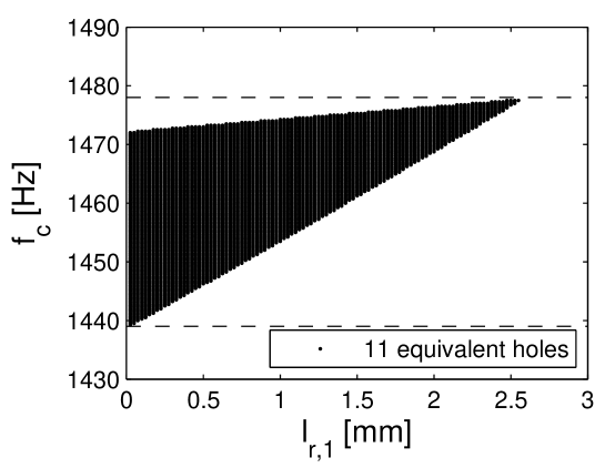
Figure 7: 2^nd method: Division of a lattice with 11 equivalent holes into asymmetrical cells. On the horizontal axis is the semi-cell length to the right $\ell_{r1}$. The region where a solution (i.e. a possible common eigenfrequency) is found is dashed and the horizontal dotted lines limit the frequency range where a correct partition exists.

Depending on the choice of the initial length $\ell_{l1},$ a more or less wide range of possible eigenfrequencies is found. The result is that a solution exists for $f_{c}\in[1439,1478]$ Hz, as shown in Fig.7 (there is a continuum of solutions).

Looking at the partition itself, graphed in Fig.8 for $f_{c}=1470$ Hz and $l_{r,1}=1.50$mm, it is observed that some cells are very asymmetrical, the borders being located very close to the middle of a hole (and even within the hole opening). This seems to be curious and unreal, but formally the transfer matrix of the whole lattice is identical to this of an acoustically regular one, and we will see in the final discussion that the results are interesting. The acoustical regularity can be far from the geometrical one!

The surprise can diminish if we accept that the found lattice is equivalent to the symmetrized lattice with the same holes and cells, but with holes at the center of the cells. We checked that the main discrepancies between the asymmetrical lattice and the symmetrized one occur at frequencies much higher than cutoff. Nevertheless the relative error is non negligible at very low frequencies, and this is intuitive: makers know that the shift of the first open tone hole modifies the first resonance frequencies. Further analytical analysis confirms that the expected error due to the moving of the holes is larger at low frequencies than around cutoff. Finally we notice that this symmetrized lattice cannot be found by the first method, which is not flexible enough.

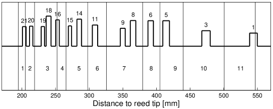
Figure 8: 2^nd method: Illustration of the partition into 11 asymmetrical cells for $f_{c}=1470$ Hz and $l_{r,1}=1.50$mm. The numbers below are the cell numbers from the input of the instrument; while the numbers on the top are the hole numbers, as defined in Appendix A. For three cells, two holes have been replaced by an equivalent hole.

5.2.3 A possible extension of the definition of a local cutoff frequency

A third method of analysis is not based upon any possible division. If two adjacent, symmetrical $T$-shaped cells have the same eigenfrequency with different lengths $\ell_{1}$ and $\ell_{2}$ and different hole masses $m_{h1}$and $m_{h2},$ Eq. (6) leads to:

$$\ell_{1}m_{h1}=\ell_{2}m_{h2}=\frac{\rho}{2Sk_{c}^{2}}\text{ ,}$$ (18)

therefore the spacing $d=\ell_{1}+\ell_{2}$ between the holes satisfies:

$$d=\frac{1}{k_{c}^{2}}\frac{\rho}{2S}\left(\frac{1}{m_{h_{1}}}+\frac{1}{m_{h2}}\right)$$ (19)

thus

$$f_{c}=\frac{c}{2\pi}\sqrt{\frac{\rho}{2Sd}\left(\frac{1}{m_{h_{1}}}+\frac{1}{m_{h2}}\right)}.$$ (20)

This quantity can be calculated without a division of the lattice for every pair of tone holes. It is the eigenfrequency of a resonator of length $d$, with two necks corresponding to the holes with a cross section divided by 2. If it is a constant over the length of a lattice, the lattice is acoustically regular. If it is not constant, its variation can be regarded as a measure of irregularity. We can define the frequency given by Eq. (20) as a local cutoff frequency, depending in a direct way on the dimensions (masses) of two adjacent holes and their distance. This extend the definition given in the introduction, and the two definitions are coherent for either geometrically or acoustically regular lattices.

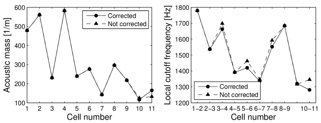
Figure 9: 3^rd method. Left figure: Acoustic mass divided by the density $m_{h}/\rho$, for 11 equivalent tone holes. Right figure: Local cutoff frequency for a pair of adjacent holes (Eq. (20)). For both quantities, the uncorrected and corrected models (see section 5.3) are compared.

Fig.9 shows the results of the third method. An important feature is the difference in variation for the acoustic masses and the local cutoff frequencies. The maximum variation for the square root of the masses is 2.24 while the maximum variation for the cutoff frequencies is 1.38. It can be concluded that the choice of the spacing between the tone holes allows a significant compensation for the variation of the hole acoustic masses, and a certain acoustical regularity exists. This is confirmed by a rough inspection of the holes of a real instrument: the holes appear to be larger as well as their spacing from the input to the bell. Is this effect directly sought by the makers? It is far from evident, and to our minds this remains an open question.

5.3 Results with corrections

The objective of the present work is to analyze a real lattice in terms of acoustical regularity, and implies use of a simple model. Actually many details have an influence on the local cutoff frequencies, but the order of magnitude of this influence remains small. In order to validate this idea, two types of corrections have been studied:

• the effect of closed holes. At low frequencies, this effect is due to the air compressibility, and is proportional to the volume of the cavity of the closed hole. The volume of the portion of the main tube involved in Eq. (6) is therefore modified, in accordance with the lumped elements hypothesis. Fig.9 shows that the correction for the cutoff is small. The cutoff frequency is lowered by a typical amount of 25 Hz.

• the effect of the cross-section variation of the main tube. We are interested in the enlargement of the portion of the tube where open holes are present. This portion is not long. The choice is to describe this enlargement as the insertion of a change in conicity, just below hole n${{}^{\circ}}3$ (see Appendix A), by using results explained e.g. in Ref. [20]. This change in conicity is represented by a supplementary shunt mass $m_{cone}$, which is rather high, i.e. equivalent to a narrow open hole. It is given by the following formula:

  $$m_{cone}=\rho\frac{x}{S}$$

  where $x$ is the length of the missing part of the cone, equal to $287$mm. The mass is inserted at $28.4$mm from hole n${{}^{\circ}}3.$ In addition, the masses of holes n${{}^{\circ}}1$ and n${{}^{\circ}}2$ need to be multiplied by the ratios $S_{1}/S$ and $S_{2}/S$, where $S_{i}$ is the cross section of the main tube at the location of hole n${{}^{\circ}}i.$ Again the correction of the results appears to be very small (see Fig.9).

Concerning the corrections of the results of the 2^nd method of analysis (division into asymmetrical cells), the effect is small as well. The range of possible common eigenfrequencies becomes slightly narrower and lower.

6 Global and local cutoff frequencies

Using the results obtained in the previous section, it is possible to compare the theoretical eigenfrequencies and the measured, global cutoff frequencies. It is reasonable to think that the use of a simplified model does not modify the discussion written hereafter, because the corrections are very small. Nevertheless the results take the two kinds of corrections into account.

Fig.10 shows the results of: i) the measurements of the global cutoffs; ii) the calculation of the possible constant eigenfrequencies using division into asymmetrical cells (2^nd method §5.2.2); iii) the calculation of the local cutoff frequencies (3^rd method, §5.2.3). Notice that there are two different types of axes for the abscissa: for the theoretical results, the numbers correspond to the cell numbers, while for the experimental ones, the results depend on the fingerings.

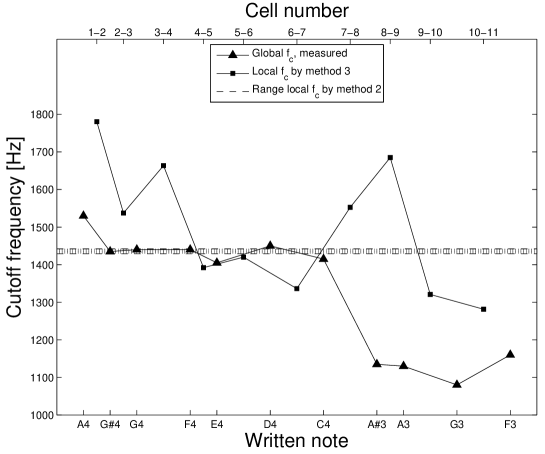
Figure 10: Comparison between experimentally determined global $f_{c}$ and local $f_{c}$ obtained using method 2 and 3 for the corrected model. The values of $f_{c}$ for method 3 are plotted between the tones, because they are based on the acoustic mass of two subsequent equivalent tone holes. The dashed region shows the frequency range for the local $f_{c}$ obtained by the 2^nd method.

The most evident feature is the satisfactory result of the division into asymmetrical cells. The constant eigenfrequency obtained by this method coincides very well with the measured global cutoff for many fingerings. We think that this is a validation of both the definition of the acoustical regularity and the method of division into asymmetrical cells. Nevertheless we notice that this excellent agreement is the consequence of a slight overestimation of the two results: for the theoretical result, as mentioned earlier, the frequency is higher than the true one, because of the use of approximation (6); for the experimental result, it has been seen that the practical measurement of the global cutoff overestimates the true cutoff as well. Otherwise a discrepancy exists for four lower notes. The explanation has been given earlier, in section 3.2, when studying the effect of the termination.

Concerning the 3^rd method, it gives an order of magnitude of the local cutoffs, but they are in general 15% higher than the global measured values, at least at the ends of the considered register. The tendency of the variation looks rather similar, except for fingerings around the note A3 (we have no interpretation of this fact). If for a given fingering the global cutoff was determined by the value of the cell corresponding to the first open hole, the two frequencies should coincide (notice however that the results of this method concern a pair of tone holes). It is not the case, but the fact that the tendency is similar (except for some notes) is in accordance with the hypothesis that the global frequencies are determined by the local frequencies of the first cells.

We finally remark that the 3^rd method seems to be interesting because of its simplicity, no division being needed.  For sake of simplicity, the improvement of Eq. (20) by taking into account the correction term of Eq. (7) is not discussed here. The correction depends on the length of the cell, but the irregularity of the results shown in Fig. 10 is not significantly reduced.

7
Conclusion

A theoretical definition of acoustical regularity is possible, at least at low frequencies, and can be applied to a clarinet. An important degree of acoustical regularity is found on a clarinet, despite the rather great geometrical irregularity. This explains why the measured cutoff frequencies do not vary very much, except when the termination effect occurs. Results for another type of clarinet probably should be rather similar (see especially Ref.[21]).

The acoustical regularity is limited to wavelengths large compared to the inter-hole spacing. A consequence is that if higher cutoff frequencies exist, e.g. limiting a new stop band, the previous analysis of regularity cannot be expected to be relevant for these frequencies. A second stop band seems to exist on both experimental and numerical results between roughly 2500 Hz and 3000 Hz, the second cutoff being different from one fingering to another one. This frequency band was noticed by Wolfe [22]. The understanding of the existence of this band can be a subject for future investigation: what is sure is that it is far from the theoretical next cutoff frequency of the periodic lattice studied in section 3.2. This frequency, called the Bragg frequency in physics, is the half-wavelength eigenfrequency of a cell without holes, i.e. $c/(4\ell),$ equal to 5000 Hz, see e.g. Ref. [8]).

The division of a real lattice as an acoustically regular lattice is not an easy task. Thanks to an extension of the definition of such a lattice, the 2^nd method gives a satisfactory division. Notice that when Benade wrote about the cutoff frequency of segments (in the sentences cited in the introduction), he did not explain how this frequency is defined, i.e. how the two first segments are divided.

The present paper does not present a classical comparison between experiment and theory: a precise comparison between theory and experiment could be sought, especially by taking into account the effect of key pads, the antisymmetrical effects of tone holes, or the precise geometry of the bell. However the agreement between measured global cutoff frequencies and the theoretical cutoff of the acoustically regular lattice built from the real geometry is very good. The limitation to long wavelength is not problematic: this was not evident, because though the spacing between holes is small compared to the cutoff wavelength, the total length of the lattice is not small at all.

The 3^rd method is very simple and gives correct orders of magnitude: the concept is probably rather close to that in the mind of Benade. When qualitatively looking at the location and sizes of the tone holes (see Fig.7), the correlation between larger spacings between holes and wider holes roughly appears, and this is confirmed by the approach of the 3^rd method.

It remains to understand the origin of this correlation. Why do the makers provide an increase of the spacing between holes together with an increase of their radius? Probably it is related to the search for correct tuning, because when a hole is moved downstream, it needs to be enlarged for a given tuning. If this is true, why do the makers enlarge the holes far from the reed? Is it related to radiation efficiency, or to nonlinear effects, or to the possibilities of the fingers and the keys? Another topic for future investigation is a more complete understanding of the effect of the value of the cutoff frequency on the tone color.

In this paper the question of the bell of the clarinet has not been studied in a precise way. Its effect is known to ensure a correct tuning of the second register (see refs [23, 24, 25]). An idea could be that for tone-color purposes, the shape of the bell, which is nearly catenoidal, is sought to be equivalent to a continuation of the open tone-hole lattice. According to Ref. [23], the cutoff of the (infinite) catenoidal horn should be $f=mc/2\pi$, where $m$ is the expansion parameter, found to be $1/0.085$ m${}^{-1}.$ This would lead to a value of $636$ Hz, much lower than the cutoff of the tone-hole lattice. Therefore this simple idea is not satisfactory, and anyway it ignores the finite size effect of periodic media.

Finally we remark that an extension of this study to other cylindrical woodwinds, such as the flute, and even to conical instruments, such as saxophones or oboes, is possible without great complexity.

APPENDICES

Appendix A Geometry of the clarinet studied

The dimensions and locations of the holes of the clarinet Yamaha Y250 are given in Table 1. Table 2 indicates the first opened holes for the different fingerings.

Table 1: Numerical data for the complete set of tone holes. Holes are numbered for decreasing distance to the tip of the reed. Hole 24 is the register hole. Holes 22 and 23 are not used for basic fingerings (see Table 2), therefore they have not been considered in the study. The uncertainties of the measurements are $\pm 0.02$mm for the tone-hole radius, $\pm 0.04$mm for the tone-hole height, and $\pm 0.005$mm for the tube radius.

$no.$	$x$ [mm]	Hole radius $b$ [mm]	Bore radius $a$ [mm]	Hole height $h$ [mm]
24	156.50	1.50	7.53	12.50
23	167.33	2.46	7.50	6.90
22	193.98	2.88	7.46	6.87
21	203.51	2.70	7.46	6.66
20	213.74	2.47	7.46	6.81
19	231.14	2.47	7.46	6.68
18	239.66	3.58	7.47	10.23
17	241.78	2.48	7.47	6.89
16	252.90	2.69	7.47	8.95
15	271.38	2.36	7.47	6.91
14	285.12	3.44	7.47	9.20
13	287.43	2.75	7.47	6.60
12	289.95	2.83	7.47	6.67
11	308.62	3.94	7.47	7.19
10	318.88	2.61	7.47	6.66
9	349.86	3.65	7.49	6.08
8	365.19	4.13	7.51	8.72
7	370.36	3.80	7.52	6.99
6	391.39	4.02	7.54	8.66
5	414.34	4.91	7.55	8.66
4	446.63	5.25	7.53	5.13
3	473.60	6.22	7.52	5.27
2	505.78	5.70	7.67	4.63
1	544.10	5.71	8.40	4.46

Table 2: Most common notes of a B^♭ clarinet (written pitches). The third column gives the target frequency of a well tuned note when it is normally tempered. The fourth column gives the hole number of the first open hole(s) in the lattice. When no number is listed, this note is not considered in this study and does not belong to the “normal” set of fingerings. Excluding a note from this set means that for its corresponding fingering, it is necessary to open a tone hole that keeps closed for the other fingerings.

	Note	$f_{p}$ $[\text{Hz}]$	First opened tone-hole number
Chalumeau	E3	147	all closed
	F3	156	1
	F$\sharp$3	165	-
	G3	175	3
	G$\sharp$3	185	-
	A3	196	5
	A$\sharp$3	208	6
	B3	220	-
	C4	233	8+9
	C$\sharp$4	247	-
	D4	262	11
	D$\sharp$4	277	-
	E4	294	14+15
	F4	311	16
	F$\sharp$4	330	-
Throat	G4	349	18+19
	G$\sharp$4	370	20
	A4	392	21
	A$\sharp$4	415	-
Clarinet	B4	440	all closed
	C5	466	1
	C$\sharp$5	494	-
	D5	523	3
	D$\sharp$5	554	-
	E5	587	5
	F5	622	6
	F$\sharp$5	659	-
	G5	698	8+9
	G$\sharp$5	740	-
	A5	784	11
	A$\sharp$5	831	-
	B5	880	14+15
	C6	932	16

Appendix B Use of a more complete model

We have ignored the negative acoustic masses corresponding to the antisymmetrical field in the holes. If the series impedance $Z_{a}=j\omega m_{a}$ is taken into account together with the shunt admittance $Y=(j\omega m_{h})^{-1}$, the transfer matrix of a hole is written as follows (see e.g Fig.3 of Ref. [7]):

$$\frac{1}{1-Z_{a}Y/4}\left(\begin{array}[]{cc}1+Z_{a}Y/4&Z_{a}\\ Y&1+Z_{a}Y/4\end{array}\right).$$

Multiplying this matrix on both sides by the transfer matrix of a segment of cylindrical tube of length $\ell$ leads to the coefficients of the matrix of the T-shaped cell:

$$B = \left(\cos k\ell+j\frac{Y}{2}z_{c}\sin k\ell\right)\left(Z_{a}\cos k\ell+2jz_{c}\sin k\ell\right)\left(1-Z_{a}Y/4\right)^{-1}$$

$$C = \left(Y\cos k\ell+2jz_{c}^{-1}\sin k\ell\right)\left(\cos k\ell+j\frac{Z_{a}}{2}z_{c}^{-1}\sin k\ell\right)\left(1-Z_{a}Y/4\right)^{-1}.$$

This result exhibits the four types of cutoff frequencies, the lowest one corresponding to the vanishing of the first factor of the coefficient $C$. As expected, all of them depend on either the series impedance or the shunt admittance, for reasons of symmetry. Therefore the exact value of the cutoffs are simpler than those obtained after approximations, as has been done in Ref. [9].

In order to study the acoustical regularity, Eq. (14) is transformed into:

$$\mathcal{Z}_{c}=\frac{B}{C}=z_{c}^{2}\,\frac{1+\frac{k_{c}}{k}\tan k_{c}\ell\,\tan k\ell}{1-\frac{k_{c}}{k}\tan k_{c}\ell\,\cot k\ell}\;\,\frac{1-j\frac{Z_{a}}{2}\cot k\ell}{1+j\frac{Z_{a}}{2}\tan k\ell}.$$

At low frequencies, the characteristic impedance given by Eq. (14) is multiplied by the factor $(1+m_{a}/2m)^{1/2}$. As a consequence, it is possible to ensure an improved acoustical regularity, as follows: in order to obtain a constant characteristic impedance at every frequency, both the cutoff $f_{c}$ and the ratio $(1+m_{a}/2m)/S^{2}$ can be chosen to be equal. Therefore, for a given length $\ell$, there are two equations for the two parameters of the holes (height $h$ and radius $b$).

However the ratio $m_{a}/2m\simeq-0.18b^{3}/(a^{2}\ell$) is in general close to $0.01$ or $0.02$, thus it is not important to take this term into account in the present study, because a high precision is not needed.

References

- [1] A.H. Benade, On the mathematical theory of woodwind finger holes, J. Acoust. Soc. Am. 32(1960), 1591-1608.
- [2] A. H. Benade: Fundamentals of Musical Acoustics. Oxford University Press, London, 1976.
- [3] A.H. Benade and D.H. Keefe. The physics of a new clarinet design. The Galpin Society Journal XLIX (1996), 113-142.
- [4] J. Wolfe and J. Smith : Cutoff frequencies and cross fingerings in baroque, classical, and modern flutes. J. Acoust. Soc. Am. 114 (2003), 2263-2272.
- [5] A. Chaigne, J. Kergomard: Acoustique des instruments de musique. Belin, Paris, 2008.
- [6] D. H. Keefe : Theory on the single woodwind tone hole. J. Acoust. Soc. Am., 72(1982), 676-687.
- [7] V. Dubos, J. Kergomard, A. Khettabi, J. P. Dalmont, D. H. Keefe et C.J Nederveen: Theory of sound propagation in a duct with a branched tube using modal decomposition. Acustica Acta Acustica, 85 (1999), 153-169.
- [8] J. Kergomard: Champ interne et champ externe des instruments à vent. Thèse de Doctorat d’Etat, Université Pierre et Marie Curie, 1981.
- [9] D. H. Keefe: Woodwind air column models. J. Acoust. Soc. Am., 88 (1990), 35-51.
- [10] J. Kergomard: Tone hole external interactions in woodwinds musical instruments, 13th International Congress on Acoustics, Yugoslavia, 53-56, 1989.
- [11] A. H. Benade, S. N. Kouzoupis: The clarinet spectrum : theory and experiment. J. Acoust. Soc. Am., 83(1988), 292-304.
- [12] A.H. Benade. Wind instruments and music acoustics. In “Sound Generation in Winds, Strings, Computers”, No. 29, pages 14-99 (1980),Royal Swedish Academy of Music.
- [13] J. Kergomard, E. Moers, J.-D. Dalmont, Ph. Guillemain: Cutoff frequencies of a clarinet. What is acoustical regularity? Forum Acusticum 2011, 533-538, Aalborg, Denmark.
- [14] C.A. Macaluso, J.-P. Dalmont, Trumpet with near-perfect harmonicity: Design and acoustic results. J. Acoust. Soc. Am. Volume 129 (2011), 404-414.
- [15] P.W. Anderson:Absence of diffusion in certain random lattices. Phys. Rev. 109 (1958), 1492-1505.
- [16] H. Fürstenberg: Noncommuting random matrix products, Trans. Am. Math. Soc. 108 (1963), 377-428.
- [17] C. Depollier, J. Kergomard, F. Laloë, Localisation d’Anderson des ondes dans les réseaux acoustiques unidimensionnels aléatoires, Annales de physique 11 (1986), 457-492.
- [18] A. H. Benade: Physics of Brasses, Scientific American, July 1973, 24-35.
- [19] E.M.T. Moers: Acoustical analysis of the open tone hole lattice of a clarinet. Master Report, Technische Universiteit Eindhoven, Department of Applied Physics, June 2010.
- [20] A. H. Benade: Equivalent circuits for conical waveguides. J. Acoust. Soc. Am., 88 (1988):1764-1769.
- [21] University of New South Wales, http://www.phys.unsw.edu.au/music/clarinet
- [22] University of New South Wales, http://www.phys.unsw.edu.au/jw/cutoff.html
- [23] C.J. Nederveen: Acoustical aspects of woodwind instruments. Northern Illinois University press, 1969.
- [24] C.J. Nederveen, J.P. Dalmont: Corrections to the plane-wave approximation in rapidly flaring horns, Acta Acustica united with Acustica, 94 (2008), 461-173.
- [25] V. Debut, J. Kergomard, F. Laloë, Analysis and optimisation of the tuning of the twelfths for a clarinet resonator, Applied Acoustics 66 (2005), 365-409.
Acknowledgments
We thank Didier Ferrand and Alain Busso for their help for the experiments, and René Caussé, Jean-Pierre Dalmont, Douglas Keefe, Philippe Guillemain, Avraham Hirschberg, Franck Laloë, Kees Nederveen, P.-A. Taillard and Joe Wolfe for useful discussions. We thank also the referees and Murray Campbell for their help in improving the manuscript.