Minimal area ellipses in the hyperbolic plane

Abstract.

We present uniqueness results for enclosing ellipses of minimal area in the hyperbolic plane. Uniqueness can be guaranteed if the minimizers are sought among all ellipses with prescribed axes or center. In the general case, we present a sufficient and easily verifiable criterion on the enclosed set that ensures uniqueness.

1. Introduction and statement of the main result

By a well-known theorem of convex geometry, a full-dimensional, compact subset $F$ of the Euclidean plane can be enclosed by a unique ellipse $C$ of minimal area. We share the general belief that this is an important but easy result. Therefore, it is not surprising that recently much more general uniqueness results were obtained [8, 16, 17]. These articles also contain more complete references to the relevant literature.

The situation in the elliptic plane is different: As of today, uniqueness can only be guaranteed for “sufficiently small and round sets $F$”. The precise statement can be found in [18, Theorem 8]. Its proof requires some non-trivial calculations. It is still an open question whether any compact subset of the elliptic plane possesses a unique enclosing conic or not.

In this article we consider uniqueness of the minimal area ellipse in the hyperbolic plane. The algebraic equivalence of elliptic and hyperbolic geometries suggests to imitate the proof of [18, Theorem 8]. Indeed, this is possible to a large extent, but not completely. The outcome of this research is similar to the elliptic case. Uniqueness can be guaranteed if some conditions on the axis lengths of enclosing ellipses of minimal area are met. If this is not possible, we can make neither a positive nor a negative uniqueness statement. Our main result is

Theorem 1.

Consider a compact and full-dimensional subset $F$ of the hyperbolic plane. The enclosing ellipse of minimal area to $F$ is unique if the following conditions are met:

• There exist positive numbers $\varrho$, $\mathrm{R}$ such that the semi-axis lengths of the (a priori not necessarily unique) minimal ellipses are in the closed interval $[\varrho,\mathrm{R}]$.

• The values $\nu_{1}=\coth^{2}\!\mathrm{R}$ and $\nu_{2}=\coth^{2}\!\varrho$ satisfy the inequality

  (1) $$H(\nu_{1},\nu_{2})\mathrel{\mathop{\mathchar 58\relax}}=-13\nu_{1}^{2}+5\nu_{1}\nu_{2}-3\nu_{1}+7\nu_{2}+4\leq 0.$$

The minimal enclosing ellipse $C_{\min}$ to the convex hull $F$ of a finite point set is depicted in Figure 2. The drawing refers to the Cayley-Klein model of the hyperbolic plane which will be introduced in Section 2.

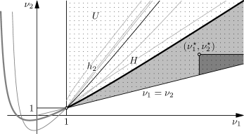
Figure 1. The curves $H(\nu_{1},\nu_{2})=0$ and $h_{2}(\nu_{1},\nu_{2})=0$.

Figure 1 depicts the graph of the function $H(\nu_{1},\nu_{2})=0$. The shaded area contains admissible values $\nu_{1}$, $\nu_{2}$. The meaning of the remaining elements will be explained later in the text.

Condition (1) is certainly fulfilled for $\nu_{1}=\nu_{2}$ and $\nu_{1}\to\infty$. Thus, Theorem 1 informally states that minimal enclosing ellipses are unique if they are sufficiently small and round. Of course, the Theorem should be accompanied by an easily verifiable criterion that ensure suitably shaped minimal ellipses:

Proposition 2.

Consider a compact and full-dimensional subset $F$ of the hyperbolic plane and denote its (hyperbolic) convex hull by $\overline{F}$. Assume $\overline{F}$ admits an inscribed circle of radius $\varrho$ and a circumscribed ellipse of area $S$. Denote by $\mathrm{R}$ the major semi-axis length of an ellipse of area $S$ and minor semi-axis length $r$. Then the minimal area ellipse of $F$ has semi-axis length in the interval $[\varrho,\mathrm{R}]$.

We omit the obvious proof of this proposition. Together with Theorem 1, it leads to the following sufficient test for the uniqueness of the minimal enclosing ellipsoid to a given set $F$:

1. Find a (large) inscribed circle to $\overline{F}$ and denote its radius by $\varrho$.

2. Find a (small) circumscribed ellipse to $\overline{F}$ and denote its area by $S$.

3. Compute the unique value $\mathrm{R}$ such that an ellipse with semi-axis lengths $\varrho$ and $\mathrm{R}$ has area $S$. By construction, $[\varrho,\mathrm{R}]$ is not empty.

4. The minimal area ellipse is unique, if $\varrho$ and $\mathrm{R}$ satisfy the inequality (1).

We will show later that if a point $(\nu_{1},\nu_{2})$ satisfies (1) than the same is true for every admissible point $(\nu^{\prime}_{1},\nu^{\prime}_{2})$ with $\nu^{\prime}_{1}\geq\nu_{1}$ and $\nu^{\prime}_{2}\leq\nu_{2}$. This means, that chances for an affirmative uniqueness statement increase with a large value of the radius $\varrho$ and a small value of the area $S$, that is, with the quality of the input obtained from the first and the second step.

The basic ideas and the initial calculations in our proof of Theorem 1 are more or less identical to the proof of [18, Theorem 8]. The minor differences pertain to occasional changes in sign and the use of the hyperbolic functions $\cosh$, $\sinh$, etc. instead of their spherical counterparts $\cos$, $\sin$, etc. The major differences are in the final estimates. Given the similarities between the elliptic and hyperbolic case, we consider a rather terse presentation appropriate. Yet, we will try to work out the crucial junctions points and the major differences.

In Section 2 we settle our notation and introduce the hyperboloid model of the hyperbolic plane, where our calculations take place. In Section 3 we provide a formula for the area of ellipses in the hyperbolic plane, which is probably hard to find elsewhere. In Section 4, we prove a fundamental convexity result for the area function. By standard arguments, it yields uniqueness of the minimal ellipse among all ellipses with prescribed axes or center. The proof of Theorem 1 is given in Section 5. Its main ingredient is Lemma 7, the Half-Turn Lemma. The merely technical parts of its proof are moved to the appendix.

2. The hyperboloid model of hyperbolic geometry

In [18] we used the spherical model of the elliptic plane for investigating uniqueness of minimal area conics. It is obtained from the geometry of the unit sphere $\mathbb{S}^{2}$ of Euclidean three-space by identifying antipodal points. By analogy, our calculations in this article refer to the spherical model (or “hyperboloid model”) of the hyperbolic plane which is obtained in similar fashion from the geometry of the sphere of squared radius $-1$ in Minkowski three space $\mathbb{R}^{3}_{1}$. An elementary introduction to this model is given in [14].

Minkowski three-space $\mathbb{R}^{3}_{1}$ is the metric space over $\mathbb{R}^{3}$ where the metric is induced by the indefinite inner product

$$\langle x,y\rangle=-x_{0}y_{0}+x_{1}y_{1}+x_{2}y_{2}.$$

The locus of the spherical model of the hyperbolic plane is the sphere $\mathbb{S}^{2}_{1}$, defined as

$$\mathbb{S}^{2}_{1}=\{x\in\mathbb{R}^{3}_{1}\colon\|x\|^{2}=-x_{0}^{2}+x_{1}^{2}+x_{2}^{2}=-1\}.$$

In a Euclidean interpretation, it is a hyperboloid of two sheets. We use $\mathbb{S}^{2}_{1}$ as a model of the hyperbolic plane $\mathbb{H}^{2}$. The following concepts are taken from [14]:

• The points of $\mathbb{H}^{2}$ are the points of $\mathbb{S}^{2}_{1}$ with antipodal points $x$ and $-x$ identified.

• The lines of $\mathbb{H}^{2}$ are the intersections of $\mathbb{S}^{2}_{1}$ with planes through the origin $0$.

• The hyperbolic distance between two points $x$, $y\in\mathbb{S}^{2}_{1}$ is defined by

  $$\operatorname{dist}(x,y)=\operatorname{arccosh}(-\langle x,y\rangle).$$

• The hyperbolic angle between two straight lines $K$ and $L$ is defined by

  $$\sphericalangle(k,l)=\arccos\frac{\langle k,l\rangle}{\|k\|\cdot\|l\|}$$

  where $k$ and $l$ are two arbitrary tangent vectors of $K$ and $L$, respectively.

Note that this model of $\mathbb{H}^{2}$ is closely related to the well-known bundle model and also the Cayley-Klein model of the hyperbolic plane. The bundle model is obtained by connecting points and lines from the spherical model with the origin $0$ of $\mathbb{R}^{3}_{1}$; the Cayley-Klein model is obtained by intersecting the bundle model with the plane $x_{0}=1$. Its points are the inner points of the circle

$$K\colon x_{0}=1,\ x_{1}^{2}+x_{2}^{2}=1.$$

We will occasionally use the Cayley-Klein model for the purpose of visualization but it is also convenient for defining center and axes of an ellipse $C$ in the hyperbolic plane.

The conics in the spherical model of $\mathbb{H}^{2}$ are the intersections of $\mathbb{S}^{2}_{1}$ with quadratic cones centered at $0$. In the Cayley-Klein model, hyperbolic ellipses are conics that lie in the interior of $K$. The ellipse center is the unique vertex $c$ of the common polar triangle $P$ of $C$ and $K$. It is indeed a center in elementary sense, as it halves the (hyperbolic) distance between the ellipse points on any line incident with $c$. The axes of $C$ are the two sides of $P$ through $c$. Degenerate pole triangles characterize the circles among the ellipses. Their center is still well-defined but the axes are undetermined so that any line through $c$ can be addressed as axis. Figure 2 displays a hyperbolic ellipse, its center and axes in the Cayley-Klein model.

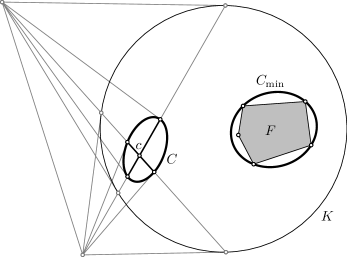
Figure 2. Center $c$ and axes of a hyperbolic ellipse $C$; minimal ellipse $C_{\min}$ to the convex hull $F$ of a finite points set

3. The area of ellipses

The hyperbolic plane $\mathbb{H}^{2}$ can be parametrized as

(2) $$\mathbb{H}^{2}\colon Y(\theta,\varphi)=\begin{pmatrix}\cosh\theta\\ \sinh\theta\sin\varphi\\ \sinh\theta\cos\varphi\end{pmatrix},\quad\theta\in[0,\infty),\varphi\in[-\pi,\pi).$$

A conic $C$, defined as the intersection of this point set with a quadratic cone whose vertex is in the origin, can be described as

$$C=\{x\in\mathbb{H}^{2}\colon x^{\mathrm{T}}\cdot M\cdot x=0\},$$

where $M\in\mathbb{R}^{3\times 3}$ is an indefinite symmetric matrix of full rank. A vector $x$ is called (Minkowski) eigenvector of $M$ with (Minkowski) eigenvalue $\lambda$ if

(3) $$M\cdot x=\lambda I\cdot x.\quad\text{where}\quad I=\operatorname{diag}(-1,1,1).$$

By $e(M)=(\nu_{0},\nu_{1},\nu_{2})$ we denote the vector of eigenvalues of $M$, arranged in ascending order. We will only consider the case where $M$ describes an ellipse. In this case $M$ can be normalized such that $e(M)=(1,\nu_{1},\nu_{2})$ and $1<\nu_{1}\leq\nu_{2}$.

A point $x$ is contained in the ellipse $C$ if it satisfies $x^{\mathrm{T}}\cdot M\cdot x<0$ and $M$ is in normal form. After a suitable (Minkowski) rotation of $\mathbb{S}^{2}_{1}$ we may assume that the ellipse is described by the diagonal matrix

(4) $$M=\operatorname{diag}(-1,\nu_{1},\nu_{2}).$$

Referring to the parametrization (2), points inside $C$ belong to parameter values $(\theta,\varphi)$ related by

$$\theta<\theta^{\star}=\operatorname{arccosh}\sqrt{\frac{\nu_{1}\sin^{2}\!\varphi+\nu_{2}\cos^{2}\!\varphi}{\nu_{1}\sin^{2}\!\varphi+\nu_{2}\cos^{2}\!\varphi-1}}.$$

By integrating the area element

$$\sqrt{\Bigl{\langle}\mathinner{\dfrac{\partial{}H}{\partial{\theta}}},\mathinner{\dfrac{\partial{}H}{\partial{\theta}}}\Bigr{\rangle}\cdot\Bigl{\langle}\mathinner{\dfrac{\partial{}H}{\partial{\varphi}}},\mathinner{\dfrac{\partial{}H}{\partial{\varphi}}}\Bigr{\rangle}-\Bigl{\langle}\mathinner{\dfrac{\partial{}H}{\partial{\theta}}},\mathinner{\dfrac{\partial{}H}{\partial{\varphi}}}\Bigr{\rangle}^{2}}\operatorname{d\!}\theta\wedge\operatorname{d\!}\varphi=\sinh\theta\operatorname{d\!}\theta\wedge\operatorname{d\!}\varphi$$

of (2) (see for example Proposition 5.2 of [3]) we obtain the area of the conic $C$ as

(5) $$\operatorname{area}(C) =\operatorname{area}(\nu_{1},\nu_{2})=\int_{-\pi}^{\pi}\int_{0}^{\theta^{\star}}\sinh\theta\operatorname{d\!}\theta\operatorname{d\!}\varphi$$

$$=\int_{-\pi}^{\pi}(\cosh\theta^{\star}-1)\operatorname{d\!}\varphi=\int_{-\pi}^{\pi}\sqrt{\frac{\nu_{1}\sin^{2}\varphi+\nu_{2}\cos^{2}\varphi}{\nu_{1}\sin^{2}\varphi+\nu_{2}\cos^{2}\varphi-1}}\operatorname{d\!}\varphi-2\pi.$$

This is valid as long as $M$ is normalized such that $e(M)=(1,\nu_{1},\nu_{2})$. If $M$ is not normalized and has ordered eigenvalues $e(M)=(\nu_{0},\nu_{1},\nu_{2})$, the area formula becomes

(6) $$\operatorname{area}(\nu_{0},\nu_{1},\nu_{2})=\int_{-\pi}^{\pi}\sqrt{\frac{\nu_{1}\sin^{2}\!\varphi+\nu_{2}\cos^{2}\!\varphi}{\nu_{1}\sin^{2}\!\varphi+\nu_{2}\cos^{2}\!\varphi-\nu_{0}}}\operatorname{d\!}\varphi-2\pi.$$

4. Convexity of the area function.

Convexity of the area function (5) is already the key property for uniqueness of the minimal area ellipse among concentric or co-axial ellipses. Recall that only values $\nu_{1}$, $\nu_{2}>1$ are admissible.

Lemma 3.

The area function (5) is strictly convex for $\nu_{1}$, $\nu_{2}>1$.

Proof.

We proof that the Hessian matrix of (5) is positive definite, that is, all its principal minors are positive. The upper left entry equals

(7) $$\mathinner{\dfrac{\partial{{}^{2}}\operatorname{area}}{\partial{\nu_{1}^{2}}}}=\frac{1}{4}\int_{-\pi}^{\pi}J\sin^{4}\!\varphi\operatorname{d\!}\varphi,$$

where

$$J=\frac{4\nu_{1}\sin^{2}\!\varphi+4\nu_{2}\cos^{2}\!\varphi-1}{(\nu_{1}\sin^{2}\!\varphi+\nu_{2}\cos^{2}\!\varphi)^{3/2}(\nu_{1}\sin^{2}\!\varphi+\nu_{2}\cos^{2}\!\varphi-1)^{5/2}}.$$

Clearly, $J$ is positive for admissible values of $\nu_{1}$ and $\nu_{2}$. Therefore, (7) is positive as well. The determinant of the Hessian matrix is

(8) $$\mathinner{\dfrac{\partial{{}^{2}}\operatorname{area}}{\partial{\nu_{1}^{2}}}}\mathinner{\dfrac{\partial{{}^{2}}\operatorname{area}}{\partial{\nu_{2}^{2}}}}-\Bigl{(}\mathinner{\dfrac{\partial{}\operatorname{area}}{\partial{\nu_{1}}\partial{\nu_{2}}}}\Bigr{)}^{2}\\ =\frac{1}{16}\int_{-\pi}^{\pi}J\sin^{4}\!\varphi\operatorname{d\!}\varphi\cdot\int_{-\pi}^{\pi}J\cos^{4}\!\varphi\operatorname{d\!}\varphi-\frac{1}{16}\Bigl{(}\int_{-\pi}^{\pi}J\sin^{2}\!\varphi\cos^{2}\!\varphi\operatorname{d\!}\varphi\Bigr{)}^{2}.$$

Because $\sqrt{J}\sin^{2}\!\varphi$ and $\sqrt{J}\cos^{2}\!\varphi$ are not proportional we can apply the strict Schwarz inequality and find

$$\sqrt{\int_{-\pi}^{\pi}(\sqrt{J}\sin^{2}\!\varphi)^{2}\operatorname{d\!}\varphi}\cdot\sqrt{\int_{-\pi}^{\pi}(\sqrt{J}\cos^{2}\!\varphi)^{2}\operatorname{d\!}\varphi}>\int_{-\pi}^{\pi}J\sin^{2}\!\varphi\cos^{2}\!\varphi\operatorname{d\!}\varphi.$$

Thus, (8) is positive and $\operatorname{area}(\nu_{1},\nu_{2})$ is indeed a strictly convex function. ∎

Now, two uniqueness results follow from standard arguments (see [16, 17] and in particular [18]).

Theorem 4.

Let $F$ be a compact and full-dimensional subset of the hyperbolic plane. Among all ellipses with two given axes that contain $F$ there exists exactly one with minimal area.

Theorem 5.

Let $F$ be a compact and full-dimensional subset of the hyperbolic plane. Among all ellipses with given center that contain $F$ there exists exactly one with minimal area.

We give a quick outline of the proofs of Theorem 4 and 5, mainly because this gives us the opportunity to introduce an important concept that will be required later.

Definition 6 (in-between ellipse).

Let $C_{0}$ and $C_{1}$ be two ellipses

$$C_{i}=\{x\in\mathbb{H}^{2}\colon x^{\mathrm{T}}\cdot M_{i}\cdot x=0\},\quad i=0,1$$

where the matrices $M_{i}$ are indefinite and have Minkowski eigenvalues $\nu_{i,0}=1$ and $\nu_{i,1}$, $\nu_{i,2}>1$. For $\lambda\in(0,1)$, the in-between ellipse $C_{\lambda}$ of $C_{0}$ and $C_{1}$ is defined as

$$C_{\lambda}=\{x\in\mathbb{H}^{2}\colon x^{\mathrm{T}}\cdot M_{\lambda}\cdot x\},$$

where

$$M_{\lambda}=(1-\lambda)M_{0}+\lambda M_{1}.$$

We also write $C_{\lambda}=(1-\lambda)C_{0}+\lambda C_{1}$.

It is obvious that $C_{\lambda}$ contains the common interior of $C_{0}$ and $C_{1}$ and is an ellipse if this interior is not empty. Moreover, it follows from Lemma 3 and the strict version of Davis’ convexity theorem [4, 11] that $\operatorname{area}(C_{\lambda})$ is a strictly convex function of $\lambda$. More detailed arguments can be found in [17, 18]. The important fact to remember is that two enclosing conics $C_{0}$ and $C_{1}$ of the same area give rise to an in-between conic $C_{\lambda}$ of lesser area. Thus, the assumption of two minimal area conics leads to a contradiction. Note that convexity of $\operatorname{area}(C_{\lambda})$ in the general (non-concentric) case is not implied by Davis’ convexity theorem.

5. Uniqueness in the general case.

Now we come to the proof of Theorem 1, the general uniqueness result. As usual, existence follows from compactness arguments. The basic ideas and initial steps in the proof of uniqueness are not different from the proof of Theorem 8 in [18]. We give an outline:

• Assume existence of two minimal enclosing ellipses $C_{0}$ and $C_{1}$.

• Find the unique (hyperbolic) half-turn $\eta$ (an idempotent hyperbolic rotation) such that $C^{\star}_{1}=\eta(C_{1})$ and $C^{\star}_{1}$ is concentric with $C_{0}$.

• Define in-between ellipses $C_{\lambda}=(1-\lambda)C_{0}+\lambda C_{1}$ and $C^{\star}_{\lambda}=(1-\lambda)C_{0}+\lambda C^{\star}_{1}$ according to Definition 6.

• Show that there exists $\varepsilon>0$ such that $\operatorname{area}(C_{\lambda})<\operatorname{area}(C^{\star}_{\lambda})$ for $0<\lambda<\varepsilon$. Because of $\operatorname{area}(C^{\star}_{\lambda})\leq\operatorname{area}(C_{0})=\operatorname{area}(C_{1})$ (with equality iff $C_{1}^{\star}=C_{0}$) this contradicts the assumed minimality of $C_{0}$ and $C_{1}$.

Existence of $\varepsilon$ in the last step of this program can be proved by showing the inequality

(9) $$\mathinner{\dfrac{\partial{}\operatorname{area}(C^{\star}_{\lambda})}{\partial{\lambda}}}\Big{|}_{\lambda=0}<\mathinner{\dfrac{\partial{}\operatorname{area}(C_{\lambda})}{\partial{\lambda}}}\Big{|}_{\lambda=0}.$$

The advantage of this approach is that both sides of (9) can be readily computed from the normalized equations that describe $C_{0}$, $C_{1}$, and $C^{\star}_{1}$. In particular, the cubic problem of calculating the eigenvalues of the matrices describing $C_{\lambda}$ or $C^{\star}_{\lambda}$ is avoided.

In order to follow the outline of the proof of Theorem 1 we have to compute the ellipses $C_{0}$, $C_{1}$ and $C^{\star}_{1}$ in a sufficiently general way. By Theorem 5, the centers of $C_{0}$ and $C_{1}$ can be assumed to be different. Thus, there exists a unique mid-point $r$ of their respective centers $c_{0}$ and $c_{1}$. Define $C^{\star}_{1}$ as the ellipse obtained by applying the half-turn with center $r$ to $C_{1}$. The ellipses $C_{0}$, $C_{1}$, and $C^{\star}_{1}$ are described by matrices $M_{0}$, $M_{1}$, and $M^{\star}_{1}$ with respective eigenvalues

$$e(M_{0})=(1,\nu_{0,1},\nu_{0,2}),\quad e(M_{1})=e(M^{\star}_{1})=(1,\nu_{1,1},\nu_{1,2}).$$

We would like to make some admissible assumptions on these eigenvalues. Because of $\operatorname{area}(C_{0})=\operatorname{area}(C_{1})$, we have

(10) $$1<\nu_{0,1}\leq\nu_{1,1}\leq\nu_{1,2}\leq\nu_{0,2}.$$

If $\nu_{0,1}=\nu_{1,1}$ or $\nu_{1,2}=\nu_{0,2}$, (10) holds with equality throughout and both ellipses are actually congruent circles. In this case a simple construction produces a smaller enclosing circle (Figure 3): Denote the two intersection points of $C_{0}$ and $C_{1}$ by $s_{0}$ and $s_{1}$. By elementary hyperbolic geometry, the circle $S$ over the diameter $s_{0}$, $s_{1}$ is smaller than $C_{0}$ and $C_{1}$ and it contains the common interior of $C_{0}$ and $C_{1}$.

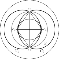
Figure 3. The case of two circles

Thus, the case of two congruent circles can be excluded and we may assume that the eigenvalues of $M_{0}$ and $M_{1}$ are ordered according to

(11) $$1<\nu_{0,1}<\nu_{1,1}\leq\nu_{1,2}<\nu_{0,2}.$$

Now we compute the derivative of the area function (6) with respect to $\lambda$. For that purpose, we assume that $C_{0}$ is given by the normal form (4) and $C_{1}$ is obtained from an ellipse in this normal form by a hyperbolic rotation, that is,

(12) $$M_{0}=\operatorname{diag}(-1,\nu_{0,1},\nu_{0,2}),\quad M_{1}=(Q^{-1})^{\mathrm{T}}\cdot\operatorname{diag}(-1,\nu_{1,1},\nu_{1,2})\cdot Q^{-1}$$

with the hyperbolic rotation matrix

(13) $$\begin{gathered}Q=\begin{pmatrix}q_{0}^{2}+q_{1}^{2}+q_{2}^{2}+q_{3}^{2}&2(q_{0}q_{3}+q_{1}q_{2})&2(q_{1}q_{3}-q_{0}q_{2})\\ 2(q_{0}q_{3}-q_{1}q_{2})&q_{0}^{2}-q_{1}^{2}-q_{2}^{2}+q_{3}^{2}&2(q_{0}q_{1}-q_{2}q_{3})\\ 2(-q_{0}q_{2}-q_{1}q_{3})&2(-q_{0}q_{1}-q_{2}q_{3})&q_{0}^{2}-q_{1}^{2}+q_{2}^{2}-q_{3}^{2}\end{pmatrix},\\ q_{0}^{2}+q_{1}^{2}-q_{2}^{2}-q_{3}^{2}=1.\end{gathered}$$

Up to the irrelevant sign of $q_{1}$ and an index shift, this is precisely Equation (5) of [13]. The rotation angle $-2\xi$ is given by $q_{0}=\cos\xi$, the axis direction is $(-q_{1},q_{2},q_{3})^{\mathrm{T}}$. A hyperbolic half-turn is obtained by substituting $q_{0}=0$ into (13). In this case, $Q\cdot Q$ indeed equals the unit matrix $\operatorname{diag}(1,1,1)$.

The matrix $M_{\lambda}$ to $C_{\lambda}$ is computed according to Definition 6. Its ordered eigenvalues $(\nu_{0},\nu_{1},\nu_{2})$ are functions of $\lambda$. In the vicinity of $\lambda=0$ we have $\nu_{0}(\lambda)>0$ and $1<\nu_{1}(\lambda)<\nu_{2}(\lambda)$. These eigenvalues are implicitly defined as roots of the characteristic polynomial $P(\lambda,\nu(\lambda))=\det(M_{\lambda}-\nu I)$ of $M_{\lambda}$ where $I$ is the matrix defined in (3). For $\lambda=0$ we know the values of these roots:

$$\nu_{0}(0)=1,\quad\nu_{1}(0)=\nu_{0,1},\quad\nu_{2}(0)=\nu_{0,2}.$$

By implicit derivation we have

$$\mathinner{\dfrac{\operatorname{d\!}{}\nu_{i}}{\operatorname{d\!}{\lambda}}}(0)=-\frac{\dfrac{\partial{}P}{\partial{\lambda}}(0,\nu_{i}(0))}{\dfrac{\partial{}P}{\partial{\nu}}(0,\nu_{i}(0))},\quad i=0,1,2.$$

Furthermore, we can compute the partial derivatives

$$\mathinner{\dfrac{\partial{}\operatorname{area}(\nu_{0},\nu_{1},\nu_{2})}{\partial{\nu_{i}}}},\quad i=0,1,2$$

of (6). Using the chain rule

$$\mathinner{\dfrac{\partial{}\operatorname{area}(C_{\lambda})}{\partial{\lambda}}}\Big{|}_{\lambda=0}=\mathinner{\dfrac{\partial{}\operatorname{area}}{\partial{\nu_{0}}}}\mathinner{\dfrac{\partial{}\nu_{0}}{\partial{\lambda}}}\Big{|}_{\lambda=0}+\mathinner{\dfrac{\partial{}\operatorname{area}}{\partial{\nu_{1}}}}\mathinner{\dfrac{\partial{}\nu_{1}}{\partial{\lambda}}}\Big{|}_{\lambda=0}+\mathinner{\dfrac{\partial{}\operatorname{area}}{\partial{\nu_{2}}}}\mathinner{\dfrac{\partial{}\nu_{2}}{\partial{\lambda}}}\Big{|}_{\lambda=0},$$

we find

(14) $$\mathinner{\dfrac{\partial{}\operatorname{area}(C_{\lambda})}{\partial{\lambda}}}\Big{|}_{\lambda=0}=-\frac{1}{2}\int_{-\pi}^{\pi}\frac{D}{N}\operatorname{d\!}\varphi$$

where

$$D=\mbox{} ((q_{1,2}^{2}\nu_{1,2}+q_{1,3}^{2}\nu_{1,2}-q_{1,1}^{2})\nu_{0,1}+q_{2,2}^{2}\nu_{1,1}+q_{2,3}^{2}\nu_{1,2}-q_{2,1}^{2})\sin^{2}\varphi+$$

$$((q_{1,2}^{2}\nu_{1,1}+q_{1,3}^{2}\nu_{1,2}-q_{1,1}^{2})\nu_{0,2}+q_{3,2}^{2}\nu_{1,1}+q_{3,3}^{2}\nu_{1,2}-q_{3,1}^{2})\cos^{2}\varphi,$$

$$N=\mbox{} (\nu_{0,1}\sin^{2}\varphi+\nu_{0,2}\cos^{2}\varphi-1)^{3/2}(\nu_{0,1}\sin^{2}\varphi+\nu_{0,2}\cos^{2}\varphi)^{1/2}$$

and $q_{i,j}$ are the entries of the matrix (13). It will be convenient to write (14) in terms of the first and second complete elliptic integrals

(15) $$K(z)=\int_{0}^{1}\frac{1}{\sqrt{1-t^{2}}\sqrt{1-z^{2}t^{2}}}\operatorname{d\!}t\quad\text{and}\quad E(z)=\int_{0}^{1}\frac{\sqrt{1-z^{2}t^{2}}}{\sqrt{1-t^{2}}}\operatorname{d\!}t.$$

Since we will evaluate them only at

$$f=\sqrt{\frac{\nu_{0,2}-\nu_{0,1}}{(\nu_{0,2}-1)\nu_{0,1}}},$$

we use the abbreviations $\bar{E}\mathrel{\mathop{\mathchar 58\relax}}=E(f)$ and $\bar{K}\mathrel{\mathop{\mathchar 58\relax}}=K(f)$. By (11), $f$ is always real and between 0 and 1. Substituting

$$\varphi=\arcsin\sqrt{\frac{\nu_{0,2}-x}{\nu_{0,2}-\nu_{0,1}}},$$

and noting that $2(\nu_{0,2}-x)(x-\nu_{0,1})=2(\nu_{0,1}-\nu_{0,2})\cos\varphi\sin\varphi$ we can express the derivative of the area function in terms of $\bar{E}$ and $\bar{K}$:

(16) $$\mathinner{\dfrac{\partial{}\operatorname{area}(C_{\lambda})}{\partial{\lambda}}}\Big{|}_{\lambda=0}=\frac{2}{\sqrt{(\nu_{0,2}-1)\nu_{0,1}}(\nu_{0,2}-\nu_{0,1})(\nu_{0,1}-1)}\\ (\mathrm{A}(q_{1,2}^{2}\nu_{1,1}+q_{1,3}^{2}\nu_{1,2}-q_{1,1}^{2})+\mathrm{B}(q_{2,2}^{2}\nu_{1,1}+q_{2,3}^{2}\nu_{1,2}-q_{2,1}^{2})+\Gamma(q_{3,2}^{2}\nu_{1,1}+q_{3,3}^{2}\nu_{1,2}-q_{3,1}^{2}))$$

where

(17) $$\begin{gathered}\mathrm{A}=-\nu_{0,1}(\nu_{0,2}-\nu_{0,1})\bar{E},\quad\mathrm{B}=\nu_{0,2}(\nu_{0,1}-1)\bar{K}-\nu_{0,1}(\nu_{0,2}-1)\bar{E},\\ \Gamma=\nu_{0,1}(\nu_{0,1}-1)(\bar{E}-\bar{K}).\end{gathered}$$

Having computed (16), the preparatory work for the final (big) step in the proof of Theorem 1 is completed. We formulate the last step as a lemma:

Lemma 7 (Hyperbolic Half-Turn Lemma).

Consider three ellipses $C_{0}$, $C_{1}$, $C^{\star}_{1}$ of equal area. Assume that

• $C_{0}$ and $C^{\star}_{1}$ are concentric,

• $C_{1}$ is obtained from $C^{\star}_{1}$ by a half-turn,

• the eigenvalues $\nu_{i,1}$, $\nu_{i,2}$ of the normalized matrix $M_{i}$ to $C_{i}$ ($i=0,1$) satisfy  (11), and

• $H(\nu_{i,1},\nu_{i,2})\leq 0$ where $H$ is defined in Equation (1).

Then the area of $C_{\lambda}=(1-\lambda)C_{0}+\lambda C_{1}$ is smaller than the area of $C^{\star}_{\lambda}=(1-\lambda)C_{0}+\lambda C^{\star}$, at least in the vicinity of $\lambda=0$.

In order to proof Lemma 7, we compare the derivatives of the areas of $C_{\lambda}$ and $C^{\star}_{\lambda}$ with respect to $\lambda$ at $\lambda=0$. The ellipse $C^{\star}_{1}$ can be obtained from an ellipse in normal form (4) by a rotation about $(1,0,0)^{\mathrm{T}}$ through $\zeta$. We can compute the matrix $M_{1}$ as in (12) by substituting

$$q_{0}=\cos\tfrac{\zeta}{2},\quad q_{1}=-\sin\tfrac{\zeta}{2},\quad q_{2}=q_{3}=0$$

into the matrix (13). Plugging this into Equation (16) yields

$$\frac{1}{2}\mathinner{\dfrac{\partial{}\operatorname{area}(C^{\star}_{\lambda})}{\partial{\lambda}}}\Big{|}_{\lambda=0}=\frac{D^{\star}_{1}}{N^{\star}_{1}}$$

where

$$D^{\star}_{1} =-\mathrm{A}+(\mathrm{B}\cos^{2}\zeta+\Gamma\sin^{2}\zeta)\nu_{1,1}+(\mathrm{B}\sin^{2}\zeta+\Gamma\cos^{2}\zeta)\nu_{1,2},$$

$$N^{\star}_{1} =\sqrt{(\nu_{0,2}-1)\nu_{0,1}}(\nu_{0,2}-\nu_{0,1})(\nu_{0,1}-1),$$

and $\mathrm{A}$, $\mathrm{B}$, $\Gamma$ are as in (17).

The ellipse $C_{1}$ is obtained by a half-turn from $C^{\star}_{1}$ about the rotation axis defined by the unit vector $r=(r_{1},r_{2},r_{3})^{\mathrm{T}}$. The matrix $Q$ in (13) is the product of the rotation matrix about $(1,0,0)^{\mathrm{T}}$ through $\zeta$ and a half-turn rotation matrix about the unit vector $r$. The later is obtained by substituting

$$q_{0}=0,\quad q_{1}=-r_{1},\quad q_{2}=r_{2},\quad q_{3}=r_{3}$$

into Equation (13). Plugging the entries of the product matrix into (16) yields

$$\frac{1}{2}\mathinner{\dfrac{\partial{}\operatorname{area}(C_{1})}{\partial{\lambda}}}\Big{|}_{\lambda=0}\equiv\frac{D_{1}}{N_{1}}\mod(r_{1}^{2}-r_{2}^{2}-r_{3}^{2}-1)$$

where $N_{1}=N_{1}^{\star}$ and

$$D_{1}= \phantom{\mbox{}+\mbox{}}4r_{2}r_{3}((2\mathrm{A}+\mathrm{B}+\Gamma)r_{1}^{2}+(\mathrm{B}-\Gamma)r_{2}^{2}-(\mathrm{B}-\Gamma)r_{3}^{2})(\nu_{1,1}-\nu_{1,2})\sin\zeta\cos\zeta$$

$$+(4(\mathrm{A}+\mathrm{B})r_{1}^{2}r_{2}^{2}-4(\mathrm{A}+\Gamma)r_{1}^{2}r_{3}^{2}-8(\mathrm{B}-\Gamma)r_{2}^{2}r_{3}^{2}+\mathrm{B}-\Gamma)(\nu_{1,1}-\nu_{1,2})\cos^{2}\zeta$$

$$+4(\mathrm{A}+\mathrm{B})r_{1}^{2}r_{2}^{2}(\nu_{1,2}-1)+4(\mathrm{A}+\Gamma)r_{1}^{2}r_{3}^{2}(\nu_{1,1}-1)$$

$$+4(\mathrm{B}-\Gamma)r_{2}^{2}r_{3}^{2}(\nu_{1,1}-\nu_{1,2})+\Gamma\nu_{1,1}+\mathrm{B}\nu_{1,2}-\mathrm{A}.$$

Now we are going to prove the inequality $D_{1}-D^{\star}_{1}<0$ for $\zeta\in[0,\frac{\pi}{2}]$. We substitute $\zeta=2\arctan t$ into its left-hand side and obtain a rational expression in $t$. Clearing the positive denominator $(1+t^{2})^{2}$, we are left with a polynomial $P(t)$ of degree four whose negativity on $[0,1]$ has to be shown. To do this, we write $P(t)$ with respect to the Bernstein basis as

(18) $$P(t)=\sum_{i=0}^{4}p_{i}B^{4}_{i}(t)\quad\text{where}\quad B^{4}_{i}(t)=\binom{4}{i}(1-t)^{4-i}t^{i}$$

and show non-positivity of the coefficients $p_{1}$, $p_{2}$, $p_{3}$ and negativity of the coefficients $p_{0}$ and $p_{4}$. After a straightforward basis transformation and reducing modulo $r_{1}^{2}-r_{2}^{2}-r_{3}^{2}-1$ we find

$$p_{0}=4((\nu_{1,1}-1)(\mathrm{A}+\mathrm{B})r_{1}^{2}r_{2}^{2}+(\nu_{1,2}-1)(\mathrm{A}+\Gamma)r_{1}^{2}r_{3}^{2}+(\nu_{1,2}-\nu_{1,1})(\mathrm{B}-\Gamma)r_{2}^{2}r_{3}^{2}),$$

$$p_{1}=4((\nu_{1,1}-1)(\mathrm{A}+\mathrm{B})r_{1}^{2}r_{2}^{2}+(\nu_{1,2}-1)(\mathrm{A}+\Gamma)r_{1}^{2}r_{3}^{2}+(\nu_{1,2}-\nu_{1,1})(\mathrm{B}-\Gamma)r_{2}^{2}r_{3}^{2})\\ +2r_{2}r_{3}(\nu_{1,2}-\nu_{1,1})(-(2\mathrm{A}+\mathrm{B}+\Gamma)r_{1}^{2}-(\mathrm{B}-\Gamma)r_{2}^{2}+(\mathrm{B}-\Gamma)r_{3}^{2}),$$

$$3p_{2}=8(\nu_{1,1}+\nu_{1,2}-2)((\mathrm{A}+\mathrm{B})r_{1}^{2}r_{2}^{2}+(\mathrm{A}+\Gamma)r_{1}^{2}r_{3}^{2})\\ +12r_{2}r_{3}(\nu_{1,2}-\nu_{1,1})(-(2\mathrm{A}+\mathrm{B}+\Gamma)r_{1}^{2}-(\mathrm{B}-\Gamma)r_{2}^{2}+(\mathrm{B}-\Gamma)r_{3}^{2}),$$

$$p_{3}=8((\nu_{1,2}-1)(\mathrm{A}+\mathrm{B})r_{1}^{2}r_{2}^{2}+(\nu_{1,1}-1)(\mathrm{A}+\Gamma)r_{1}^{2}r_{3}^{2}-(\nu_{1,2}-\nu_{1,1})(\mathrm{B}-\Gamma)r_{2}^{2}r_{3}^{2})\\ +4r_{2}r_{3}(\nu_{1,2}-\nu_{1,1})(-(2\mathrm{A}+\mathrm{B}+\Gamma)r_{1}^{2}-(\mathrm{B}-\Gamma)r_{2}^{2}+(\mathrm{B}-\Gamma)r_{3}^{2}),$$

$$p_{4}=16((\nu_{1,2}-1)(\mathrm{A}+\mathrm{B})r_{1}^{2}r_{2}^{2}+(\nu_{1,1}-1)(\mathrm{A}+\Gamma)r_{1}^{2}r_{3}^{2}-(\nu_{1,2}-\nu_{1,1})(\mathrm{B}-\Gamma)r_{2}^{2}r_{3}^{2}).$$

Recall now Equation (11) ($1<\nu_{0,1}<\nu_{1,1}\leq\nu_{1,2}<\nu_{0,2}$) and $r_{1}^{2}-r_{2}^{2}-r_{3}^{2}=1$ and observe that

• $\mathrm{A}<\mathrm{B}<\Gamma$; this is proved in Lemma 9 and Lemma 10 in the appendix.

• $\Gamma<0$; this follows from $\bar{E}<\bar{K}$ and $\nu_{0,1}>1$.

Under these conditions, the negativity of $p_{0}$ is clear except when $r_{2}=r_{3}=0$. But this is the concentric case $C_{1}=C^{\star}_{1}$ and need not be considered. The non-positivity of the coefficients $p_{1}$, $p_{2}$, $p_{3}$, and the negativity of $p_{4}$ is shown in Lemmas 12 and 13 below. This concludes the proof of the Half-Turn Lemma and, thus, also the proof of Theorem 1.

Example 8.

We use the prerequisites of Theorem 1 on the radii $r$ and $R$ in Lemma 12. But one might wonder whether the Half-Turn Lemma remains true without these assumptions. The answer to this question is negative. We can provide and example, where the polynomial $P(t)$ attains positive values on $(0,1)$.

Substituting $r_{1}^{2}=r_{2}^{2}+r_{3}^{2}+1$, the coefficient $p_{1}$ can be written as

$$p_{1} =\nu_{1,2}(4r_{2}^{2}r_{3}(\mathrm{A}+\mathrm{B})(r_{3}-r_{2})+4r_{3}^{2}(\mathrm{A}+\Gamma)(r_{3}^{2}-r_{2}r_{3}+1)-2(2\mathrm{A}+\mathrm{B}+\Gamma)r_{2}r_{3})$$

$$+\nu_{1,1}(4(\mathrm{A}+\mathrm{B})r_{2}^{2}(r_{2}^{2}+r_{2}r_{3}+1)+4(\mathrm{A}+\Gamma)r_{2}r_{3}^{2}(r_{2}+r_{3})+2(2\mathrm{A}+\mathrm{B}+\Gamma)r_{2}r_{3})$$

$$-4(1+r_{2}^{2}+r_{3}^{2})(r_{2}^{2}(\mathrm{A}+\mathrm{B})+r_{3}^{2}(\mathrm{A}+\Gamma)).$$

Assuming $r_{2}$, $r_{3}>0$ we see that

• the coefficient of $\nu_{1,1}$ is always negative and

• it is possible to choose $\nu_{0,1}$, $\nu_{0,2}$, $r_{2}$, and $r_{3}$ so that the coefficient of $\nu_{1,2}$ is positive.

Consequently $p_{1}$ can be made positive for large $\nu_{1,2}$. The choice

$$\nu_{0,1}=\nu_{1,1}=1.1,\quad\nu_{0,2}=\nu_{1,2}=90,\quad r_{2}=0.9\cos(0.3),\quad r_{3}=0.9\sin(0.3),$$

accomplishes this and even makes $P(t)$ attain positive values for $t\in(0,1)$ (the zeros are $t\approx 0.1272$ and $t\approx 0.1389$). Note that this does not imply

$$\dfrac{\partial{}\operatorname{area}(C_{\lambda})}{\partial{\lambda}}\Big{|}_{\lambda=0}>0$$

and, thus, constitutes no counter-example to the statement that the area of $C_{\lambda}$ is smaller than the area of $C_{0}$ and $C_{1}$. We are not aware of such a counter-example.

6. Conclusion and future research

We proved uniqueness results for minimal enclosing ellipses in the hyperbolic plane. The general result (Theorem 1) involves rather cumbersome but straightforward calculations. The differences to the elliptic case are mainly in the final estimates for the coefficients of the polynomial $P(t)$ in (18) and can be found in the appendix.

It is apparent that Theorem 1 leaves room for improvements. Pushing back the frontier dictated by the inequality (1) in Theorem 1 would be nice. Substantial steps towards answering the question whether the minimal area ellipse to all compact and full-dimensional sets $F$ in the hyperbolic plane is unique or not would be great.

Note that there is a subtle difference to the situation in the elliptic plane. In [18], we presented an example from which we inferred that uniqueness in the elliptic plane cannot be proved by means of our construction of in-between conics. In the hyperbolic plane, we are not aware of such a configuration. Example 8 only shows that the estimate of the derivative of the area function is insufficient. Thus, there is a certain hope that a general uniqueness result can be proved by means of our construction.

Since uniqueness or non-uniqueness of minimal enclosing ellipses in the elliptic and hyperbolic plane remains a difficult topic, one might try to aim at a weaker result and consider only “typical” (in the sense of Baire categories, see [6, 7]) convex sets $\overline{F}$.

We would also like to mention that [18] and this article are the only results on extremal quadrics in non-Euclidean geometries that we are aware of. We can conceive numerous possibilities for generalizations. They pertain to the dimension of the surrounding space, the type of the quadric and enclosed set (for example minimal enclosing hyperbolas to line sets as in [15]) the measure for the quadric’s size (volume, surface area etc.), and the replacement of “minimal enclosing” by “maximal inscribed” quadrics.

The attentive reader will have noticed that our method of proving Theorem 1 can be adapted to these generalizations. Having defined an “in-between” quadric $Q_{\lambda}$ by means of a suitable matrix convex combination, it might be infeasible to compute the size $Q_{\lambda}$ in a form that allows further processing. But, provided the size function’s derivatives with respect to the matrix eigenvalues can be computed, it is, at least in principle, possible to obtain an explicit formula for the derivative of the size of $Q_{\lambda}$ for $\lambda=0$. Its negativity has to be shown so that the uniqueness problem is made accessible to numerous tools and techniques related to inequalities.

In the Euclidean setting, the mere uniqueness result is less important than John’s characterization of it via his famous decomposition of the identity. The original reference is the old paper [10]. But, following [1], many contemporary authors considered this topic [9, 8, 12, 2, 5]. Elliptic and hyperbolic versions of John’s characterization seem to be a worthy topic of future research.

Appendix. Proofs of auxiliary results

Lemma 9.

For $\mathrm{A}$ and $\mathrm{B}$ as in (17) we have $\mathrm{A}<\mathrm{B}$.

Proof.

We show that $A-B<0$. By (17) we have

$$\mathrm{A}-\mathrm{B}=(\nu_{0,1}-1)(\nu_{0,1}\bar{E}-\nu_{0,2}\bar{K}).$$

This is negative because of $\bar{E}<\bar{K}$ and $1<\nu_{0,1}<\nu_{0,2}$. ∎

Lemma 10.

For $\mathrm{B}$ and $\Gamma$ as in (17) we have $\mathrm{B}<\Gamma$.

Proof.

We let $\Delta=\mathrm{B}-\Gamma$ and view $\Delta$ as a function of $\nu_{0,1}$ and $\nu_{0,2}$. Its negativity for $1<\nu_{0,1}<\nu_{0,2}$ follows from three facts:

• $\Delta=0$ for $\nu_{0,1}=\nu_{0,2}$ (this is obvious because in this case we have $\bar{E}=\bar{K}$),

• $\dfrac{\partial{}\Delta}{\partial{\nu_{0,2}}}=0$ for $\nu_{0,1}=\nu_{0,2}$, and

• $\Delta$ is concave in $\nu_{0,2}$ for $1<\nu_{0,1}<\nu_{0,2}$.

We compute the first partial derivative of $\Delta$ with respect to $\nu_{0,2}$:

$$\dfrac{\partial{}\Delta}{\partial{\nu_{0,2}}}=\frac{(2\nu_{0,2}(1-\nu_{0,2})+\nu_{0,1}-1)\nu_{0,1}\bar{E}}{2\nu_{0,2}(\nu_{0,2}-1)}+\frac{(2\nu_{0,2}-1)(\nu_{0,1}-1)\bar{K}}{2(\nu_{0,2}-1)}.$$

It vanishes for $\nu_{0,1}=\nu_{0,2}$. The second partial derivative of $\Delta$ with respect to $\nu_{0,2}$ equals

$$\mathinner{\dfrac{\partial{{}^{2}}\Delta}{\partial{\nu_{0,2}^{2}}}}=\frac{(\nu_{0,1}-1)}{4\nu_{0,2}^{2}(\nu_{0,2}-1)^{2}}J_{1}\quad\text{where}\quad J_{1}=\nu_{0,2}(\nu_{0,1}-1)\bar{K}-\nu_{0,1}(5\nu_{0,2}-2)\bar{E}.$$

We have to show that it is negative. The factor before $J_{1}$ is positive. To see the negativity of $J_{1}$ itself we write it in the integral form (see (15))

$$J_{1}=\int_{0}^{1}\frac{J_{2}}{\sqrt{1-t^{2}}\sqrt{1-f^{2}t^{2}}}\operatorname{d\!}t,$$

where

$$J_{2}=\nu_{0,2}(\nu_{0,1}-1)-\nu_{0,1}(5\nu_{0,2}-2)\Bigl{(}1-t^{2}\frac{\nu_{0,2}-\nu_{0,1}}{\nu_{0,1}(\nu_{0,2}-1)}\Bigr{)}.$$

The term $J_{2}$ is linear in $t^{2}$. For $t=0$ it equals $2\nu_{0,1}(1-2\nu_{0,2})-\nu_{0,2}<0$ and for $t=1$ it equals $-\nu_{0,2}(\nu_{0,1}-1)(4\nu_{0,2}-1)/(\nu_{0,2}-1)<0$. Thus, $J_{2}<0$ for $t\in[0,1]$. This implies $J_{1}<0$ and we see that $\Delta$ is indeed concave for $1<\nu_{0,1}<\nu_{0,2}$. ∎

We will deduce non-positivity of the Bernstein coefficients $p_{1}$, …, $p_{3}$ from the inequality (1) and the additional inequalities

(19) $$h_{1}(\nu_{1},\nu_{2}) \mathrel{\mathop{\mathchar 58\relax}}=\nu_{2}-5\nu_{1}+4\leq 0,$$

(20) $$h_{2}(\nu_{1},\nu_{2}) \mathrel{\mathop{\mathchar 58\relax}}=-5\nu_{1}^{2}+\nu_{1}\nu_{2}+\nu_{1}+\nu_{2}+2\leq 0,$$

(21) $$h_{3}(\nu_{1},\nu_{2}) \mathrel{\mathop{\mathchar 58\relax}}=\nu_{2}^{2}-5\nu_{1}\nu_{2}-2\nu_{1}+4\nu_{2}+2\leq 0,$$

(22) $$h_{4}(\nu_{1},\nu_{2}) \mathrel{\mathop{\mathchar 58\relax}}=5\nu_{2}^{2}-13\nu_{1}\nu_{2}-2\nu_{1}+6\nu_{2}+4\leq 0,$$

(23) $$h_{5}(\nu_{1},\nu_{2}) \mathrel{\mathop{\mathchar 58\relax}}=-5\nu_{1}^{2}+\nu_{1}\nu_{2}-\nu_{1}+3\nu_{2}+2\leq 0,$$

(24) $$h_{6}(\nu_{1},\nu_{2}) \mathrel{\mathop{\mathchar 58\relax}}=\nu_{2}^{2}-5\nu_{1}\nu_{2}+2\nu_{2}+2\leq 0,$$

which are all simple consequences of (1). We state this in Lemma 11, below.

The assumptions of Theorem 1 guarantee that these inequalities are fulfilled for $\nu_{1}=\nu_{0,1}$, $\nu_{2}=\nu_{0,2}$. Thus, we only have to show that the inequalities are satisfied on the set

$$U\mathrel{\mathop{\mathchar 58\relax}}=\{(\nu_{1},\nu_{2})\mid 1<\nu_{1}<\nu_{2}\}.$$

Lemma 11.

(a) If a point $(\nu_{1},\nu_{2})\in U$ satisfies the inequality (1), it also satisfies the inequalities (19)–(24).

(b) If a point $(\nu_{1}^{\star},\nu_{2}^{\star})$ satisfies the inequalities (1), and (19)–(24), the same is true for all points $(\nu_{1},\nu_{2})\in U$ with $\nu_{1}\geq\nu_{1}^{\star}$ and $\nu_{2}\leq\nu_{2}^{\star}$.

Proof.

It is an elementary exercise to verify that the curves defined by the implicit equations $H$ and $h_{j}$ over the closure of $U$ are the graphs of strictly monotone increasing functions of $F(\nu_{1})$ and $f_{j}(\nu_{1})$

$$F,f_{j}\colon[1,\infty)\to[1,\infty),$$

for $j\in\{1,\ldots,6\}$. This implies assertion (b).

The functions $f_{j}-F$ are strictly monotone increasing as well. This and the observation $F(1)=f_{j}(1)=1$ implies assertion (a). ∎

Figure 1 displays the hyperbolas $H(\nu_{1},\nu_{2})=0$ and, as an example, $h_{2}(\nu_{1},\nu_{2})=0$ together with the line $\nu_{1}=\nu_{2}$. The remaining curves are depicted in light-gray. The region $U$ is dotted.

Lemma 12.

The coefficients $p_{1}$, $p_{2}$, and $p_{3}$ are not positive.

Proof.

We substitute $r_{1}^{2}=1+r_{2}^{2}+r_{3}^{2}$ into $p_{1}$ and observe that $p_{1}=0$ and $\dfrac{\partial{}p_{1}}{\partial{r_{2}}}=0$ if $r_{2}=r_{3}=0$. The lemma’s claim holds true if we can show that the $r_{2}$-parameter lines of $p_{1}$, viewed as a function of $r_{2}$ and $r_{3}$, are strictly concave, that is,

(25) $$\mathinner{\dfrac{\partial{{}^{2}}p_{1}}{\partial{r_{2}^{2}}}}=8(\mathrm{A}+\mathrm{B})(\nu_{1,1}-1)(6r_{2}^{2}+1)\\ +8((\mathrm{A}+\mathrm{B})\nu_{1,2}+(\mathrm{A}+\Gamma)\nu_{1,1}-(2\mathrm{A}+\mathrm{B}+\Gamma))r_{3}^{2}-24(\nu_{1,2}-\nu_{1,1})(\mathrm{A}+\mathrm{B})r_{2}r_{3}<0.$$

The coefficient of $r_{2}r_{3}$ is positive, the remaining terms are negative. By the inequality of arithmetic and geometric means we have $r_{2}r_{3}\leq(r_{2}^{2}+r_{3}^{2})/2$. We insert this into (25) to obtain

(26) $$\mathinner{\dfrac{\partial{{}^{2}}p_{1}}{\partial{r_{2}^{2}}}}\leq 4(\mathrm{A}+\mathrm{B})(3(-\nu_{1,2}+5\nu_{1,1}-4)r_{2}^{2}+2(\nu_{1,1}-1))\\ +4(-(\mathrm{A}+\mathrm{B})\nu_{1,2}+(5\mathrm{A}+3\mathrm{B}+2\Gamma)\nu_{1,1}-2(2\mathrm{A}+\mathrm{B}+\Gamma))r_{3}^{2}<0.$$

The first term is negative if $\nu_{1,2}-5\nu_{1,1}+4\leq 0$. This is implied by $\nu_{0,2}-5\nu_{0,1}+4\leq 0$ and thus follows from (19). In the second term the coefficient of $r_{3}^{2}$ needs closer investigation. We want to show its negativity. By (11) we have

(27) $$(5\mathrm{A}+3\mathrm{B}+2\Gamma)\nu_{1,1}-(\mathrm{A}+\mathrm{B})\nu_{1,2}-2(2\mathrm{A}+\mathrm{B}+\Gamma)\leq\\ (5\mathrm{A}+3\mathrm{B}+2\Gamma)\nu_{0,1}-(\mathrm{A}+\mathrm{B})\nu_{0,2}-2(2\mathrm{A}+\mathrm{B}+\Gamma).$$

Using (15) and (17), we write the term on the right in its integral form:

(28) $$(5\mathrm{A}+3\mathrm{B}+2\Gamma)\nu_{0,1}-(\mathrm{A}+\mathrm{B})\nu_{0,2}-2(2\mathrm{A}+\mathrm{B}+\Gamma)\\ =(\nu_{0,2}-\nu_{0,1})\int_{0}^{1}\frac{J_{3}}{\sqrt{1-t^{2}}\sqrt{1-f^{2}t^{2}}}$$

where

$$J_{3}=-\frac{\nu_{0,2}-\nu_{0,1}}{\nu_{0,2}-1}(2\nu_{0,2}-7\nu_{0,1}+5)t^{2}+\nu_{0,2}(\nu_{0,1}+1)+\nu_{0,1}(1-5\nu_{0,1})+2.$$

We see that $J_{3}$ is linear in $t^{2}$. For $t=0$ and $t=1$ it attains the respective values

(29) $$J_{3}\big{|}_{t=0} =-5\nu_{0,1}^{2}+\nu_{0,1}\nu_{0,2}+\nu_{0,1}+\nu_{0,2}+2,$$

(30) $$J_{3}\big{|}_{t=1} =\frac{\nu_{0,1}-1}{\nu_{0,2}-1}(\nu_{0,2}^{2}-5\nu_{0,1}\nu_{0,2}-2\nu_{0,1}+4\nu_{0,2}+2).$$

The right-hand side of (29) is not positive by (20). The right-hand side of (30) is not positive by (21). We conclude that the integrand $J_{3}$ is not positive for $t\in[0,1]$ and the same is true for $\dfrac{\partial{{}^{2}}p_{1}}{\partial{r_{2}^{2}}}$. Hence, the coefficient $p_{1}$ as a function of $r_{2}$ is concave with the maximum, $p_{1}=0$ attained at $r_{2}=r_{3}=0$. Thus, $p_{1}$ is not positive.

The proofs of non-positivity of $p_{2}$ and $p_{3}$ run along exactly the same lines. We only provide the relevant formulas and reduce the explanatory text between them to a minimum. Equations (25) and (26) become

$$3\mathinner{\dfrac{\partial{{}^{2}}p_{2}}{\partial{r_{2}^{2}}}} =16(\mathrm{A}+\mathrm{B})(\nu_{1,2}+\nu_{1,1}-2)(6r_{2}^{2}+1)+$$

$$\qquad 16(2\mathrm{A}+\mathrm{B}+\Gamma)(\nu_{1,2}+\nu_{1,1}-2)r_{3}^{2}-144(\mathrm{A}+\mathrm{B})(\nu_{1,2}-\nu_{1,1})r_{2}r_{3}$$

$$\leq 8(\mathrm{A}+\mathrm{B})(3(\nu_{1,2}+7\nu_{1,1}-8)r_{2}^{2}+2(\nu_{1,2}+\nu_{1,1}-2))+$$

$$\qquad 8(-(5\mathrm{A}+7\mathrm{B}-2\Gamma)\nu_{1,2}+(13\mathrm{A}+11\mathrm{B}+2\Gamma)\nu_{1,1}-4(2\mathrm{A}+\mathrm{B}+\Gamma))r_{3}^{2}.$$

Instead of (27) and (28) we have

$$\begin{gathered}-(5\mathrm{A}+7\mathrm{B}-2\Gamma)\nu_{1,2}+(13\mathrm{A}+11\mathrm{B}+2\Gamma)\nu_{1,1}-4(2\mathrm{A}+\mathrm{B}+\Gamma)\leq\\ -(5\mathrm{A}+7\mathrm{B}-2\Gamma)\nu_{0,2}+(13\mathrm{A}+11\mathrm{B}+2\Gamma)\nu_{0,1}-4(2\mathrm{A}+\mathrm{B}+\Gamma)=\\ (\nu_{0,2}-\nu_{0,1})\int_{0}^{1}\frac{J_{4}}{\sqrt{1-t^{2}}\sqrt{1-f^{2}t^{2}}}\operatorname{d\!}t\end{gathered}$$

where

$$J_{4}=-\frac{\nu_{0,2}-\nu_{0,1}}{\nu_{0,2}-1}(3(4\nu_{0,2}-5\nu_{0,1}+1)t^{2}+\nu_{0,2}(5\nu_{0,1}+7)+\nu_{0,1}(-13\nu_{0,1}-3)+4).$$

The non-positivity of $p_{2}$ follows from

$$J_{4}\big{|}_{t=0} =-13\nu_{0,1}^{2}+5\nu_{0,1}\nu_{0,2}-3\nu_{0,1}+7\nu_{0,2}+4,$$

$$J_{4}\big{|}_{t=1} =\frac{\nu_{0,1}-1}{\nu_{0,2}-1}(5\nu_{0,2}^{2}-13\nu_{0,1}\nu_{0,2}-2\nu_{0,1}+6\nu_{0,2}+4),$$

(1) and (22).

As to the coefficient $p_{3}$, Equations (25) and (26) are replaced by

$$\mathinner{\dfrac{\partial{{}^{2}}p_{3}}{\partial{r_{2}^{2}}}} =16(\nu_{1,2}-1)(\mathrm{A}+\mathrm{B})(6r_{2}^{2}+1)+$$

$$16((\mathrm{A}+\Gamma)\nu_{1,2}+(\mathrm{A}+\mathrm{B})\nu_{1,1}-(2\mathrm{A}+\mathrm{B}+\Gamma))r_{3}^{2}-48(\nu_{1,2}-\nu_{1,1})(\mathrm{A}+\mathrm{B})r_{2}r_{3}$$

$$\leq 8(\mathrm{A}+\mathrm{B})(3(3\nu_{1,2}+\nu_{1,1}-4)r_{2}^{2}+2(\nu_{1,2}-1))+$$

$$\qquad 8(-(\mathrm{A}+3\mathrm{B}-2\Gamma)\nu_{1,2}+5(\mathrm{A}+\mathrm{B})\nu_{1,1}-2(2\mathrm{A}+\mathrm{B}+\Gamma))r_{3}^{2}$$

and (27) and (28) by

$$\begin{gathered}-(\mathrm{A}+3\mathrm{B}-2\Gamma)\nu_{1,2}+5(\mathrm{A}+\mathrm{B})\nu_{1,1}-2(2\mathrm{A}+\mathrm{B}+\Gamma)\leq\\ -(\mathrm{A}+3\mathrm{B}-2\Gamma)\nu_{0,2}+5(\mathrm{A}+\mathrm{B})\nu_{0,1}-2(2\mathrm{A}+\mathrm{B}+\Gamma)=\\ (\nu_{0,2}-\nu_{0,1})\int_{0}^{1}\frac{J_{5}}{\sqrt{1-t^{2}}\sqrt{1-f^{2}t^{2}}}\end{gathered}$$

where

$$J_{5}=-\frac{\nu_{0,2}-\nu_{0,1}}{\nu_{0,2}-1}((4\nu_{0,2}-5\nu_{0,1}+1)t^{2}+\nu_{0,2}(\nu_{0,1}+3)-\nu_{0,1}(5\nu_{0,1}+1)+2).$$

The non-positivity of $p_{3}$ follows from

$$J_{5}\big{|}_{t=0} =-5\nu_{0,1}^{2}+\nu_{0,1}\nu_{0,2}-\nu_{0,1}+3\nu_{0,2}+2,$$

$$J_{5}\big{|}_{t=1} =\frac{\nu_{0,1}-1}{\nu_{0,2}-1}(\nu_{0,2}^{2}-5\nu_{0,1}\nu_{0,2}+2\nu_{0,2}+2).$$

and (23), (24). ∎

The negativity of the only remaining Bernstein coefficient can be shown directly without resorting to Lemma 11:

Lemma 13.

The coefficient $p_{4}$ is negative.

Proof.

We can write

(31) $$\frac{p_{4}}{16}=(\nu_{1,2}-1)r_{2}^{2}((\mathrm{A}+\mathrm{B})r_{1}^{2}-(\mathrm{B}-\Gamma)r_{3}^{2})+(\nu_{1,1}-1)r_{3}^{2}((\mathrm{A}+\Gamma)r_{1}^{2}+(\mathrm{B}-\Gamma)r_{2}^{2}).$$

The proof is finished, if we can show that the coefficients of $(\nu_{1,2}-1)r_{2}^{2}$ and $(\nu_{1,1}-1)r_{3}^{2}$ in (31) are negative. For the coefficient of $(\nu_{1,2}-1)r_{2}^{2}$ we argue as follows: $\mathrm{A}<\mathrm{B}<\Gamma<0$ implies $\mathrm{A}+\mathrm{B}<\mathrm{A}<\mathrm{B}<\mathrm{B}-\Gamma$ and $r_{1}^{2}-r_{2}^{2}-r_{3}^{2}=1$ implies $r_{1}^{2}>r_{3}^{2}$. Thus, $(\mathrm{A}+\mathrm{B})r_{1}^{2}-(\mathrm{B}-\Gamma)r_{3}^{2}<0$. The negativity of the coefficient of $(\nu_{1,2}-1)r_{3}^{2}$ follows from $\mathrm{A}+\Gamma<0$ and $\mathrm{B}-\Gamma<0$. ∎

References

- Ball [1992] K. M. Ball. Ellipsoids of maximal volume in convex bodies. Geom. Dedicata, 41(2):241–250, 1992.
- Bastero and Romance [2002] J. Bastero and M. Romance. John’s decomposition of the identity in the non-convex case. Positivity, 6(1):1–16, 2002.
- Callahan [2000] J. J. Callahan. The Geometry of Spacetime. An Introduction to Special and General Relativity. Springer, New York, 2000.
- Davis [1957] Ch. Davis. All convex invariant functions of Hermitian matrices. Arch. Math., 8(4):276–278, 1957.
- Gordon et al. [2004] Y. Gordon, A. E. Litvak, M. Meyer, and A. Pajor. John’s decomposition of the identity in the general case and applications. J. Differential Geom., 68(1):99–119, 2004.
- Gruber [1985] P. M. Gruber. Results of baire category type in convexity. In J. Goodmann, E. Lutwak, E. Malkewitsch, and J. Pollack, editors, Discrete Geometry and Convexity, pages 163–169. New York Academy of Sciences, 1985.
- Gruber [1993] P. M. Gruber. Baire categories in convexity. In Peter M. Gruber and Jörg Wills, editors, Handbook of convex geometry, volume B, pages 1327–1346. Elsevier, 1993.
- Gruber [2008] P. M. Gruber. Application of an idea of Voronoi to John type problems. Adv. in Math., 218(2):309–351, 2008.
- Gruber and Schuster [2005] P. M. Gruber and F. E. Schuster. An arithmetic proof of John’s ellipsoid theorem. Arch. Math., 85:82–88, 2005.
- John [1948] F. John. Studies and essays. Courant anniversary volume, chapter Extremum problems with inequalities as subsidary conditions, pages 187–204. Interscience Publ. Inc., New York, 1948.
- Lewis [1996] A. S. Lewis. Convex analysis on the Hermitian matrices. SIAM J. Optim., 6(1):164–177, 1996.
- Lutwak et al. [2005] E. Lutwak, D. Yang, and G. Zhang. John ellipsoids. Proc. London Math. Soc., 90:497–520, 2005.
- Özdemir and Ergin [2006] M. Özdemir and A. A. Ergin. Rotations with unit timelike quaternions in Minkowski 3-space. J. Geom. Phys., 56(2):322–336, 2006.
- Reynold [1993] W. F. Reynold. Hyperbolic geometry on a hyperboloid. Amer. Math. Monthly, 100(5):442–455, 1993.
- Schröcker [2007] H.-P. Schröcker. Minimal enclosing hyperbolas of line sets. Beitr. Algebra Geom., 48(2):367–381, 2007.
- Schröcker [2008] H.-P. Schröcker. Uniqueness results for minimal enclosing ellipsoids. Comput. Aided Geom. Design, 25(9):756–762, 2008.
- Weber and Schröcker [2010a] M. J. Weber and H.-P. Schröcker. Davis’ convexity theorem and extremal ellipsoids. Beitr. Algebra Geom., 51(1):263–274, 2010a.
- Weber and Schröcker [2010b] M. J. Weber and H.-P. Schröcker. Minimal area conics in the elliptic plane. Submitted for publication, 2010b. URL http://arxiv.org/abs/1008.4285.