The Feigenbaum’s $\delta$ for a high dissipative bouncing ball model

Abstract

We have studied a dissipative version of a one-dimensional Fermi accelerator model. The dynamics of the model is described in terms of a two-dimensional, nonlinear area-contracting map. The dissipation is introduced via innelastic collisions of the particle with the walls and we consider the dynamics in the regime of high dissipation. For such a regime, the model exhibits a route to chaos known as period doubling and we obtain a constant along the bifurcations so called the Feigenbaum’s number $\delta$.

I Introduction

The origin of cosmic radiation and a mechanism trough which it could acquire enormous energies has intrigued many physicists and mathematicians along the last decades. In particular, in the year of 1949 Enrico Fermi ref1 proposed a very simple model that qualitatively describes a process in which charged particles were bounced via interaction with moving magnetic fields. This heuristic idea was then later modified to encompass in a suitable model that could give quantitative results on the original Fermi’s model. After that, many different versions of the model were proposed ref2 ; ref3 ; ref4 ; ref5 ; ref6 ; ref7 ; NEW1 ; NEW2 and studied in different context and considering many approaches and modifications ref8 ; ref9 ; ref10 ; ref11 ; ref12 ; ref13 ; ref14 ; ref15 . One of them is the well known Fermi-Ulam model (FUM). Such model consists of a classical point-like particle moving between two walls in the total absence of any external field. One of the walls is considered to be fixed while the other one moves periodically in time. Despite this simplicity, the structure of the phase space is rather complex and it includes a large chaotic sea surrounding KAM islands and a set of invariant spanning curves limiting the energy of a bouncing particle. However, the introduction of innelastic collisions on this model is enough to destroy such a mixed structure and the system exhibits attractors. Depending on the initial conditions and control parameters, one can observe a chaotic attractor characterised by a positive Lyapunov exponent. By a suitable control parameter variation, the chaotic attractor might be destroyed via a crisis event ref19 ; ref20 ; add1 . After the destruction, the chaotic attractor is replaced by a chaotic transient ref20 .

In this paper, we revisit a dissipative version of the Fermi-Ulam model seeking to understand and describe the behaviour of the dynamics for the regime of high dissipation. Moreover, we investigate a phenomenon quite common observed for a large variety of dissipative and nonlinear systems known as period doubling route to chaos. This route shows a sequence of doubling bifurcations connecting regular-periodic to chaotic behaviour. The main goal of this paper is then to examine and show that the Fermi-Ulam model obey the same convergence ratio as that obtained by Feigenbaum ref21 for the dynamics of the logistic map. Such a constant value has been further called as “The Feigenbaum’s $\delta$”.

The organisation of this paper is as follows: In section II we present all the details needed for the construction of the nonlinear mapping. Our numerical results are discussed in section III and our conclusions and final remarks are drawn in section IV.

II A dissipative Fermi-Ulam model

Let us describe the model and obtain the equations of the mapping. The model we are dealing with consists of a classical point-like particle confined in and bouncing betwen two rigid walls. One of them is assumed to be fixed at the position $x=l$ and the other one moves periodically in time according to $x_{w}(t)=\varepsilon\cos(\omega t)$. Thus, the moving wall velocity is given by $v_{w}(t)=-\varepsilon\omega\sin(\omega t)$ where $\varepsilon$ denotes the amplitude of oscillation and $\omega$ is the angular frequency of the moving wall, respectively. Aditionally, the motion of the particle does not suffer influence of any external field. We assume that all the collisions with both walls are inelastic. Thus, we introduce a restitution coefficient for the fixed wall as $\alpha\in[0,1]$ while for the moving wall we consider $\beta\in[0,1]$. The completely inelastic collision happens when $\alpha=\beta=0$ and that a single collision is enough to terminate all the particle’s dynamics. On the other hand, when $\alpha=\beta=1$, corresponding to a complete elastic collision, all the results for the nondissipative case are recovered ref15 .

We describe the dynamics of the particle using a map $T$ where the dynamical variables are $(v_{n},t_{n})$ and $v_{n}$ is the velocity of the particle at the instant $t_{n}$. The index $n$ denotes the $n^{th}$ collision of the particle with the moving wall. Starting then with an initial condition $(v_{n},t_{n})$, with initial position of the particles given by $x_{p}(t)=\varepsilon\cos(\omega t_{n})$ with $v_{n}>0$, the dynamics is evolved and the map $T$ gives a new pair of $(v_{n+1},t_{n+1})$ at the $(n+1)^{th}$ collision. It is important to say that we have three control parameters, namely: $\varepsilon$, $l$ and $\omega$ and that the dynamics does not depend on all of them. Thus it is convenient to define dimensionless and more appropriated variables. Therefore, we define $\epsilon=\varepsilon/l$, $V_{n}=v_{n}/{\omega l}$ and measure the time in terms of the number of oscillations of the moving wall, consequently $\phi_{n}=\omega t_{n}$. Incorporating this set of new variables into the model, the map $T$ is written as

$$T:\left\{\begin{array}[]{ll}V_{n+1}=V_{n}^{*}-(1+\beta)\epsilon\sin(\phi_{n+1}){}{}\\ \phi_{n+1}=\phi_{n}+\Delta T_{n}~{}~{}{\rm mod(2\pi)}\\ \end{array}\right.~{},$$ (1)

where the expressions for both $V_{n}^{*}$ and $\Delta T_{n}$ depend on what kind of collision occurs. There are two different possible situations, namely: (i) multiple collisions with the moving wall and, (ii) single collision with the moving wall. Considering the first case, the expressions are $V_{n}^{*}=-\beta V_{n}$ and $\Delta T_{n}=\phi_{c}$, where $\phi_{c}$ is obtained as the smallest solution of $G(\phi_{c})=0$ with $\phi_{c}\in(0,2\pi]$. A solution for $G(\phi_{c})=0$ is equivalent to have that the position of the particle is the same as that of the moving wall at the instant of the impact. The function $G(\phi_{c})$ is given by

$$G(\phi_{c})=\epsilon\cos(\phi_{n}+\phi_{c})-\epsilon\cos(\phi_{n})-V_{n}\phi_{c}~{}.$$ (2)

If the function $G(\phi_{c})$ does not have a root in the interval $\phi_{c}\in(0,2\pi]$, we can conclude that the particle leaves the collision zone (the collision zone is defined as the interval $x\in[-\epsilon,\epsilon]$) without suffering a successive collision.

Considering now the case (ii), i.e. the case where the particle leaves the collision zone, the corresponding expressions are $V_{n}^{*}=-\alpha\beta V_{n}$ and $\Delta T_{n}=\phi_{c}+\phi_{r}+\phi_{l}$, with the auxiliary terms given by

$$\phi_{r}={{1-\epsilon\cos(\phi_{n})}\over{V_{n}}}~{}~{},~{}~{}\phi_{l}={{1-\epsilon}\over{\alpha V_{n}}}~{}.$$ (3)

Finally, the term $\phi_{c}$ is obtained as the smallest solution of $F(\phi_{c})=0$ for $\phi_{c}\in[0,2\pi)$. The expression of $F(\phi_{c})$ is given by

$$F(\phi_{c})=\epsilon\cos(\phi_{n}+\phi_{r}+\phi_{l}+\phi_{c})-\epsilon+\alpha V_{n}\phi_{c}~{}.$$ (4)

Both, Eq. (2) and Eq. (4) must be solved numerically.

After some algebra it is easy to shown that the determinant of the Jacobian Matrix for the case (i) is given by

$$det(J)=\beta^{2}\left[{{V_{n}+\epsilon\sin(\phi_{n})}\over{V_{n+1}+\epsilon\sin(\phi_{n+1})}}\right]~{},$$ (5)

while for the case (ii) we obtain

$$det(J)=\alpha^{2}\beta^{2}\left[{{V_{n}+\epsilon\sin(\phi_{n})}\over{V_{n+1}+\epsilon\sin(\phi_{n+1})}}\right]~{}.$$ (6)

We therefore can conclude based on the above result that area preservation is obtained only for the case of $\alpha=\beta=1$.

III Numerical Results

In this section we discuss some numerical results considering the case of high dissipation. We call as high dissipation the situation in which a particle loses more than $50\%$ of its energy upon colision with the moving wall. Moreover, we have considered as fixed the values of the damping coefficients $\alpha=0.85$ and $\beta=0.50$. To illustrate that the dynamics of the system exhibits doubling bifurcation cascade, it is shown in Fig. 1(a)

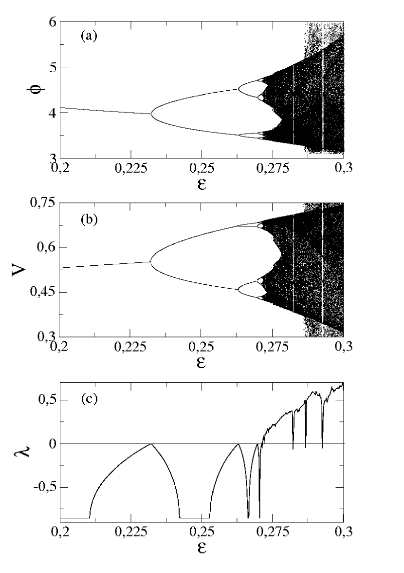
Figure 1: Bifurcation cascade for (a) $\phi$ and (b) $V$ both plotted against $\epsilon$. In (c) it is shown the Lyapunov exponent associated to (a) and (b). The damping coefficients used for the construction of the figures (a), (b) and (c) were $\alpha=0.85$ and $\beta=0.50$.

the behaviour of the asymptotic velocity plotted against the control parameter $\epsilon$, where the sequence of bifurcations is evident. A similar sequence is also observed for the asymptotic variable $\phi$, as it is shown in Fig. 1(b). Note that all the bifurcations of same period in (a) and (b) happen for the same value of the parameter $\epsilon$. At the point of bifurcations, one can also observe that the positive Lyapunov exponent shows null value, as it is shown in Fig. 1(c). It is well known that the Lyapunov exponents are important tool that can be used to classify orbits as chaotic. As discussed in ref22 , the Lyapunov exponents are defined as

$$\lambda_{j}=\lim_{n\rightarrow\infty}{1\over{n}}\ln|\Lambda_{j}|~{}~{},~{}~{}j=1,2~{}~{},$$ (7)

where $\Lambda_{j}$ are the eigenvalues of $M=\prod_{i=1}^{n}J_{i}(V_{i},\phi_{i})$ and $J_{i}$ is the Jacobian matrix evaluated over the orbit $(V_{i},\phi_{i})$. However, a direct implementation of a computational algorithm to evaluate Eq. (7) has a severe limitation to obtain $M$. Even in the limit of short $n$, the components of $M$ can assume very different orders of magnitude for chaotic orbits and periodic attractors, yielding impracticable the implementation of the algorithm. In order to avoid such problem, we note that $J$ can be written as $J=\Theta T$ where $\Theta$ is an ortoghonal matrix and $T$ is a right up triangular matrix. Thus we rewrite $M$ as $M=J_{n}J_{n-1}\ldots J_{2}\Theta_{1}\Theta_{1}^{-1}J_{1}$, where $T_{1}=\Theta_{1}^{-1}J_{1}$. A product of $J_{2}\Theta_{1}$ defines a new $J_{2}^{\prime}$. In a next step, it is easy to show that $M=J_{n}J_{n-1}\ldots J_{3}\Theta_{2}\Theta_{2}^{-1}J_{2}^{\prime}T_{1}$. The same procedure can be used to obtain $T_{2}=\Theta_{2}^{-1}J_{2}^{\prime}$ and so on. Using this procedure, the problem is reduced to evaluate the diagonal elements of $T_{i}:T_{11}^{i},T_{22}^{i}$. Finally, the Lyapunov exponents are given by

$$\lambda_{j}=\lim_{n\rightarrow\infty}{1\over{n}}\sum_{i=1}^{n}\ln|T_{jj}^{i}|~{}~{},~{}~{}j=1,2~{}~{}.$$ (8)

If at least one of the $\lambda_{j}$ is positive then the orbit is classified as chaotic. We can see in Fig. (1) (c) the behavior of the Lyapunov exponents corresponding to both Figs. (1)(a,b). It is also easy to see that when the bifurcations happen, the exponent $\lambda$ assumes the zero value at same values of the control parameter $\epsilon$ where the bifurcation hold. Another interesting observation is that the Lyapunov exponent, in some regions, assumes a constant and negative values, such behavior occurs because the eigenvalues of the Jacobian Matrix become complex numbers (imaginary numbers)).

Let us now use the points where the Lyapunov exponent assumes the null value to characterise a very interesting property of the model. As it was shown by Feigenbaum ref21 , along the bifurcations the dynamics exhibits an universal feature. It implies that all the bifurcations happen at the same rate of convergence for the bifurcation diagram changing from periodic to chaotic behavior. The procedure used to obtain the Feigenbaum value $\delta$ consists of: let $\epsilon_{1}$ represents the control parameter value at which period-1 gives birth to a period-2 orbit, $\epsilon_{2}$ is the value where period-2 changes to period-4 and so on. In general the parameter $\epsilon_{n}$ corresponds to the control parameter value at which a period-$2^{n}$ orbit is born. Thus, we write the Feigenbaum’s $\delta$ as

$$\delta_{n}={\lim_{n\gg 1}{{\epsilon_{n}-\epsilon_{n-1}}\over{\epsilon_{n+1}-\epsilon_{n}}}}.$$ (9)

The numerical value for the constant number $\delta$ obtained by Eq. (9) and considering a sufficient large values for $n$ is $\delta=4.66920161\ldots$. Considering the numerical data obtained through the Lyapunov exponents calculation, the Feigenbaum’s $\delta$ obtained for the Fermi-Ulam model is $\delta=4.64(4)$. We have considered in our simulations only the bifurcations of fourth to eighth order since the numerical results are very hard to be obtained for higher orders in the bifurcations. Our result is in a good agreement with the Feigenbaum’s universal $\delta$.

IV Conclusion

As a summary, we have studied a dissipative version of the Fermi-Ulam model. We introduce dissipation into the model through inelastic collisions with both walls. We have shown that for regimes of high dissipation, the model exhibits a sequence of doubling bifurcation cascade. For this cascade, we obtained the so called Feigenbaum’s number as $\delta=4.64(4)$.

References

- (1) E. Fermi, Phys. Rev. 75 1169 (1949).
- (2) Ulam S 1961 Proc. 4th Berkeley Symposium on Math, Statistics and Probability vol 3 (Berkeley, CA: California University Press) p 315.
- (3) A. J. Lichtenberg, M.A. Lieberman, “Regular and Chaotic Dynamics” (Appl. Math. Sci. 38, Springer Verlag, New York, (1992).
- (4) A. J. Lichtenberg, M.A. Lieberman and R. H. Cohen, Physica D 1, 291 (1980).
- (5) P. J. Holmes, J. Sound and Vibr. 84, 173 (1982).
- (6) K. Y. Tsang and M. A. Lieberman, Physica D 11, 147 (1984).
- (7) M. A. Lieberman and K. Y. Tsang, Phys. Rev. Lett. 55, 908 (1985).
- (8) J. K. L. da Silva, D. G. Ladeira, E. D. Leonel, P. V. E. McClintock, S. O. Kamphorst, Brazilian Journal of Physics 36, 700 (2006).
- (9) E. D. Leonel, D. F. M. Oliveira, R. E. de Carvalho, Physica A 386, 73 (2007).
- (10) R. M. Everson, Physica D 19, 355 (1986).
- (11) J. V. José and R. Cordery, Phys. Rev. Lett. 56, 290 (1986).
- (12) G. A. Luna-Acosta, Phys. Rev. 42, 7155 (1990).
- (13) S. T. Dembinski, A. J. Makowski and P. Peplowski, Phys. Rev. Lett. 70, 1093 (1993).
- (14) E. D. Leonel, P. V. E. McClintock and J. K. L. da Silva, Phys. Rev. Lett. 93, 014101 (2004).
- (15) E. D. Leonel and P. V. E. McClintock, J. Phys. A 38, 823 (2005).
- (16) D. G. Ladeira, J. K. L. da Silva, Phys. Rev. E 73, 026201 (2006).
- (17) E. D. Leonel, J. K. L. da Silva and S. O. Kamphorst, Physica A 331, 435 (2004).
- (18) E. D. Leonel and P. V. E. McClintock, J. Phys. A, 38, L425 (2005).
- (19) E. D. Leonel and R. Egydio de Carvalho, Phys. Lett. A, 364, 475 (2007).
- (20) D. G. Ladeira and E. D. Leonel, Chaos 17, 013119 (2007).
- (21) M. Feigenbaum, J. Stat. Phys. 21, 669 (1979).
- (22) J. P. Eckmann and D. Ruelle, Rev. Mod. Phys. 57, 617 (1985).