Boundary crisis and suppression of Fermi acceleration in a dissipative two dimensional non-integrable time-dependent billiard.

Abstract

Some dynamical properties for a dissipative time-dependent oval-shaped billiard are studied. The system is described in terms of a four-dimensional nonlinear mapping. Dissipation is introduced via inelastic collisions of the particle with the boundary, thus implying that the particle has a fractional loss of energy upon collision. The dissipation causes profound modifications in the dynamics of the particle as well as in the phase space of the non dissipative system. In particular, inelastic collisions can be assumed as an efficient mechanism to suppress Fermi acceleration of the particle. The dissipation also creates attractors in the system, including chaotic. We show that a slightly modification of the intensity of the damping coefficient yields a drastic and sudden destruction of the chaotic attractor, thus leading the system to experience a boundary crisis. We have characterized such a boundary crisis via a collision of the chaotic attractor with its own basin of attraction and confirmed that inelastic collisions do indeed suppress Fermi acceleration in two-dimensional time dependent billiards.

1 Introduction

During the last decades many theoretical studies on dissipative systems have been introduced in order to explain different physical phenomena in different fields of science including atomic and molecular physics [1, 2, 3], turbulent and fluid dynamics [4, 5, 6, 7], optics [8, 9, 10], nanotechnology [11, 12], quantum and relativistic systems [13, 14, 15]. Different procedures have been used to describe such systems and two main different approaches are: (i) solving differential ordinary/partial equations or; (ii) using the so called billiard formalism. In principle, to chose procedure (i) or (ii) strongly depends on the type of system considered and possible existing symmetries. Case (i) are more likely devoted to systems where the external potential are smooth while case (ii) describes situations where the potential is null, say inside the boundary, and infinity outside of the boundary. The boundary identifies the position of this abrupt change. In this paper we shall concentrate to study case (ii), i.e. a billiard system.

A billiard consists of system in which one or many point-like particles move freely inside a closed region suffering specular reflections/collisions with the boundary. Billiards can be considered one of the most attractive types of dynamical models in the study of ergodic and mixed properties in Hamiltonian systems [16]. From the mathematical point of view, a billiard is defined by a connected region $Q\subset R^{D}$, with boundary $\partial Q\subset R^{D-1}$ which separates $Q$ from its complement. If $\partial Q=\partial Q(t)$ the system has a time-dependent boundary and it can exchange energy with the particle upon collision. Moreover, dissipation can be considered via different ways where the most common types used (i) drag force; (ii) damping coefficients. In the first case the particle loses energy/velocity as it were moving immersed in a fluid. For such a case, the dynamics is described by solving differential equations [17]. On the other hand, in the case (ii), the particle loses energy/velocity upon collision with the moving boundary. Thus the system is normally described using a billiard approach. It is know that depending on the combination of initial conditions and control parameters, the phase space of such systems possess different structures. In the absence of dissipation, one kind of structure is the mixed type [18, 19, 20, 21, 22, 23, 24, 25] where regular regions, such as invariant tori and Kolmogorov-Arnold-Moser (KAM) islands are observed coexisting with chaotic seas. It is also well known in the literature that depending on the structure of the phase space the system can show or not a phenomenon called as Fermi acceleration, i.e., unlimited energy growth [26]. Such a nomenclature comes from Enrico Fermi [27] in 1949, as an attempt to explain the origin of cosmic ray acceleration. He proposed that such phenomenon was due to the interaction between charged particles and time-dependent magnetic structures in the space. Since then the model has been modified and studied considering different approaches. One of the most studied version of the problem is the Fermi-Ulam model (FUM) [28, 29]. Such model consists of a classical point-like particle moving between two rigid walls, one of them is assumed to be fixed and the other one moves according to a periodic function. In such system, Fermi acceleration is not observed since the phase space has a set of invariant tori limiting the size of the chaotic sea. However, an alternative model was proposed by Pustylnikov [30] which is often called as bouncer model. Such system consists of a classical particle falling due to the action of a constant gravitational field on a moving platform. One of the most important properties of this system is that depending on the combinations of both initial conditions and control parameters, the unlimited energy gain for a classical particle can be observed. It happens because there is no invariant tori limiting the size of the chaotic sea.

When dissipation is taken into account, one can show that the mixed structure of the phase space present in the conservative case is destroyed. Then, an elliptic fixed point (generally surrounded by KAM islands) turns into a sink. Regions of chaotic seas might be replaced by chaotic attractors. Each one of these attractors has its own basin of attraction. Then, as a slight increase on the value of the damping coefficient, that is equivalent to reduce the power of dissipation, the chaotic attractor touch, even crosses, the line separating the basin of attraction of the chaotic attractor and the attracting fixed point (sink). Such behaviour yields in a sudden destruction of the chaotic attractor. This destruction is called as a boundary crisis [31, 32, 33]. After the destruction, the chaotic attractor is replaced by a chaotic transient and its basin of attraction is destroyed, too. Additionally, when dissipation is considered the behaviour of energy changes from unlimited to a constant plateau for long enough time. Thus, confirming that the phenomenon of Fermi acceleration is suppressed by dissipation [34, 35].

In the present paper we are interested in characterizing a boundary crisis in a time-dependent oval-shaped billiard. The paper is organized as follows. In Sec. 2 we describe all the need details to obtain the four-dimensional mapping that describe the dynamics of the system. Our numerical results are discussed in Sec. 2.1. Conclusion and acknowledgments are drawn in Sec. 3.

2 The model and the mapping

The two dimensional time-dependent oval billiard consists of a classical particle of mass m confined in and suffering collisions with a periodically moving boundary. The model is 2-dimensional (2-D) in the sense that it has two degrees of freedom, however, the dimension of the phase space is defined as $2\times D$. Based on this fact, we described the model using a four dimensional and non linear map $T(\theta_{n},\alpha_{n},\overrightarrow{V}_{n},t_{n})=(\theta_{n+1},\alpha_{n+1},\overrightarrow{V}_{n+1},t_{n+1})$ where the dynamical variables are, respectively, the angular position of the particle; the angle that the trajectory of the particle does with the tangent line at the position of the collision; the absolute velocity of the particle; and the instant of the hit with the boundary. The shape of the boundary is given in polar coordinates as $R_{b}(\theta,\epsilon,\eta,t)=[1+\eta\cos(t)][1+\epsilon\cos(2\theta)]$ where $\epsilon$ is the circle’s boundary deformation and $\eta$ is the amplitude of the time dependent perturbation and the sub-index $b$ denotes boundary. Figure 1

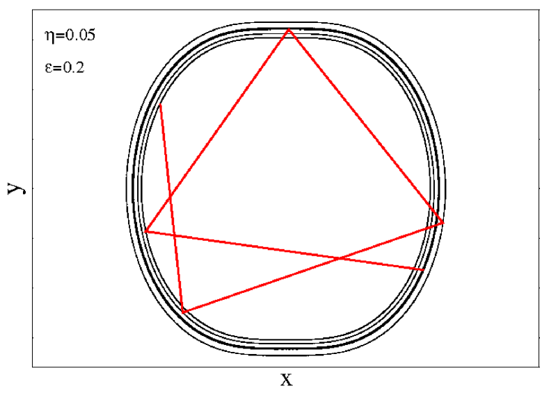
Figure 1: Plot of the boundary and a typical trajectory shown only for 6 snapshots of the boundary. The control parameters used were $\epsilon=0.2$, $\beta=\gamma=1.0$ and $\eta=0.05$.

shows a typical plot of the boundary and six collisions of a particle with the boundary.

To construct the mapping, we start with an initial condition $(\theta_{n},\alpha_{n},V_{n},t_{n})$. The Cartesian components of the boundary at the angular position $(\theta_{n},t_{n})$ are

$$X(\theta_{n},t_{n}) = [1+\eta\cos(t_{n})][1+\epsilon\cos(2\theta_{n})]\cos(\theta_{n})~{},$$ (1)

$$Y(\theta_{n},t_{n}) = [1+\eta\cos(t_{n})][1+\epsilon\cos(2\theta_{n})]\sin(\theta_{n})~{}.$$ (2)

The angle between the tangent of the boundary at the position $(X(\theta_{n}),Y(\theta_{n}))$ measured with respect to the horizontal line is

$$\phi_{n}=\arctan\left[Y^{\prime}(\theta_{n},t_{n})\over X^{\prime}(\theta_{n},t_{n})\right]~{},$$ (3)

where the expressions for both $X^{\prime}(\theta_{n},t_{n})$ and $Y^{\prime}(\theta_{n},t_{n})$ are written as

$$X^{\prime}(\theta_{n},t_{n}) = {dR(\theta_{n},t_{n})\over d\theta_{n}}\cos(\theta_{n})-R(\theta_{n},t_{n})\sin(\theta_{n}),$$ (4)

$$Y^{\prime}(\theta_{n},t_{n}) = {dR(\theta_{n},t_{n})\over d\theta_{n}}\sin(\theta_{n})+R(\theta_{n},t_{n})\cos(\theta_{n})~{},$$ (5)

with $dR(\theta_{n},t_{n})/d\theta_{n}=-2\epsilon[1+\eta\cos(t_{n})]\sin(2\theta_{n})$. Since the expressions for $\phi_{n}$ and $\alpha_{n}$ are known, the angle of the trajectory of the particle measured with respect to the positive X-axis is $(\phi_{n}+\alpha_{n})$. Such information allows us to write the particle’s velocity vector as

$$\overrightarrow{V}_{n}=|\overrightarrow{V_{n}}|[\cos(\phi_{n}+\alpha_{n})\widehat{i}+\sin(\phi_{n}+\alpha_{n})\widehat{j}]~{},$$ (6)

where $\widehat{i}$ and $\widehat{j}$ denote the unity vectors with respect to the X and Y axis, respectively. The position of the particle, as a function of time, for $t\geq t_{n}$, is given by

$$X_{p}(t) = X(\theta_{n},t_{n})+|\overrightarrow{V}_{n}|\cos(\phi_{n}+\alpha_{n})(t-t_{n})~{},$$ (7)

$$Y_{p}(t) = Y(\theta_{n},t_{n})+|\overrightarrow{V}_{n}|\sin(\phi_{n}+\alpha_{n})(t-t_{n})~{}.$$ (8)

We stress the sub-index $p$ denotes that such coordinates correspond to the particle. The distance of the particle measured with respect to the origin of the coordinate system is given by $R_{p}(t)=\sqrt{X^{2}_{p}(t)+Y^{2}_{p}(t)}$ and $\theta_{p}$ at ($X_{p}(t),Y_{p}(t)$) is $\theta_{p}=\arctan[Y_{p}(t)/X_{p}(t)]$. Therefore, the angular position at the next collision of the particle with the boundary, i.e. $\theta_{n+1}$, is numerically obtained by solving $R_{p}(\theta_{n+1},t_{n+1})=R_{b}(\theta_{n+1},t_{n+1})$. It means that the position of the boundary is the same as the position of the particle at the instant of the collision. The time $t_{n+1}$ is obtained by evaluating the expression

$$t_{n+1}=t_{n}+{{\sqrt{\Delta X^{2}+\Delta Y^{2}}}\over|\overrightarrow{V}_{n}|}~{},$$ (9)

where $\Delta X=X_{p}(\theta_{n+1},t_{n+1})-X(\theta_{n},t_{n})$ and $\Delta Y=Y_{p}(\theta_{n+1},t_{n+1})-Y(\theta_{n},t_{n})$. To obtain the new velocity we should note that the referential frame of the boundary is moving. Since we are considering inelastic collisions, the particle experiences a fractional loss of energy upon collision in both its normal and tangential components. Therefore, at the instant of collision, the following conditions must be matched

$$\overrightarrow{V^{\prime}}_{n+1}\cdot\overrightarrow{T}_{n+1} = \beta\overrightarrow{V^{\prime}}_{n}\cdot\overrightarrow{T}_{n+1}~{},$$ (10)

$$\overrightarrow{V^{\prime}}_{n+1}\cdot\overrightarrow{N}_{n+1} = -\gamma\overrightarrow{V^{\prime}}_{n}\cdot\overrightarrow{N}_{n+1}~{},$$ (11)

where the unitary tangent and normal vectors are

$$\overrightarrow{T}_{n+1} = \cos(\phi_{n+1})\widehat{i}+\sin(\phi_{n+1})\widehat{j}~{},$$ (12)

$$\overrightarrow{N}_{n+1} = -\sin(\phi_{n+1})\widehat{i}+\cos(\phi_{n+1})\widehat{j}~{}.$$ (13)

$\beta$ and $\gamma$ are damping coefficients, it means that the particle can loses velocity/energy upon collision in its normal component $(\gamma)$, tangential component $(\beta)$ or both. We consider both $\gamma\in[0,1]$ and $\beta\in[0,1]$. The completely inelastic collision happens when $\gamma=\beta=0$ and is not considered in this paper. On the other hand, when $\gamma=\beta=1$, corresponding to an elastic collision, all the results for the non-dissipative case are recovered. The upper prime indicates that the velocity of the particle is measured with respect to the moving boundary referential frame. At the new angular position $\theta_{n+1}$, we find that

$$\overrightarrow{V}_{n+1}\cdot\overrightarrow{T}_{n+1} = \beta\overrightarrow{V}_{n}\cdot\overrightarrow{T}_{n+1}+$$ (14)

$$+ (1-\beta)\overrightarrow{V}_{b}(t_{n+1})\cdot\overrightarrow{T}_{n+1}~{},$$

$$\overrightarrow{V}_{n+1}\cdot\overrightarrow{N}_{n+1} = -\gamma\overrightarrow{V}_{n}\cdot\overrightarrow{N}_{n+1}+$$ (15)

$$+ (1+\gamma)\overrightarrow{V}_{b}(t_{n+1})\cdot\overrightarrow{N}_{n+1}~{},$$

where $\overrightarrow{V}_{b}(t_{n+1})$ is the velocity of the boundary which is written as

$$\overrightarrow{V}_{b}(t_{n+1})={dR_{b}(t_{n+1})\over dt_{n+1}}[\cos(\theta_{n+1})\widehat{i}+\sin(\theta_{n+1})\widehat{j}]~{},$$ (16)

with

$${dR_{b}(t_{n+1})\over dt_{n+1}}=-\eta[1+\epsilon\cos(2\theta_{n+1})]\sin(t_{n+1})~{}.$$ (17)

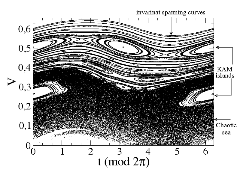
Figure 2: Phase space in the variables velocity and time for a time dependent oval billiard. The control parameters used were $\epsilon=0.2$, $\beta=\gamma=1.0$ and $\eta=0.05$. We assume as fixed the initial conditions $\alpha_{0}=\pi/2$ and $\theta_{0}=3\pi/2$.

Then we have

$$|\overrightarrow{V}_{n+1}|=\sqrt{(\overrightarrow{V}_{n+1}\cdot\overrightarrow{T}_{n+1})^{2}+(\overrightarrow{V}_{n+1}\cdot\overrightarrow{N}_{n+1})^{2}}~{}.$$ (18)

Finally, the angle $\alpha_{n+1}$ is written as

$$\alpha_{n+1}=\arctan\left[{\overrightarrow{V}_{n+1}\cdot\overrightarrow{N}_{n+1}\over\overrightarrow{V}_{n+1}\cdot\overrightarrow{T}_{n+1}}\right]~{}.$$ (19)

With this four dimensional mapping, we can explore now numerical results for the dynamics of the particle.

2.1 Numerical Results

In this section we discuss our numerical results. Just to remind, our main goal is to characterize a boundary crisis in a time-dependent oval-shaped billiard. To start, we show in Fig. 2 a typical phase space for a special set of initial conditions: $\alpha_{0}=\pi/2$ and $\theta_{0}=3\pi/2$. For such combination of initial condition and taken into account $\epsilon=0.2$ and $\eta=0.05$ the boundary has neutral curvature. With this particular choice of initial conditions, the phase space of the system is mixed. On the other hand, if we chose random $\alpha_{0}$ and $\theta_{0}$, the particle experiences the phenomenon of unlimited energy growth [36].

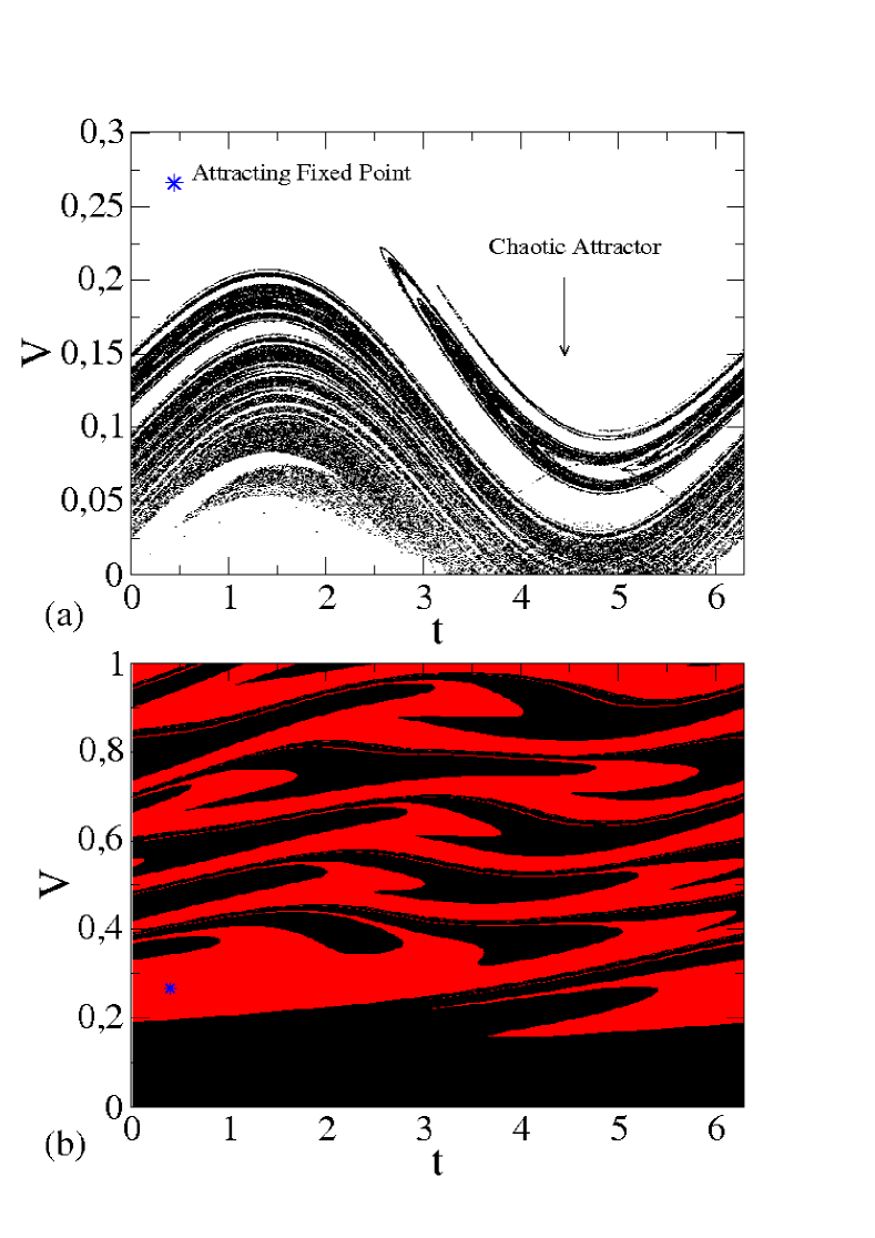
Figure 3: (Color online) (a) Attracting Fixed point indicated by a blue star ($\ast$) and chaotic attractor (set of black points); (b) Their corresponding basin of attraction. Black corresponds to the basin of attraction for the chaotic attractor and dark gray (red) of the attracting fixed point. The control parameters used were $\epsilon=0.2$, $\beta=0.25$, $\gamma=0.8899$ and $\eta=0.05$.

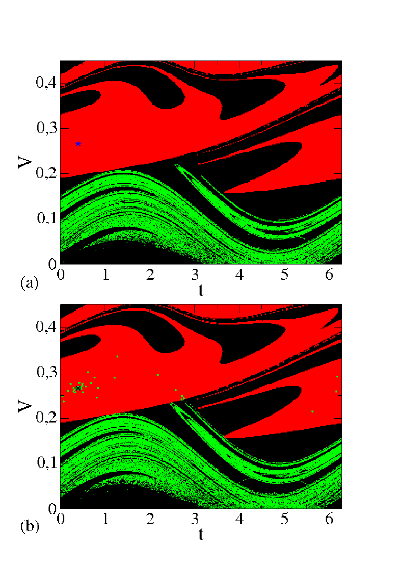
Figure 4: (Color online) Basin of attraction for the chaotic attractor and attracting fixed point (sink). The region in black corresponds to the basin of attraction of the chaotic attractor; the region in dark gray (red), denotes the basin of attraction of the attracting fixed point; light gray (green) in (a) identifies the chaotic attractor. The control parameters used to construct the basin of attraction were $\epsilon=0.2$, $\beta=0.25$, $\eta=0.05$ and $\gamma=0.8899$. The dissipation used in (a) the chaotic attractor were $\gamma=0.8899$ (before crisis, light gray (green)); (b) the chaotic transient were $\gamma=0.8906$ (after crisis, light gray (green)).

We now consider the situation where both damping coefficients $\beta\neq 1$ and $\gamma\neq 1$. We then keep fixed up to the end of the paper $\beta=0.25$. It implies that there is a high dissipation along the tangent component of the particle’s velocity. Results for different $\beta$ will be published elsewhere [37]. The parameter $\gamma$ is considered from the order of $\gamma=0.89$. It is shown in Fig. 3(a) the behavior of the attractors present in the system for the following combination of control parameters $\epsilon=0.2$, $\beta=0.25$, $\gamma=0.8899$ and $\eta=0.05$. We can see a chaotic attractor and an attracting fixed point. Figure 3(b) shows their corresponding basin of attraction. The procedure used to construct the basin of attraction was divide both $V$ and $t$ into windows of $500$ parts each, thus leading to a total of $2.5\times 10^{5}$ different initial conditions. Each initial condition was iterated up to $n=5\times 10^{6}$ collisions with the boundary. We see that only two attractors emerged for such combination of control parameters: sink and chaotic attractor. We stress that other attractors could in principle exist. If they exist however, their basin of attraction are too small to be obtained. It is clear that, after a very long number of collisions of the particle with the boundary, the velocity of the particle does not grow unlimitedly. Consequently, no Fermi acceleration is observed and we conclude that introduction of inelastic collisions worked out perfectly as a mechanism to suppress Fermi acceleration, as proposed in Ref. [38] for a stochastic 1-D system.

Let us now go ahead with the characterization of the boundary crisis [31, 32, 33]. It is well known in the literature that a saddle fixed point, in the plane $V\times t$ has two kinds of manifolds: (a) stable and (b) unstable. The unstable manifolds are formed by a family of trajectories that turn away from the saddle fixed point. One of them can form the chaotic attractor (or visit the region of the chaotic attractor after the event of crisis), while the other one moves towards an attracting fixed point. These manifolds are obtained from the iteration of the map $T$ with appropriate initial conditions. Similarly, the construction of stable manifolds are a little bit more complicated since the inverse of the mapping, say $T^{-1}$, must be obtained. The procedure for obtaining the stable manifolds is the same as that one used for the unstable manifolds, however, instead of iterating the map $T$ we must iterate its inverse $T^{-1}$. Since the stable manifolds generate the border of the basin of attraction of the chaotic attractor and attracting sink, a boundary crisis happens when a chaotic attractor touch the stable manifold due to a modification of the control parameter. As a consequence, there is a sudden and drastic destruction of the chaotic attractor and its basin of attraction.

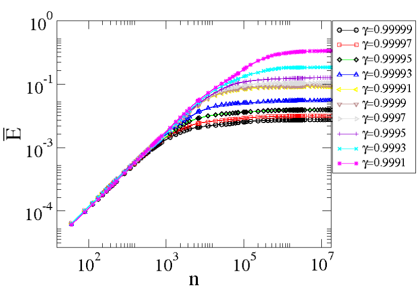
Figure 5: Behaviour of $\overline{E}\times n$ for different values of $\gamma$, as labeled in the figure. The control parameters used in the construction of the figure were $p=2$, $\epsilon=0.4$, $\beta=1$ and $\eta=0.001$.

It is shown in Fig. 4(a), two basins of attraction; one in black, corresponding to the basin of attraction of the chaotic attractor, and the other one in dark gray (red), denoting the basin of attraction of the attracting fixed point, and the chaotic attractor marked by light gray (green). If we increase the value of the parameter $\gamma$, which is equivalent to reduce the intensity of the dissipation, the two branches of the stable manifold touch, even crosses, the edges of the chaotic attractor, see Fig. 4 (b). Such behaviour is equivalent to a collision of the chaotic attractor with its own basin of attraction. Of course after the collision, there is a sudden destruction of chaotic attractor and its basin of attraction. We have observed such crisis for the control parameters $\epsilon=0.2$, $\beta=0.25$, $\eta=0.05$ and $\gamma=0.8906$. Other boundary crisis are observed for different combinations of control parameters, too. After the boundary crisis, the entire plane $V\times t$ (t mod ($2\pi$)) is the basin of attraction for a sink. Therefore, all initial conditions in such a region will converge to the sink. Additionally, for the regime of weak dissipation, the average energy, $\overline{E}_{i}={{1}\over{n+1}}\sum_{j=0}^{n}E_{i,j}$, grows for short iteration number and suddenly it bends towards a regime of saturation for long enough values of $n$ as can be seen in Fig. 5. Consequently, the mechanism of Fermi acceleration is suppressed in high as well as weak dissipation.

3 Conclusion

As a short remark, we have studied a classical version of a dissipative time-dependent oval-shaped billiard. The dissipation was introduced via damping coefficients for both the normal and tangential components of the particle’s velocity. For the regime of high tangential dissipation, we characterized an event of boundary crisis. For the regime of weak dissipation, we have shown that the average energy remains constant for long enough time. Such result allows us to confirm that the introduction of inelastic collisions is sufficient to suppress Fermi acceleration since all the initial conditions will converge to attractors located at low velocity domain.

References

- [1] G. Katz, M. A. Ratner, R. Kosloff, Phys. Rev. Lett. 98 (2007) 203006.
- [2] D. J. Tannor, A. Bartana, J. Phys. Chem. A 103 (1999) 10359 .
- [3] S. E. Sklarz, D. J. Tannor, N. Khaneja, Phys. Rev. A 69 (2004) 053408.
- [4] V. L’vov, A. Pomyalov, I. Procaccia, V. Tiberkevich, Phys. Rev. Lett. 92 (2004) 244503 .
- [5] P. Parmananda, M. Hildebrand, M. Eiswirth, Phys. Rev. E 56 (1997) 239.
- [6] J. K. Bhattacharjee, D. Thirumalai, Phys. Rev. Lett. 67 (1991) 196.
- [7] P. A. Cassak, M. A. Shay, Phys. Plasmas 16 (2009) 055704.
- [8] I. R. Senitzky, Phys. Rev. Lett. 15 (1965) 233.
- [9] M. N. Shneider, P. F. Barker, Phys. Rev. A 71 (2005) 053403.
- [10] R. Gommers, S. Bergamini, F. Renzoni, Phys. Rev. Lett. 95 (2005) 073003.
- [11] M. Steiner, M. Freitag, V. Perebeinos, J. C. Tsang, J. P. Small, M. Kinoshita, D. Yuan, J. Liu, P. Avouris, Nature Nanotechnology 4 (2009) 320.
- [12] Y. Zhao, C. Ma, G. Chen, Q. Jiang, Physical Review Letters 91 (2003) 175504.
- [13] W. V. Liu, W. C. Schieve, Phys. Rev. Lett. 78 (1997) 3278.
- [14] H.-P. Breuer, F. Petruccione, Phys. Rev. A 55 (1997) 3101.
- [15] K. Tsumura, T. Kunihiro, Physics Letters B 668 (2008) 425.
- [16] George M. Zaslavsky, Physics os Chaos in Hamiltonian Systems, Imperial college Press, London 1998.
- [17] E. D. Leonel, P. V. E. McClintock. Journal of Physics. A, Mathematical and General 39 (2006) 11399.
- [18] M. V. Berry, Eur. J. Phys. 2 (1981) 91.
- [19] M. Robnik, J. Phys. A: Math. Gen. 16 (1983) 3971.
- [20] M. Robnik, M. V. Berry, J. Phys. A: Math. Gen. 18 (1985) 1361.
- [21] S. O. Kamphorst, S. P. Carvalho, Nonlinearity 12 (1999) 1363.
- [22] R. Markarian, S. O. Kamphorst, S. P. de Carvalho, Commun. Math. Phys. 174 (1996) 661.
- [23] V. Lopac, I. Mrkonjić, D. Radić, Phys. Rev. E 66 (2002) 036202.
- [24] V. Lopac, I. Mrkonjić, N. Pavin, D. Radić, Physica D 217 (2006) 88.
- [25] D. F. M. Oliveira, E. D. Leonel, Commun Nonlinear Sci Numer Simulat (2010), doi:10.1016/j.cnsns.2009.05.044
- [26] A.K. Karlis, P.K. Papachristou, F.K. Diakonos, V. Constantoudis, P. Schmecher, Phys. Rev. Lett. 97 (2006) 194102.
- [27] E. Fermi, Phys. Rev. 75 (1949) 1169.
- [28] J. J. Barroso, M. V. Carneiro, E. E. N. Macau, Phys. Rev. E 79 (2009) 026206.
- [29] E. D. Leonel, D. F. M. Oliveira, R. E. de Carvalho, Physica A 386 (2007) 73.
- [30] L. D. Pustylnikov, Soviet. Math. Dokl. 35 (1987) 88.
- [31] E. D. Leonel, P. V. E. McClintock, J. Phys. A 38 (2005) L425.
- [32] C. Grebogi, E. Ott, J. A. Yorke, Phys. Rev. Lett. 48 (1982) 1507.
- [33] C. Grebogi, E. Ott, J. A. Yorke, Physica D 7 (1983) 181.
- [34] R. Egydio de Carvalho, C. V. Abud, F. C. Souza, Phys. Rev. E 77 (2008) 036204.
- [35] A. L. P. Livorati, D. G. Ladeira, E. D. Leonel, Phys. Rev. E 78 (2008) 056205.
- [36] E. D. Leonel, D. F. M. Oliveira, A. Loskutov, Chaos 19 (2009) 033142.
- [37] D. F. M. Oliveira, E. D. Leonel, Physica A 389 (2010) 1009.
- [38] E. D. Leonel, J. Phys. A: Math. Theor. 40 (2007) F1077.