Constraints from CMB in the Intermediate Brans-Dicke Inflation

Abstract

We study an intermediate inflationary stage in a Jordan-Brans-Dicke theory. In this scenario we analyze the quantum fluctuations corresponding to adiabatic and isocurvature modes. Our model is compared to that described by using the intermediate model in Einstein general relativity theory. We assess the status of this model in light of the seven-year WMAP data.

I Introduction

The inflationary paradigm inflation ; Linde has been confirmed as the most successful candidate for explaining the physics of the very early universe KKMR . This sort of scenarios has been successful in solving some of the puzzles of the standard cosmological model, such as the horizon, flatness and entropy problems, as well as providing for a mechanism to seed structure in the universe.

The source of inflation is a scalar field (the inflaton field), which plays an important role in providing a causal interpretation of the origin of the observed anisotropy of the cosmic microwave background radiation, and also distribution of large scale structure astro ; astro2 . The nature of this scalar field may be found by considering one of the extensions of the standard model of particle physics based on grand unified theories, supergravity, or some effective theory at low dimension of a more fundamental string theory.

The idea that inflation comes from an effective theory is in itself very appealing. The main motivation to study this sort of model comes from string/M-theory. This theory suggests that in order to have a ghost-free action high order curvature invariant corrections to the Einstein-Hilbert action must be proportional to the Gauss-Bonnet (GB) term BD . GB terms arise naturally as the leading order of the $\alpha$ expansion to the low-energy string effective action, where $\alpha$ is the inverse string tension KM . This kind of theory has been applied to the possible resolution of the initial singularity problem ART , also to the study of black-hole solutions Varios1 , and accelerated cosmological solutions Varios2 . In particular, it has been found Sanyal that for a dark energy model the GB interaction in four dimensions with a dynamical dilatonic scalar field coupling leads to a solution of the form $a(t)=a_{0}\exp({At^{f}})$, where the universe starts evolving with a decelerated exponential expansion. Here, the constant $A$ is given by $A=\frac{2}{\kappa n}$ and $f=\frac{1}{2}$, with $\kappa^{2}=8\pi G$, where $G$ is the newtonian gravitational constant, and $n$ an arbitrary constant.

We have the particular scenario called intermediate inflation Barrow1 , characterized for the scale factor evolving as $a(t)=a_{0}\exp(At^{f})$. In this model, the expansion of the universe is slower than standard de Sitter inflation ($a(t)=\exp(Ht)$), but faster than power law inflation ($a(t)=t^{p},\ p>1$). The intermediate inflationary model was introduced as an exact solution corresponding to a particular scalar field potential of the type $V(\phi)\propto\phi^{-4(f^{-1}-1)}$ (in the slow-roll approximation), where $0<f<1$. With this sort of potential it is possible in the slow-roll approximation to have a spectrum of density perturbations which presents a scale-invariant spectral index $n_{s}=1$, i.e. the so-called Harrison-Zel’dovich spectrum of density perturbations, provided $f$ takes the value of 2/3 Barrow2 . Even though this kind of spectrum is disfavored by the current Wilkinson Microwave Anisotropy Probe (WMAP) data B ; K ; H ; D , the inclusion of tensor perturbations, which could be present at some point by inflation and parametrized by the tensor-to-scalar ratio $r$, allows the conclusion that $n_{s}\geq 1$ providing that the value of $r$ is significantly nonzero ratio r . In fact, in Ref.Barrow3 was shown that the combination $n_{s}=1$ and $r>0$ is given by a version of the intermediate inflationary scenario in which the scale factor varies as $a(t)\propto e^{t^{2/3}}$ within the slow-roll approximation.

On the other hand, motivations also coming from string theory, there has been carried out a less standard theory of gravity, namely the so called scalar-tensor theory of gravity JBD ; BEPA ; varios3 ; varios4 . The archetypical theory associated with scalar-tensor models is the Jordan-Brans-Dicke (JBD) gravity JBD . The JBD theory is a class of model in which the effective gravitational coupling evolves with time. The strength of this coupling is determined by a scalar field, the so-called JBD field, which tends to the value $G^{-1}$. The origin of JBD theory is in Mach’s principle according to which the property of inertia of material bodies arises from their interactions with the matter distributed in the universe. In modern context, JBD theory appears naturally in supergravity models, Kaluza-Klein theories and in all known effective string actions F ; AChF ; FT1 ; FT2 ; CMPF ; CKP ; GSW .

In this paper we would like to study intermediate inflationary universe model in a JBD theory. We will write the Friedmann field equations, together with the corresponding scalar field equations (inflaton and JBD fields). The intermediate inflationary period of inflation will be consistently described in the slow-roll approximation. Scalar and tensor perturbations will be expressed in terms of the parameters that appear in our model, these parameters will be constrained by taking into account the WMAP five and seven year data.

The outline of the paper is as follows. The next section presents the field equations in the Einstein frame. In Section III we study the slow-roll approximation. Section IV deals with the calculations of cosmological scalar perturbations. Then we describe the quantum generation of fluctuations together with the spectrum of comoving curvature perturbations in section V. Section VI deals with tensor perturbations. Finally, in Section VII we conclude our findings.

II Background Equations in the Einstein Frame

A wide class of non-Einstein gravity models can be recast in the action Starobinsky2 :

$$S=\int\sqrt{-g}d^{4}x\left[\frac{1}{2\kappa^{2}}R+\frac{1}{2}g^{\mu\nu}\partial_{\mu}\chi\partial_{\nu}\chi-U(\chi)+\frac{1}{2}e^{-\gamma\kappa\chi}g^{\mu\nu}\partial_{\mu}\phi\partial_{\nu}\phi-e^{-\beta\kappa\chi}V(\phi)\right],$$ (1)

where $R$ is the Ricci scalar, $\kappa^{2}=8\pi G$, with $c=\hbar=1$, $\beta$ and $\gamma$ are constants, $\chi$ and $\phi$ are the dilaton and inflaton fields, respectively.

The Jordan-Brans-Dicke action in the Jordan frame is given as:

$$S=\int\sqrt{-\hat{g}}d^{4}x\left[\frac{\Phi_{BD}}{16\pi}{\cal\hat{R}}+\frac{\omega^{2}}{16\pi\Phi_{BD}}\hat{g}^{\mu\nu}\partial_{\mu}\Phi_{BD}\partial_{\nu}\Phi_{BD}+\frac{1}{2}\hat{g}^{\mu\nu}\partial_{\mu}\phi\partial_{\nu}\phi-V(\phi)\right],$$ (2)

and it is recovered by a conformal transformation Conformal on the action (1) with the condition $U(\chi)=0$

$$g_{\mu\nu}=\Omega^{2}\hat{g}_{\mu\nu}\ \ \ \ \ \textrm{and}\ \ \ \ \ \Omega^{2}\equiv\frac{\kappa^{2}}{8\pi}\Phi_{BD}\equiv e^{\gamma\kappa\chi},$$ (3)

for $\beta=2\gamma=\frac{2}{\sqrt{\omega+\frac{3}{2}}}$. $\Phi_{BD}$ is the Brans-Dicke field and $\omega$ is the Brans-Dicke parameter.

Observational measurements ObsWill ; ObsBertotti constraint the BD parameter to be very large $\omega\gg 1$. On the other hand, the BD field remains very close to a constant after inflation, in the radiation and matter domination eras JBD . In order to recover the right value of the newtonian gravitational constant after inflation we will consider $\chi$ equals to zero at the end of the inflationary stage.

From the action (1) in a flat Friedmann-Robertson-Walker (FRW) metric, tacking $U(\chi)=0$, we get the following set of field equations:

$$\ddot{\chi}+3H\dot{\chi}+\frac{\gamma\kappa}{2}e^{-\gamma\kappa\chi}\dot{\phi}^{2}-\beta\kappa e^{-\beta\kappa\chi}V(\phi) = 0,$$ (4)

$$\ddot{\phi}+3H\dot{\phi}-\gamma\kappa\dot{\chi}\dot{\phi}+e^{(\gamma-\beta)\kappa\chi}V^{\prime}(\phi) = 0,$$ (5)

$$3H^{2}-\kappa^{2}\left(\frac{1}{2}\dot{\chi}^{2}+\frac{1}{2}e^{-\gamma\kappa\chi}\dot{\phi}^{2}+e^{-\beta\kappa\chi}V(\phi)\right) = 0,$$ (6)

where overdots denote derivatives with respect to $t$ and a prime denotes derivative respect to the scalar field $\phi$, $H\equiv\frac{\dot{a}(t)}{a(t)}$ is the cosmic expansion rate and $a(t)$ is the scale factor. In the next section we will solve the set of equations Eqs.(4)-(6) in the slow-roll approximation.

III The slow-roll approximation

The slow-roll regime of an inflationary era is presented when $\left|\frac{\dot{H}}{H^{2}}\right|\ll 1$ and $\left|\frac{\ddot{H}}{\dot{H}H}\right|\ll 1$ Liddle-Lyth-0 . These conditions into Eqs.(4)-(6) impose the constraints:

$$\frac{1}{2}e^{-\gamma\kappa\chi}\dot{\phi}^{2}+\frac{1}{2}\dot{\chi}^{2} \ll e^{-\beta\kappa\chi}V(\phi),$$ (7)

$$\ddot{\phi}-\gamma\kappa\dot{\chi}\dot{\phi} \ll H\dot{\phi},$$ (8)

$$\ddot{\chi}+\frac{1}{2}\gamma\kappa e^{-\gamma\kappa\chi}\dot{\phi}^{2} \ll H\dot{\chi},$$ (9)

which transform the set of field equations, Eqs.(4)-(6), into the equations:

$$3H\dot{\chi}-\beta\kappa e^{-\beta\kappa\chi}V(\phi) = 0,$$ (10)

$$3H\dot{\phi}+e^{(\gamma-\beta)\kappa\chi}V^{\prime}(\phi) = 0,$$ (11)

$$3H^{2}-\kappa^{2}e^{-\beta\kappa\chi}V(\phi) = 0.$$ (12)

From this set of differential equations we easily realize that $\chi$ is given by:

$$\chi=\frac{\beta}{\kappa}\ln\left(\frac{a}{a_{b}}\right)+\chi_{b},$$ (13)

where the subscript $b$ will denote values at the beginning of the inflationary epoch.

By choosing an ansatz for the potential as $V(\phi)=V_{0}\phi^{n}$, from Eqs.(10)-(12) we obtain:

$$\phi^{2}-\phi_{b}^{2}=\frac{2ne^{\gamma\kappa\chi_{b}}}{\beta\gamma\kappa^{2}}\left(1-\left(\frac{a}{a_{b}}\right)^{\beta\gamma}\right)\ \ \ \ \ \textrm{and}\ \ \ \ \ e^{\gamma\kappa\chi}=e^{\gamma\kappa\chi_{b}}+\frac{\beta^{2}\kappa^{2}f}{16(1-f)}\left(\phi^{2}-\phi_{b}^{2}\right).$$ (14)

For the specific case of a Jordan-Brans-Dicke theory, where $\gamma=\frac{\beta}{2}$, we find:

$$a(t)=a_{b}\left(\frac{1+\frac{A}{p}t^{f}}{1+\frac{A}{p}t_{b}^{f}}\right)^{p}\ \ \ \ \ \textrm{and}\ \ \ \ \ \phi(t)=\left(\frac{8\sqrt{V_{0}}(1-f)t}{\sqrt{3}\kappa f^{2}}\right)^{\frac{f}{2}}$$ (15)

with $p\equiv\frac{2}{\beta^{2}}$, $f\equiv\frac{4}{4-n}$, $A\equiv-\frac{2}{(1+C_{2})\beta^{2}}\left(-\frac{C_{1}C_{2}}{f}\right)^{f}$, $t_{b}\equiv-\frac{f}{C_{1}C_{2}}$, $C_{1}\equiv e^{-\gamma\kappa\chi_{b}}\frac{\sqrt{V_{0}}\beta^{2}\kappa\phi_{b}^{n/2}}{2\sqrt{3}}$ and $C_{2}\equiv-e^{\gamma\kappa\chi_{b}}\frac{16(1-f)}{f\beta^{2}\kappa^{2}\phi_{b}^{2}}$.

The parameter $A$ in Eq.(15) has to be positive in order to get an increasing scale factor function. Consequently, we have the following constraints: $C_{2}<-1$, $0<f<1$ and $n<0$. In this case the potential $V(\phi)$ does not have a minimum and therefore a nonstandard way of reheating in the universe is required Curvaton .

From here on it is assumed $\gamma=\frac{\beta}{2}$ although sometimes $\gamma$ is preserved to shorten the length of the equations.

We note that the scale factor in Eq.(15) is a generalization of the scale factor corresponding to intermediate inflation in the Einstein theory Barrow1 , in the case $p\rightarrow\infty$ we recover $a(t)\propto e^{At^{f}}$. On the other hand, the authors of Ref.LaSteinhardt found the same form for $a(t)$ when they first studied a cosmological model in a JBD theory, extended inflation.

The number of e-folds between any time $t$ and the beginning of inflation $t_{b}$ is:

$$N\equiv\ln\left(\frac{a}{a_{b}}\right)=p\ln\left(\frac{1+\frac{A}{p}t^{f}}{1+\frac{A}{p}t_{b}^{f}}\right).$$ (16)

$N$ is always lower than the number of e-folds that we would get in an intermediate inflationary model in the Einstein theory Barrow-Liddle . Expression (16) converges to the Einstein case in the limit $p\rightarrow\infty$.

It is well known that an intermediate stage of inflation needs an additional mechanism to bring inflation to an end Barrow3 . We will consider that this mechanism starts after $N_{T}$ e-folds since the beginning of inflation. We normalize $\chi$ in such a way that after $N_{T}$ e-folds the value of the field $\chi$ becomes zero, therefore $\chi_{b}=-\frac{\beta}{\kappa}N_{T}$. We assume that the value of $\chi$ remains zero after that time in order to fulfill the condition $\Phi_{BD}=\frac{1}{G}$ after inflation.

It is convenient to calculate the so-called slow-roll parameters:

$$\epsilon \equiv -\frac{\dot{H}}{H^{2}}=\frac{\beta^{2}}{2}+e^{\gamma\kappa\chi}\frac{1}{2\kappa^{2}}\left(\frac{V^{\prime}}{V}\right)^{2},$$ (17)

$$\eta \equiv -\frac{\ddot{H}}{\dot{H}H}=-2\epsilon+\frac{7\beta^{2}}{2}-\frac{3\beta^{4}}{4\epsilon}+e^{\gamma\kappa\chi}\left(\frac{2}{\kappa^{2}}-\frac{\beta^{2}}{\epsilon\kappa^{2}}\right)\frac{V^{\prime\prime}}{V},$$ (18)

which will be useful in the study of the perturbations of the model. We recall that $\epsilon<1$ implies $\ddot{a}>0$, i.e. it guarantees the existence of an inflationary period.

From Eqs.(14) and (17) we note that $\epsilon$ is a decreasing function of time. Following Refs.Barrow3 ; delCampo we assume that the intermediate inflationary era begins at the earliest possible stage when $\epsilon=1$, which corresponds to:

$$t_{b}=\left(\frac{2(1-f)}{A(2f-\beta^{2})}\right)^{\frac{1}{f}},\ \ \ \ \phi_{b}=\frac{(1-f)}{f\kappa}\frac{4e^{\frac{\beta\kappa\chi_{b}}{4}}}{\sqrt{2-\beta^{2}}},\ \ \ \ V_{0}=\frac{3A^{\frac{2}{f}}f^{4}\kappa^{2}e^{\frac{\beta\kappa\chi_{b}}{f}}}{4^{3-\frac{3}{f}}(1-f)^{2}}\left(\frac{(1-f)\left(2f-\beta^{2}\right)}{f^{2}\left(2-\beta^{2}\right)\kappa^{2}}\right)^{\frac{2}{f}}.$$ (19)

We note that in the limit $\beta\rightarrow 0$ the expressions for $\phi(t)$ in Eq.(15), $\epsilon$ in Eq.(17) and $\eta$ in Eq.(18) go to the standard slow-roll relations corresponding to the intermediate inflationary universe model Barrow3 , as well as the expression for $V(\phi)$, where $V_{0}\rightarrow\frac{3A^{2}f^{2}}{\kappa^{2}}\left(\frac{8A(1-f)}{f\kappa^{2}}\right)^{2\left(\frac{1-f}{f}\right)}$.

We can check the consistency of the slow-roll approximation numerically. We get the solutions to the Eqs.(4)-(6) and compare with the solutions to Eqs.(10)-(12) (see FIG.1). The initial values for $\dot{\phi}(t)$ and $\dot{\chi}(t)$ in the exact solution were set from the slow-roll differential equations (10) and (11). We can see from FIG.1 that the slow-roll approximation for the given parameters is a very good approximation, this is also valid for the other parameters in the considered ranges.

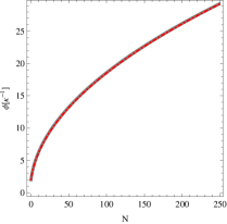
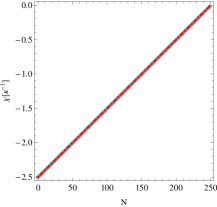
Figure 1: The panels show 250 e-folds of inflation for $f=0.7$ and $\beta=0.01$, the exact solutions to Eqs.(4)-(6) coincides with the solutions for these equations in the slow-roll approximation (dotdashed line). For the last 100 e-folds the error in use the slow-roll approximation is less than 1$\%$.

IV Linear Order Scalar Perturbations

We analyze the cosmological scalar perturbations in the longitudinal gauge Mukhanov , we consider the perturbed metric to be:

$$ds^{2}=(1+2\Phi)dt^{2}-a(t)^{2}(1-2\Psi)\delta_{ij}dx^{i}dx^{j}.$$ (20)

When we introduce this perturbed metric into the Einstein field equations with two scalar fields ($\phi$ and $\chi$) we get the following set of linear order perturbed field equations:

$$\Phi=\Psi$$ (23)

$$\dot{\Phi}+H\Phi=\frac{\kappa^{2}}{2}\left(\dot{\chi}\delta\chi+e^{-\gamma\kappa\chi}\dot{\phi}\delta\phi\right),$$

$$\ddot{\delta\chi}+3H\dot{\delta\chi}+\left(\frac{k^{2}}{a^{2}}-\frac{(\gamma\kappa)^{2}}{2}e^{-\gamma\kappa\chi}\dot{\phi}^{2}+(\beta\kappa)^{2}e^{-\beta\kappa\chi}V(\phi)\right)\delta\chi+\gamma\kappa e^{-\gamma\kappa\chi}\dot{\phi}\dot{\delta\phi}$$

$$-\beta\kappa e^{-\beta\kappa\chi}V^{\prime}(\phi)\delta\phi=2(\ddot{\chi}+3H\dot{\chi})\Phi+\dot{\Phi}\dot{\chi}+3\dot{\Psi}\dot{\chi}+\gamma\kappa e^{-\gamma\kappa\chi}\dot{\phi}^{2}\Phi,$$

and $$\ddot{\delta\phi}+(3H-\gamma\kappa\dot{\chi})\dot{\delta\phi}+\left(\frac{k^{2}}{a^{2}}+e^{(\gamma-\beta)\kappa\chi}V^{\prime\prime}(\phi)\right)\delta\phi-\gamma\kappa\dot{\phi}\dot{\delta\chi}$$ (24)

$$+(\gamma-\beta)\kappa V^{\prime}(\phi)e^{(\gamma-\beta)\kappa\chi}\delta\chi=2(\ddot{\phi}+3H\dot{\phi})\Phi+\dot{\Phi}\dot{\phi}+3\dot{\Psi}\dot{\chi}-2\gamma\kappa\dot{\phi}\dot{\chi}\Phi,$$

where $\delta\phi$ and $\delta\chi$ are gauge invariant fluctuations of the respective fields and $k$ stands for the Fourier space decomposition.

We use the slow-roll approximation in Eqs.(23)-(24) and given that we are interested in the non-decreasing adiabatic and isocurvature modes on large scales $k\ll aH$ Liddle-Lyth , we can consistently neglect the terms containing $\dot{\Phi}$ and those terms containing second order time derivatives. Under these approximations Eqs.(23)-(24) reduce to:

$$\Phi=\frac{\kappa^{2}}{2H}\left(\dot{\chi}\delta\chi+e^{-\gamma\kappa\chi}\dot{\phi}\delta\phi\right)=\frac{\beta\kappa}{2}\delta\chi-\frac{V^{\prime}(\phi)}{2V(\phi)}\delta\phi,$$ (26)

$$3H\dot{\delta\chi}+(\beta\kappa)^{2}e^{-\beta\kappa\chi}V(\phi)\delta\chi-\beta\kappa e^{-\beta\kappa\chi}V^{\prime}(\phi)\delta\phi=2\beta\kappa e^{-\beta\kappa\chi}V(\phi)\Phi,$$

and $$3H\dot{\delta\phi}+e^{(\gamma-\beta)\kappa\chi}V^{\prime\prime}(\phi)\delta\phi+(\gamma-\beta)\kappa V^{\prime}(\phi)e^{(\gamma-\beta)\kappa\chi}\delta\chi=-2e^{(\gamma-\beta)\kappa\chi}V^{\prime}(\phi)\Phi.$$ (27)

The authors in Ref.Starobinsky ; Chiba-Sugiyama-Yokoyama have found a solution to the set of Eqs.(26)-(27):

$$\frac{\delta\chi}{\dot{\chi}}=\frac{C_{1}}{H}-\frac{C_{3}}{H},$$ (29)

$$\frac{\delta\phi}{\dot{\phi}}=\frac{C_{1}}{H}+\frac{C_{3}}{H}(e^{-\gamma\kappa\chi}-1),$$

and $$\Phi=-C_{1}\frac{\dot{H}}{H^{2}}+C_{3}\left(\frac{(1-e^{\gamma\kappa\chi})}{2\kappa^{2}}\left(\frac{V^{\prime}(\phi)}{V(\phi)}\right)^{2}-\frac{\beta^{2}}{2}\right),$$ (30)

where $C_{1}$ and $C_{3}$ are two integration constants related with the initial values of $\delta\phi$, $\delta\chi$, $\phi$ and $\chi$. The terms proportional to $C_{1}$ and $C_{3}$ represent adiabatic and isocurvature modes, respectivelyStarobinsky2 . The isocurvature nature of the term proportional to $C_{3}$ is guaranteed by the fact that the second term in Eq.(30) is vanishingly small after inflation when $\chi(t)\approx 0$.

In order to get the spectrum of scalar perturbations we introduce the gauge-invariant quantity named the comoving curvature perturbation, ${\cal R}$ Garcia-Bellido-Wands :

$${\cal R}=\Psi-\frac{H}{\dot{H}}\left(\dot{\Psi}+H\Phi\right)=-\frac{H^{2}}{\dot{H}}\Phi,$$ (31)

where the latter expression is valid for large scales in the slow-roll regime. By substituting $\Phi$ given by Eq.(30) into Eq.(31) we obtain:

$${\cal R}=C_{1}-C_{3}W,$$ (32)

with $W=1-\left(e^{\gamma\kappa\chi(t)}+\beta^{2}\kappa^{2}\left(\frac{V(\phi)}{V^{\prime}(\phi)}\right)^{2}\right)^{-1}$.

As we see from Eq.(32), the term $W$ is responsible for the change of ${\cal R}$ during the inflationary stage. For intermediate inflation in a JBD theory we can calculate $W$ by using Eqs.(13), (14) and (16) as well as the definition of $V(\phi)$:

$$W(N)=1+\frac{e^{\frac{N_{T}\beta^{2}}{2}}(1-f)(2-\beta^{2})}{2f-\beta^{2}-e^{\frac{N\beta^{2}}{2}}(2-\beta^{2})},$$ (33)

where $N_{T}$ is the total amount of e-folds of inflation for which the value of $\chi$ goes to zero. Here we have used the number of e-folds $N$ to describe time evolution because it is more convenient in the subsequent analysis.

We note that the case $\beta=0$ corresponds to $W=0$, which is expected because when the BD parameter is zero there is only one scalar field driving inflation, and in that case the comoving curvature perturbation $\cal{R}$ remains constant on large scales Mukhanov .

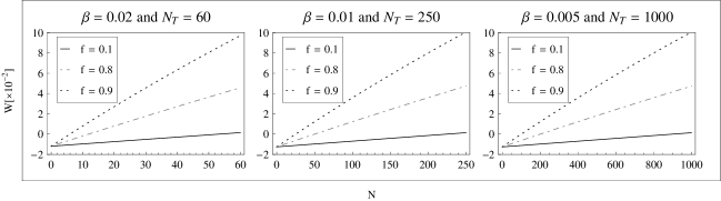
Figure 2: The variation of the function $W$ during the intermediate inflationary stage for different values of $\beta$ and $f$. In order to have $|{W}|<0.1$ the maximum number of e-folds allowed $N_{T}$ changes depending on $\beta$ for $0<f<1$.

The current observational constraints bring $\beta$ to an upper limit given by $\beta\leq 0.02$ ObsBertotti . We see from FIG. 2 that for a wide range of $N_{T}$ we can find values for $\beta$ and $f$ in the allowed ranges in such a way that $|W|<0.1$. For example, for $\beta=0.01$, $f=0.8$ and $N_{T}\leq 250$ we get $|W|<0.05$.

Given that the constants $C_{1}$ and $C_{3}$ are related to the initial values of the perturbed fields it is expected they to be of the same order Starobinsky2 , then to impose $|W|<0.1$ guarantees that the variation of ${\cal R}$ during inflation due to the presence of isocurvature perturbations is small, i.e. for a given $\beta$ and $f$ we can find a maximum $N_{T}$ value for which $|W|<$ desired value.

In the following we will consider for the comoving curvature perturbation ${\cal R}\approx C_{1}$, i.e. ${\cal R}$ remains constant after a given scale $k$ leaves the Hubble horizon during inflation. Furthermore, we will assume that the mechanism which is needed to properly finish inflation is not going to modify the results for ${\cal R}$.

In FIG.3 we plot the comoving curvature perturbation, the exact solution and the solution in the slow-roll approximation are compared. We confirmed, for the allowed range of parameters for $\beta$, $f$ and $N_{T}$, that the slow-roll approximation is adequated when we set the initial values of $\dot{\phi}$, $\dot{\chi}$, $\dot{\delta{\phi}}$ and $\dot{\delta\chi}$ from the equations in the slow-roll approximation.

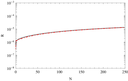
Figure 3: The figure shows a comparison of the comoving curvature perturbation between the solutions to the exact perturbed field equations and the solutions to these equations in the slow-roll approximation. For the last 100 e-folds the error in use the slow-roll approximation is less than 5$\%$. The values for the parameters and the initial conditions are the same considered in FIG.1. We have normalized to get $P_{\cal R}=2.3\times 10^{-9}$ at the crossing time when $N_{*}=50$ e-folds.

V Quantum Generation of Fluctuations and Spectrum of Curvature Perturbation

The value of the constant $C_{1}$ in the slow-roll approximation and for large scales ($k\ll aH$) is gotten from Eqs.(29) and (29):

$$C_{1}=He^{\gamma\kappa\chi}\left(\frac{\delta\chi}{\dot{\chi}}\left(e^{-\gamma\kappa\chi}-1\right)+\frac{\delta\phi}{\dot{\phi}}\right).$$ (34)

The expectation values of the scalar field perturbations $\delta\phi$ and $\delta\chi$ are given by random gaussian variables when they cross outside the Hubble radius ($k\approx a_{*}H_{*}$) Mukhanov , these are given by:

$$\langle|\delta\phi_{*}|^{2}\rangle=\frac{H_{*}^{2}}{2k^{3}}e^{\gamma\kappa\chi_{*}}\ \ \ \ \ \textrm{and}\ \ \ \ \ \langle|\delta\chi_{*}|^{2}\rangle=\frac{H_{*}^{2}}{2k^{3}}$$ (35)

respectively, here the subscript $*$ denotes the crossing time and the brackets the expectation value of the respective random variable.

The spectrum of the comoving curvature perturbation ${\cal R}$ is defined by Garcia-Bellido-Wands :

$$P_{{\cal R}}(k)=\frac{4\pi k^{3}}{(2\pi)^{3}}\langle|{\cal R}|^{2}\rangle.$$ (36)

From the discussion in Section IV and Eqs.(34) and (35) we obtain:

$$P_{{\cal R}}(k_{*})=\frac{4\pi k_{*}^{3}}{(2\pi)^{3}}\langle|C_{1}|^{2}\rangle=\left[\frac{H^{2}e^{2\gamma\kappa\chi}}{(2\pi)^{2}}\left(\left(e^{-\gamma\kappa\chi}-1\right)^{2}\frac{H^{2}}{\dot{\chi}^{2}}+\frac{H^{2}e^{\gamma\kappa\chi}}{\dot{\phi}^{2}}\right)\right]_{t_{*}}.$$ (37)

We note that the presence of a second scalar field during inflation modifies the form of the standard spectrum Starobinsky2 , the standard form Linde is recovered when we take the limit $\gamma\rightarrow 0$. In terms of $\chi$ and the parameters of the model, the spectrum becomes:

$$P_{{\cal R}}(k_{*})=\frac{\kappa^{2}}{12}V_{0}\phi_{*}^{n}\left(\left(1-e^{-\frac{1}{2}\beta\kappa\chi_{*}}\right)^{2}\frac{\kappa^{2}}{\beta^{2}}+e^{-\frac{1}{2}\beta\kappa\chi_{*}}\frac{\phi_{*}^{2}}{n^{2}}\right),$$ (38)

where $n=4\left(\frac{f-1}{f}\right)$, $\phi_{*}$ is given by Eq.(14) in terms of $\chi_{*}$ and $\chi_{*}$ is related to $N_{*}$ by Eq.(13) where $\chi_{b}=-\frac{\beta}{\kappa}N_{T}$.

From the seven-year WMAP data we know that the amplitude of the spectrum is $P_{\cal R}(k_{*})=2.43\times 10^{-9}$ for a scale $k_{*}=0.002\textrm{Mpc}^{-1}$ WMAP . By imposing this constraint in Eq.(38) we can get the value of the constant $V_{0}$ for given values of the parameters $\beta$, $f$, $N_{T}$ and $N_{*}$. In FIG. 4 we show the value of the parameter $A$, related to $V_{0}$ through Eq.(19).

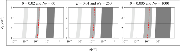
Figure 4: The panels show the value of $A$ in units $\kappa^{-f}$. The stripes in each panel represents from darkest to lightest $f=0.4,0.6,0.8$. The dashed line corresponds to a scale $k=0.002\textrm{Mpc}^{-1}$ leaving the horizon after 10 e-folds since the beginning of inflation for different sets of parameters.

The scale dependence of the spectrum is characterized by the spectral index $n_{s}(k)$ whereas the scale dependence of the spectral index is given by the running $\alpha_{s}$ Liddle-Lyth-0 .

We can calculate the spectral index and the running for scalar perturbations as:

$$n_{s}(k_{*}) \equiv 1+\frac{d\ln P_{{\cal R}}}{d\ln k}=1-4\epsilon+\eta+\frac{\beta^{2}}{2}Z_{1},$$ (39)

$$\alpha_{s}(k_{*}) \equiv \frac{dn_{s}}{d\ln k}=-8\epsilon^{2}+5\epsilon\eta-\xi^{2}+\frac{\beta^{4}}{4}Z_{2},$$ (40)

where we have used $d\ln k=dN$ and

$$Z \equiv e^{\frac{N\beta^{2}}{2}}\left(2-\beta^{2}\right),\ \ \ \ \ \ \ \ \ Z_{0}\equiv e^{\frac{N_{T}\beta^{2}}{2}}\left(2-\beta^{2}\right),\ \ \ \ \ \ \ \ \ \xi^{2}\equiv\epsilon\eta-\frac{\sqrt{2\epsilon}}{\kappa}\frac{d\eta}{d\phi}\sqrt{\frac{-2f+Z+\beta^{2}}{Z_{0}(1-f)}},$$

$$Z_{1} \equiv 1-\frac{fZ}{f(Z-2)+\beta^{2}}+\frac{Z}{Z-2f+\beta^{2}}+\frac{Z^{2}+(f-1)Z_{0}^{2}}{(Z-Z_{0})^{2}+f\left(2Z(Z_{0}-1)-Z_{0}^{2}\right)+Z\beta^{2}},$$

$$Z_{2} \equiv -1+\frac{f^{2}Z^{2}}{\left(f(Z-2)+\beta^{2}\right)^{2}}+\frac{fZ}{(1-f)\left(f(Z-2)+\beta^{2}\right)}-\frac{Z}{(1-f)\left(-2f+Z+\beta^{2}\right)}$$

$$- \frac{\left(Z^{2}+(f-1)Z_{0}^{2}\right)^{2}}{\left((Z-Z_{0})^{2}+f\left(2Z(Z_{0}-1)-Z_{0}^{2}\right)+Z\beta^{2}\right)^{2}}+\frac{Z^{2}-(f-1)Z_{0}^{2}}{(Z-Z_{0})^{2}+f\left(2Z(Z_{0}-1)-Z_{0}^{2}\right)+Z\beta^{2}}.$$

We note that both Eqs.(39) and (40) reduce to the result in the Einstein theory when $\beta\rightarrow 0$ Barrow3 .

VI Tensor Perturbations

In addition to the scalar curvature perturbation, tensor perturbations can also be generated from quantum fluctuations during inflation Mukhanov . The tensor perturbations do not couple to matter and consequently they are only determined by the dynamics of the background metric, so the standard results for the evolution of tensor perturbations of the metric remains valid. The two independent polarizations evolve like minimally coupled massless fields with spectrum Mukhanov :

$$P_{{\cal T}}(k_{*})=8\kappa^{2}\left(\frac{H}{2\pi}\right)^{2}_{t_{*}}.$$ (41)

From Eq.(37) and Eq.(41) we can determine the tensor to scalar ratio $r$:

$$r(k_{*})=\frac{P_{{\cal T}}}{P_{{\cal R}}}=8\kappa^{2}\left[e^{2\gamma\kappa\chi}\left(\left(e^{-\gamma\kappa\chi}-1\right)^{2}\frac{H^{2}}{\dot{\chi}^{2}}+\frac{H^{2}e^{\gamma\kappa\chi}}{\dot{\phi}^{2}}\right)\right]_{t_{*}}^{-1},$$ (42)

which in terms of $Z$ is rewritten as:

$$r(k_{*})=\frac{8(1-f)Z_{0}^{2}\beta^{2}}{(Z_{*}-Z_{0})^{2}+f\left(2Z_{*}(-1+Z_{0})-Z_{0}^{2}\right)+Z_{*}\beta^{2}},$$ (43)

and it is reduced to $16\epsilon$ in the limit $\beta\rightarrow 0$ consistent with Ref.Barrow3 .

Our analysis has been done in the Einstein frame but the physical results have to be interpreted in the Jordan physical frame. The authors of Ref.Starobinsky2 analyze this issue and they conclude that both frames are equivalent given that the JBD field varies extremely slowly in the post-inflationary universe, then the adiabatic fluctuations and the tensor perturbations are described by the same formula in both frames.

As we can see from Eqs.(39) and (43) $n_{s}$ and $r$ only depends on the parameters $f$, $N_{T}$, $\beta$ and $N_{*}$. FIG. 5 shows the behavior for the curve $r(n_{s})$ for several choices of the parameters. When we take different values for the total amount of inflation for a given $\beta$ and $f$, the curves in the plane $n_{s}-r$ have different curvature but they have the same origin in the bottom of the plot. When we take the same amount of total inflation but different values for $\beta$ for a given $f$, the curves do not have the same origin.

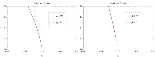
Figure 5: Trajectories for different values of the parameter $\beta$ and $N_{T}$ in the $n_{s}-r$ plane. Here $N_{*}$ is a parameter which defines the curve

FIG. 6 shows the dependence of the tensor to scalar ratio on the spectral index for different values of the parameters $\beta$, $f$ and the corresponding maximum $N_{T}$. We should note from Eqs.(39) and (43) that these curves are parametrized by the parameter $N_{*}$. For $\beta\leq 0.001$ there is not significant difference with the predictions in the case of intermediate inflation in the Einstein theory Barrow3 . The only difference seems to be the improvement in the observational constraints to the allowed plane $n_{s}-r$ since WMAP3 to WMAP7.

For $\beta=0.01$, $0.4\leq f<0.8$ is well supported by the data. But there exist a theoretical limit for the model in the maximum number of e-folds of inflation allowed (represented by the yellow line in the left panel of FIG. 6), $N_{T}\leq 250$.

In the case $\beta=0.02$, the maximum value for $\beta$ constrained from tests of general relativity ObsWill ; ObsBertotti , we can have at most 60 e-folds of inflation in order to have a comoving curvature perturbation close to a constant. This constraint in the number of e-folds exclude $f=0.4$ to be supported by the data but it still allow $0.5\leq f<0.8$ to be well supported.

We see from FIG. 6 that the curve $r=r(n_{s})$ enters the $95\%$ confidence region for $r\leq 0.41$ which in terms of the number of e-folds (at the time when a given scale leaves the horizon) means $N>78$ for $f=0.4$, $N>48$ for $f=0.5$, $N>29$ for $f=0.6$ and $N>16$ for $f=0.7$. There are not significant differences for the values of $\beta$ considered in FIG. 6. On the other hand, we have to consider at least 50 e-folds of inflation to push the perturbations to observable scales Liddle-Lyth-2 , which seems to exclude models for $\beta=0.02$ and $f<0.7$.

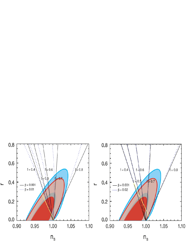
Figure 6: Trajectories for different values of the parameter $\beta$ and $f$ in the $n_{s}-r$ plane. We compare with the WMAP data (five and seven years). The two contours correspond to the $68\%$ and $95\%$ levels of confidence WMAP2 . The left panel shows $N_{T}=250$ e-folds for $\beta=0.01$ whereas the right panel is for $N_{T}=60$ e-folds for $\beta=0.02$.

VII Conclusion

We have studied in detail the intermediate inflationary scenario in the context of a JBD theory. This study was realized in the Einstein frame, but the physical results have to be interpreted in the Jordan physical frame. In this respect, it has been considered that both frames are equivalent, providing that the JBD field varies extremely slowly in the post-inflationary stage of the universe Starobinsky2 . In this way, the adiabatic fluctuations and the tensor perturbations are described equally in both frames. This allows to obtain explicit expressions for the corresponding power spectrum of the curvature perturbations $P_{{\cal R}}$, tensor perturbation $P_{{\cal T}}$, tensor-scalar ratio $r$, scalar spectral index $n_{s}$, and its running $\alpha_{s}$.

In this work the aim has been to study which set of parameters $\beta$, $f$ and $N_{T}$ allow us to get a dominant contribution of the adiabatic mode to the power spectrum of scalar perturbations. In order to do that we have restricted the maximum number of e-folds allowed by the model, $N_{T}$, for a given set of parameters $\beta$ and $f$. For a given value of $\beta$ and $0<f<1$ we get ${\cal R}\approx C_{1}$ constant for a specific value of $N_{T}$ provided the desired precision. On the other hand, we have restricted ourselves to $\beta\leq 0.02$ in light of the previous observational constraints on $\beta$ ObsWill ; ObsBertotti .

We had checked numerically that the slow-roll approximation is adequated, even to the analysis of first order perturbations, this is valid for the range of parameters considered in this work.

In order to bring some explicit results we have taken the constraint in the $n_{s}-r$ plane coming from the seven-year WMAP data. We have found that the parameter $f$, which initially lies in the range $0<f<1$ for this model, is well supported by the data as could be seen from FIG.6. However, the value of $f$ depends on the choice of $\beta$ and $N_{T}$ (FIG.5). For instance, for the cases $\beta=0.01$ we have found that $0.4<f<0.8$ is well supported by the data constrained to the theoretical limit for the model in the maximum number of e-folds of inflation allowed (represented by the yellow line in the left panel of FIG. 6), $N_{T}\leq 250$. We also see from FIG.6, that our values, represented by the curve $r=r(n_{s})$, enters the $95\%$ confidence region for $r\leq 0.41$, which in terms of the number of e-folds (at the time when a given scale leaves the horizon) means $N>78$ for $f=0.4$, $N>48$ for $f=0.5$, $N>29$ for $f=0.6$ and $N>16$ for $f=0.7$ where there are not significant differences for the values of $\beta$ considered in the figure.

On the other hand we have to consider at least 50 e-folds of inflation to push the perturbations to observable scales Liddle-Lyth-2 , which seems to exclude models for $\beta=0.02$ and $f<0.7$. Thus, we see that our study has allowed us to put restrictions on the parameters that appear in our model by comparing to the WMAP7 results in terms of $n_{s}-r$ plane. We have not considered in this work the incidence of the running of the spectral index in the constraints of the model.

Finally in this work, we have not addressed the phenomena of reheating and possible transition to the standard cosmological scenario. A possible calculation for the reheating temperature would give new constraints on the parameters of our model. We hope to return to this point in the near future.

- (1) A. Guth, Phys. Rev. D 23 347 (1981); A. Albrecht and P.J. Steinhardt, Phys. Rev. Lett. 48 1220 (1982).
- (2) A complete description of inflationary scenarios can be found in the book by A. Linde, Particle Physics and Inflationary Cosmology, Harwood (1990), arXiv:0503203 [hep-th].
- (3) W. H. Kinney, E. W. Kolb, A. Melchiorri, and A. Riotto, Phys. Rev. D 78 087302 (2008).
- (4) J. Dunkley et al., arXiv:0803.0586 [astro-ph].
- (5) G. Hinshaw et al., arXiv:0803.0732 [astro-ph]; M. R. Nolta et al., arXiv:0803.0593 [astro-ph].
- (6) D. G. Boulware and S. Deser, Phys. Rev. Lett. 55 2656 (1985); Phys. Lett. B 175 409 (1986).
- (7) T. Kolvisto and D. Mota, Phys. Lett. B 644 104 (2007); Phys. Rev. D. 75 023518 (2007).
- (8) I. Antoniadis, J. Rizos and K. Tamvakis, Nucl. Phys. B 415 497 (1994).
- (9) S. Mignemi and N. R. Steward, Phys. Rev. D 47 5259 (1993); P. Kanti, N. E. Mavromatos, J. Rizos, K. Tamvakis and E. Winstanley, Phys. Rev. D 54 5049 (1996); Ch.-M Chen, D. V. Galsov and G. Orlov, arXiv:0701004 [hep-th].
- (10) S. Nojiri, S. D. Odintsov and M. Sasaki, Phys. Rev. D 71 123509 (2004); G. Gognola, E. Eizalde, S. Nojiri, S. D. Odintsov and E. Winstanley, Phys. Rev. D 73 084007 (2006).
- (11) A. K. Sanyal, Phys. Lett. B 645 1 (2007).
- (12) J. D Barrow, Phys. Lett. B 235 40 (1990); J. D Barrow and P. Saich, Phys. Lett. B 249 406 (1990); A. Muslimov, Class. Quantum Grav. 7 231 (1990); A. D. Rendall, Class. Quantum Grav. 22 1655 (2005).
- (13) A. Vallinotto, E. J. Copeland, E. W. Kolb, A. R. Liddle and D. A. Steer, Phys. Rev. D 69 103519 (2004); A. A. Starobinsky JETP Lett. 82 169 (2005).
- (14) C. L. Bennett et al, Astrophys. J. Suppl. 148 1 (2003).
- (15) E. Komatsu et al, Astrophys. J. Suppl. 180 330 (2009).
- (16) G. Hinshaw et al., Astrophys. J. Suppl. 148 63 (2003).
- (17) J. Dunkley et al., Astrophys. J. Suppl. 180 306 (2009).
- (18) W. H. Kinney, E. W. Kolb, A. Melchiorri and A. Riotto, Phys. Rev. D 74 023502 (2006); J. Martin and C. Ringeval JCAP 08 (2006); F. Finelli, M. Rianna and N. Mandolesi, JCAP 12 006 (2006).
- (19) J. D. Barrow, A. R. Liddle and C. Pahud, Phys. Rev. D 74 127305 (2006).
- (20) P. Jordan, Z. Phys. 157 112 (1959); C. Brans and R.H. Dicke, Phys. Rev. 124 925 (1961).
- (21) B. Boisseau, G. Esposito-Farese, D. Polarski and A.A. Starobinsky, Phys. Rev. Lett. 85 2236 (2000).
- (22) M.A. Clayton and J.W. Moffat, Phys. Lett. B 477 269 (2000); N. Bartolo and M. Pietroni, Phys. Rev. D 61 023518 (2000); A. Riazuelo and J.-P. Uzan, Phys. Rev. D 66 023525 (2002); G. Esposito-Farese and D. Polarski, Phys. Rev. D 63 063504 (2001).
- (23) D. F. Torres, Phys. Rev. D 66 043522 (2002); E. Elizalde, S. Nojiri and S.D. Odintsov, Phys. Rev. D 70 043539 (2004); L. Perivolaropoulos, JCAP 10 001 (2005).
- (24) P. G. O. Freund, Nucl. Phys. B 209 146 (1982).
- (25) T. Appelquist, A. Chodos and P.G.O. Freund, Modern Kaluza-Klein theories, Addison-Wesley (1987).
- (26) E.S. Fradkin and A. A. Tseytlin, Phys. Lett. B 158 316 (1985).
- (27) E. S. Fradkin and A. A. Tseytlin, Nucl. Phys. B 261 1 (1985).
- (28) C.G. Callan Jr., E.J. Martinec, M.J. Perry and D. Friedan, Nucl. Phys. B 262 593 (1985).
- (29) C.G. Callan Jr., I.R. Klebanov and M.J. Perry, Nucl. Phys. B 278 78 (1986).
- (30) M.B. Green, J.H. Schwarz and E. Witten, Superstring theory, Cambridge Monographs On Mathematical Physics, Cambridge University Press (1987).
- (31) A.A. Starobinsky, J. Yokoyama, arXiv:9502002 [gr-qc].
- (32) M. P. Dabrowski , J. Garecki and D. B. Blaschke arXiv:0806.2683 [gr-qc].
- (33) C. Will : The Confrontation between General Relativity and Experiment, Living Reviews in Relativity 2001, arXiv:0103036 [gr-qc/].
- (34) B. Bertotti , L. Iess and P. Tortora, Nature 425 374 (2003).
- (35) D. H. Lyth and A. R. Liddle, The Primordial Density Perturbation, Cambridge University Press (2009).
- (36) D. H. Lyth and D. Wands, Phys. Lett. B 524 5 (2002); T. Moroi and T. Takahashi, Phys. Lett. B 522 215 (2001); K. Enqvist and M. Sloth, Nucl. Phys. B 626 395 (2002); N. Bartolo and A. Liddle, Phys. Rev. D 65 121301 (2002); T. Moroi and H. Murayama, Phys. Lett. B 553 126 (2003); K. Enqvist, S. Kasuya and A. Mazumdar, Phys. Rev. Lett. 90 091302 (2003); M. Giovannini, Phys. Rev. D 67 123512 (2003); C. Campuzano, S. del Campo and R. Herrera, JCAP 06 017 (2006); S. del Campo, R. Herrera, J. Saavedra, C. Campuzano and E. Rojas Phys. Rev. D 80 123531 (2009).
- (37) D. La and P. J. Steinhardt, Phys. Rev. Lett. 62, 376 (1989).
- (38) J. D. Barrow , A. R. Liddle, Phys. Rev. D 47 R5219 (1993).
- (39) S. del Campo, R. Herrera, A. Toloza, Phys. Rev. D 79 083507 (2009).
- (40) V. F. Mukhanov, H. A. Feldman and R. H. Brandenberger, Phys. Rep. 215 203 (1992).
- (41) A. R. Liddle and D. H. Lyth, Phys. Rep. 231 1 (1993).
- (42) A. A. Starobinsky , S. Tsujikawa and J. Yokoyama, Nucl. Phys. B 610 383 (2001).
- (43) T. Chiba , N. Sugiyama and J. Yokoyama, Nucl. Phys. B 530 304 (1998).
- (44) J. Garcia-Bellido and D. Wands, Phys. Rev. D 53 5437 (1996).
- (45) N. Jarosik et al., arXiv:1001.4744 [astro-ph].
- (46) D. H. Lyth and A. R. Liddle: Cosmological Inflation and Laarge-Scale Structure, Cambridge University Press (2000).
- (47) D. Larson et al., arXiv:1001.4635 [astro-ph]