4098 galaxy clusters to z$\sim$0.6 in the Sloan Digital Sky Survey equatorial Stripe 82

Abstract

We present a catalogue of 4098 photometrically selected galaxy clusters with a median redshift $\left<z\right>=0.32$ in the 270 square degree ‘Stripe 82’ region of the Sloan Digital Sky Survey (SDSS), covering the celestial equator in the Southern Galactic Cap ($-50^{\circ}<\alpha<59^{\circ}$, $|\delta|\leq 1.25^{\circ}$). Owing to the multi-epoch SDSS coverage of this region, the ugriz photometry is $\sim$2 magnitudes deeper than single scans within the main SDSS footprint. We exploit this to detect clusters of galaxies using an algorithm that searches for statistically significant overdensities of galaxies in a Voronoi tessellation of the projected sky. 32% of the clusters have at least one member with a spectroscopic redshift from existing public data (SDSS Data Release 7, 2SLAQ & WiggleZ), and the remainder have a robust photometric redshift (accurate to $\sim$5–9% at the median redshift of the sample). The weighted average of the member galaxies’ redshifts provides a reasonably accurate estimate of the cluster redshift. The cluster catalogue is publicly available for exploitation by the community to pursue a range of science objectives. In addition to the cluster catalogue, we provide a linked catalogue of 18,295 $V\leq 21$ mag quasar sight-lines with impact parameters within $\leq$3 Mpc of the cluster cores selected from the catalogue of Veron et al. (2010). The background quasars cover $0.25<z<2$, where Mg ii absorption-line systems associated with the clusters are detectable in optical spectra.

1 Introduction

Efficient, reliable galaxy cluster detection is a long-standing, and perhaps clichéd, astronomical problem. However, as we move into the era of large scale, ‘petabyte’ sky surveys, the issue is especially pertinent. The practical uses of groups and clusters are very well known. Since they betray the presence of underlying dark matter potentials, clusters’ abundance and distribution are probes of primordial fluctuations in dark matter density and its subsequent growth. The sensitivity of clusters for use as probes of large scale structure is high because they probe the exponential tail of the mass distribution; thus clusters can provide cosmological constraints on the nature of dark energy and test the assumption that the primordial density field has a Gaussian distribution (Gladders et al. 2007; Rozo et al. 2010). Cross-correlating the positions of clusters with fluctuations in the microwave background provides a direct test of the expansion rate of the Universe through the integrated Sachs-Wolfe effect (Ho et al. 2008; Sawangwit et al. 2010). The galaxies that occupy clusters represent an important sample for studies of galaxy evolution. It has long been known that galaxies’ environments have a profound influence on their star formation histories: the galaxies in the cores of rich clusters tend to be passive in terms of their current star formation activity. Identifying and correctly modelling the mechanisms that drive this behaviour presents an important challenge for galaxy formation models (McCarthy et al. 2008, Kapferer et al. 2008), and casts important light on the recent decline in the cosmic star formation rate.

Fortuitously, it is this characteristic of galaxies in rich clusters that aids in their detection against myriad background and foreground galaxies projected onto the celestial sphere. As galaxies accumulate in the potential wells of clusters, their star formation rates are curtailed (whether this happens gradually or rapidly is a matter of some debate). The passively evolving stellar populations develop strong metal absorption lines blue-ward of 4000Å, giving rise to a break (colloquially, ‘the 4000Å break’) in their spectra. Cluster members therefore appear red in broad-band filters that straddle this feature. Since galaxies in clusters cover a range in mass, the combination of this characteristic color and range of luminosities form a distinct ridge or sequence in colour-magnitude parameter space. Star-forming galaxies in the outskirts of the cluster (the ‘blue cloud’) are thought to eventually have their star formation truncated by environmental processes or terminated by gas exhaustion; subsequent passive evolution enables these galaxies to ‘pile up’ on the red sequence. One can select for galaxies in this narrow colour range (there can also be some luminosity-dependent tilt in the sequence, caused by metallicity or age effects), to isolate galaxies belonging to the cluster (Gladders & Yee 2000, 2005). Due to the redshift, the red-sequence is detected in ever redder filter combinations, and so in a deep panchromatic survey one can use a simple combination of filters to isolate clusters as a function of epoch.

Many cluster finding methods exist, but this article describes a generic algorithm for detecting over-densities in a panoramic photometric survey. It has been designed specifically for use with the Panoramic Survey Telescope and Rapid Response System (PanSTARRS) survey, but is applicable to any set of photometric data. The first of four 1.8 m PanSTARRS telescopes is located on Haleakala, Hawaii. Its 1.4 gigapixel camera images $\sim$7 square degrees per shot, and will continuously scan in grizy filters, encompassing the entire night sky visible from Hawaii once every (dark) lunar cycle. Over three years of operations, PS1 will build up its $r<24$ mag 3$\Pi$ survey, including a deeper $r<27$ mag ‘Medium Deep Survey’ (MDS) over $\sim$80 square degrees. In lieu of PanSTARRS data (which at the time of writing is being accumulated; survey mode commenced in May 2010), we have put our algorithm to immediate use on another existing public imaging survey – the Sloan Digital Sky Survey (SDSS; York et al. 2000; see Abazajian et al. 2009 for details on the 7th data release [DR7]). In particular, we have concentrated our efforts on a specific sub-region within the SDSS which was re-visited many times – a deeper equatorial strip, $|\delta|\leq 1.25^{\circ}$, spanning $-50^{\circ}<\alpha<59^{\circ}$ in right ascension, and totalling approximately 270 square degrees. The co-addition of 47 and 55 strip scans (corresponding to the southern and northern parts of the Stripe) results in a catalogue of objects which probes $\sim$2 magnitudes deeper than an individual scan.

In this paper we present a catalogue of $\sim$4100 clusters detected in the stripe, including a brief description of the algorithm itself. An exhaustive description of the full workings of the cluster detection method, along with statistical tests on sophisticated ‘mock’ catalogues will be presented in Murphy, Geach & Bower (2010). In §2 we describe the algorithm, in §3 we describe the application to SDSS Stripe 82 and the resulting cluster catalogue, including vital statistics such as redshift distribution and richness estimates. We also present a supplementary catalogue of $\sim$18,300 QSO sight-lines which pass within 3 proper Mpc of the cluster centres. The sight-line catalogue is constructed from the catalogue of Veron et al. (2010) and could be a useful resource for future absorption line studies which aim to probe the properties of the intracluster medium, and the gas properties of galaxies in rich environments. Finally, we include an Appendix describing how readers can access and use the cluster/sight-line catalogues. Throughout – unless otherwise stated in the text – we will be referring to photometry on the Sloan system (Gunn et al. 1998), and – where relevant – assume a cosmology with $H_{0}=70$ km s^-1 Mpc^-1, $\Omega_{\rm m}=0.3$ and $\Omega_{\rm\Lambda}=0.7$.

2 The method

Our cluster detection algorithm is generic, in that it can be applied to any wide-area photometric data, including extension into the near- and mid-infrared. The main aim is to efficiently identify overdensities in projection, with multi-band photometry helping to isolate structures at specific redshifts. An exhaustive description of the cluster detection algorithm, including tests on mock catalogues is described in Murphy, Geach & Bower (2010), however in this section we outline the principle elements of the cluster finder.

2.1 Identifying overdensities with Voronoi tessellation

In large scale imaging surveys, physical associations of galaxies will manifest themselves as overdensities in the projected ‘field’ of foreground and background galaxies. The contrast (and thus detectability) of such structures can be enhanced by applying simple selections in luminosity and colour, since cluster of galaxies tend to be dominated by a population of passive galaxies with a narrow distribution of red colours. The evolution of the expected colours of this ‘red sequence’ is reasonably well modelled from simple stellar populations, and so one can attempt to isolate clusters of galaxies as a function of redshift.

Having reduced the contamination of background and foreground galaxies with colour selections, one must identify associations of galaxies – i.e. group them into clusters. This requires estimating the local surface density, $\Sigma$, and linking galaxies that reside in a common region of enhanced density. The optimal way to assess whether an individual galaxy resides in an overdensity is compare the probability of finding a galaxy with $\Sigma$ in a random field. To estimate $\Sigma$ for a given galaxy, we calculate Voronoi diagram for the 2D galaxy distribution The Voronoi diagram is a tessellation of convex hulls – ‘cells’ – with each galaxy occupying exactly one cell. The set of co-ordinates within a galaxy’s cell are closer to that galaxy than any other. The inverse of the area of the cell is the optimal estimate of the local $\Sigma$. Percolating adjacent cells satisfying some threshold criterion allows one to systematically detect statistically significant structures. Voronoi tessellation has been used in other cluster/structure finding algorithms (e.g. van Breukelen & Clewley 2009; Ramella et al. 2001; Ebeling & Wiedenmann 1993). An advantage of this method compared to some other cluster detection techniques is that it makes no assumptions about the shape of the overdensity, allowing one to search for extended filamentary structures, as well as regular virialised systems. Indeed, one need not group galaxies into discrete clusters, but simply use the Voronoi tessellation to produce maps of local surface density.

The statistical significance of finding a cell with area $a$ can be obtained by comparing to the probability of finding a cell with this area in a randomly distributed catalogue. This has been shown to approximate to the Kiang distribution (Kiang 1966):

$$P(a)=\int_{0}^{a}{\rm d}p=1-e^{-4a}\left(\frac{32a^{3}}{3}+8a^{2}+4a+1\right)$$ (1)

Where the area $a$ (calculated by triangulating the convex hull) is normalised to the average area cell area (in the random catalogue). Galaxies residing in overdense regions can be flagged where $p_{i}<p_{c}$, with $p_{c}$ representing some critical probability threshold.

2.2 The detection algorithm

A more comprehensive description of the algorithm is given in Murphy, Geach & Bower (2010), but it is instructive to give a brief overview here. In summary, the basic detection algorithm can be described as follows:

1. Apply a photometric cut to input catalogue (e.g. a simple colour cut, or more sophisticate photometric redshift selection).

2. Calculate Voronoi diagram of real catalogue. For each galaxy calculate the probability that its Voronoi cell would be found in the random field, $p(a^{\prime})$ (equation 1), where $a^{\prime}$ is the normalised area: $a^{\prime}=a/\bar{a}$. Here $\bar{a}$ is equivalent to the average galaxy surface density (in the photometric cut).

3. Only considering galaxies with $p_{i}<p_{c}$, we move through the galaxy catalogue sorted in ascending $p$. Cells are percolated such that connected cells (i.e. those with shared Voronoi vertices) are assembled into putative clusters. Each time a galaxy is added, the average density of the ‘cluster’ is assessed, and the percolation is terminated when the average density falls below 10 times the average density of the field. The percolation also stops if no more cells with $p_{i}<p_{c}$ can be added to the conglomeration.

4. Groups of connected cells are classified as clusters if they have $N\geq N_{\rm min}$ galaxies. We we choose $N_{\rm min}=5$ as a suitable value.

Although this algorithm is generic in application to an arbitrary selection method, in this work we will use simple linear colour selections to help isolate clusters at specific redshifts. This relies on the reddening of the linear ‘red-sequence’ ridge prominent in groups and clusters of galaxies, such that – in principle – repeatedly applying this algorithm over a wide range of colour selections, one effectively ‘scans’ over a range of redshifts. Note that this technique makes few assumptions about the nature of the clusters, aside from the fact that they are densely packed associations of galaxies on the sky, and that a significant fraction of galaxies in these associations have similar colours.

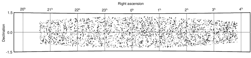
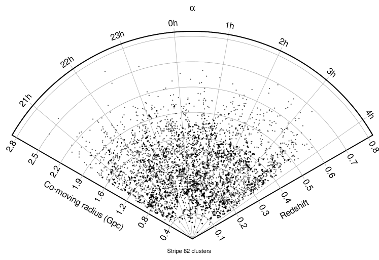
Figure 1: Sky and redshift distribution of clusters detected in Stripe 82. The top panel shows the angular distribution (Aitoff projection) and the lower cone plot indicates the redshift distribution over the full right ascension range of the Stripe, projected in $\sim$2.5 degrees of declination. Larger points indicate BCGs with spectroscopic measurements (we describe redshift estimation of clusters in §§3.3.1). We comfortably detect clusters out to $z\sim 0.6$, with a handful of systems potentially detected at higher redshifts. Beyond this, the 4000Å break moves into the near-IR, and selection using the Sloan optical bands alone becomes inefficient.

3 Detection of clusters in the Sloan Digital Sky Survey Equatorial Stripe 82

3.1 Data selection

We used the SDSS Catalog Archive Server (CAS) to extract griz ‘modelMag’ photometry from the PhotoObj table for all galaxies in the Stripe 82 co-add. We enforce a magnitude limiting range: $14<r\leq 24$ mag, and to eliminate stellar contamination we stipulate an additional minimum offset between the point-spread function fit magnitude and model magnitude: $(r_{\rm PSF}-r_{\rm model})>0.05$ mag. All photometry is corrected for Galactic extinction using the relevant ‘extinction’ table value (Schlegel et al. 1998). To remove overly de-blended, saturated and sources near frame edges, we also make use of the CAS fPhotoFlags parameter. We require all of the following to hold:

• BINNED1 or BINNED2 or BINNED4 $>$ 0

• BLENDED or NODEBLEND or CHILD !$=$ BLENDED

• EDGE or SATURATED $=$ 0

There are a total of 11,154,087 galaxies in the catalogue, and for convenience we split them into 0.2^h sectors in right ascension, overlapping by $\sim$3^m. For every galaxy, we determine whether a spectroscopic redshift is available from either the SDSS Data Release 7 (DR7), 2dF–SDSS LRG and QSO (2SLAQ; Croom et al. 2009) or WiggleZ Data Release 1 (Drinkwater et al. 2010). If no spectroscopic redshift is available, we ingest DR7 photometric redshifts (Abazajian et al. 2009). We discuss the photometric redshifts in further detail in §3.3.1.

3.2 Cluster detection

To elaborate on the colour scanning technique described in §2.2, we apply the Voronoi tessellation after selecting galaxies in narrow ‘slices’ of colour in the $(g-r)$, $(r-i)$ and $(i-z)$ bands. Each slice is defined by a linear strip in colour-magnitude space, which can be normalised in colour (the normalisation is defined as the colour at 20th magnitude), and has a gradient and width. Although this filtering could be adapted or refined in several ways (for example, allowing the gradient of the slice to vary), in this catalogue we have chosen simply to apply a filter that fixes the width and slope for slices in $(g-r)$, $(r-i)$ and $(i-z)$. We assume that the slope of the red-sequence (i.e. where we expect the contrast of a cluster against the background will be maximised in a colour-slice) is also constant with redshift. This method of exploiting the red-sequence to detect clusters of galaxies was pioneered by Gladders & Yee (2000).

To fix the slope and width of the slices, we turn to the richest known cluster in Stripe 82: Abell 2631 (Abell et al. 1989; Böhringer et al. 2000). We linearly fit the colour-magnitude sequence in each set of filters for 126 cluster members. The slopes of the colour-magnitude relation in $(g-r)$, $(r-i)$ and $(i-z)$ are $-0.048$, $-0.017$ and $-0.023$ respectively. The width of each slice is increased until it selects 90% of the members (see Gladders et al. 1998), and in the same bands we find that the required widths are 0.152, 0.067 and 0.110 mag. We fixed the width of all slices to the largest of these, although some refinement or adaptation of this selection based on the detected clusters (e.g. a variable colour slope) could be made in future releases.

The width of the colour slices are in part motivated by the effect of photometric uncertainty: there will be a broadening in the sequence towards the faint end where the photometric errors inflate. In a slice of fixed width, the contamination of non-cluster members will increase, as will the rate of cluster members being randomly scattered out of the slice. To this end, we enforce additional magnitude limits in each band, set where the average 1$\sigma$ uncertainty in photometry becomes comparable to the width of our colour slice. We define this to be the magnitude at which 50% of galaxies in the slice have errors equivalent to the width of the slice. The limits in griz are 24.0, 23.5, 23.3 and 21.6 mag. These cuts cull the input catalogue to 3,346,380 galaxies.

The scan through colour-space is complete, in that we cover a parameter space that should contain all red-sequences that could be detected in the optical bands (i.e. before the 4000Å break is red-shifted out of this window). However, we do enforce a blue limit in $(g-r)$ which ensures we only select colours redder than the $z=0$ red-sequence, which we derive by extrapolating the equivalent colour at $r=20$ mag from the sequences of Coma and Virgo (Smith et al. 2009; Rines & Geller 2008). This corresponds to $(g-r)>0.47$ mag, which fixes the bluest limit for a red-sequence in the catalogue. Consecutive slices overlap, since in successive scans we increase the colour normalisation of the selection slice by 0.04 mag ($\sim$75% overlap) and so (by design) the same cluster may be detected more than once in different selections. Since the red-sequence has some scatter (both natural and from photometric errors), the contrast of the cluster against the background (after colour selection) will rise to a peak and then vanish as the colour slice moves red-wards of the ridge-line.

To improve the rejection of background and foreground sources, we filter the catalogue using slices in two filters simultaneously, and we use two combinations of filters to detect clusters over a wide redshift range: $\{(g-r),(r-i)\}$ and $\{(r-i),(i-z)\}$. To search for the highest redshift clusters we can possibly detect using this technique, we also make a scan in $(i-z)$ only. Multiple detections of the same cluster are identified if the red-sequences (fit by a straight line) are within the width of the photometric filter, or two clusters share the same BCG. To eliminate these multiple detections, we pick the ‘best’ cluster by selecting the cluster with the largest ‘reduced flux’: the sum of the flux of all members excluding the brightest three galaxies. Murphy, Geach & Bower (2010) describe in more detail the exact procedure for merging multiple cluster detections into a master catalogue.

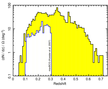
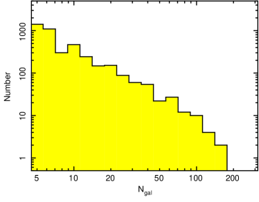
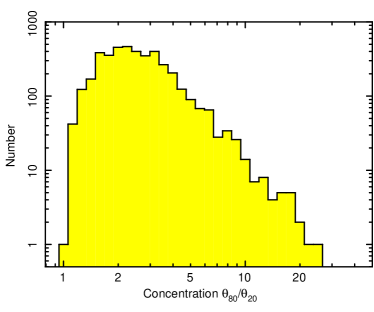
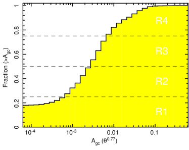
Figure 2: Vital statistics for the cluster catalogue. (top left) Redshift distribution for the Stripe 82 clusters, compared to the distribution of clusters identified using the maxBCG cluster detection algorithm (Koester et al. 2007a). Note that the maxBCG detector was not applied to the deeper multi-epoch photometry exploited in this work (see §3.3). The median redshift of clusters in the present catalogue is $\left<z\right>=0.32$. (top right) The distribution of cluster membership, where the minimum criteria for a cluster was 5 members. (bottom left) Concentration distribution, $C$, defined as the ratio of the radii of apertures containing 80% and 20% of the members. The concentration could be a useful parameter for the selection of sub-sets of the clusters. (bottom right) Richness classification (see §§3.3.2), based on quartile ranges of the distribution of $A_{\rm gc}$ – the estimated amplitude of the angular correlation function of galaxies in clusters. We define four simple classes of ascending richness: R1–R4.

3.3 Results

After catalogue cleaning and duplicate rejection, we detect a total of 4098 unique clusters with $\geq$5 members. We have applied the same algorithm to a mock catalogue generated from a semi-analytic prescription for galaxy formation (Bower et al. 2006) within a $\Lambda$CDM framework (the Millennium Simulation; Springel et al. 2005) to assess the efficacy of the algorithm where we can evaluate the completeness of the detection in terms of halo mass. This analysis suggests that at $z<0.4$ we are $>$68% complete for halos with mass $\log(M_{\rm h}/h^{-1}M_{\odot})\gtrsim 13.6$. This rises to $>$90% completeness for the most massive halos with $\log(M_{\rm h}/h^{-1}M_{\odot})\gtrsim 14$. Full details of this analysis, along with details of the mock catalogue are given in Murphy, Geach & Bower (2010).

It is important to note other cluster-finding efforts in the Stripe 82 region. The most significant cluster catalogue comparable to this is arguably the catalogue of clusters presented by Koester et al. (2007a) using the maxBCG algorithm (see Koester et al. 2007b). These clusters were detected across the full SDSS footprint, with 492 clusters in the Stripe 82 region. $\gtrsim$90% of clusters in the maxBCG catalogue (common to the Stripe 82 region) are detected in our catalogue. Direct comparison of the relative efficacy of the two algorithms is unfair, since the maxBCG catalogue was applied to the shallower SDSS photometry prior to the multi-epoch Stripe 82 co-added data. As a result, we are able to detect more clusters (including groups of fainter systems), out to higher redshifts than in Koester et al. (2007), as shown in Figure 2. Differences in the definition of a cluster also have an important role, especially at the low mass, or poor, end of the sample. First, restricting the current catalogue to $0.1\leq z\leq 0.3$ to better match the range of maxBCG we detect 1794 clusters and groups with $\geq$5 members. However, setting the minimum membership to $\geq$10 members, we find 504 systems, much more comparable to the maxBCG surface density.

Clearly then, the most important consideration that should be taken into account when comparing cluster catalogues is the selection function at the low mass end. The most massive clusters are likely to be detected easily even by very different techniques, since these will generally be very prominent in projection. However, differences in the completeness limit, minimum selection criteria and contamination rate can have a significant impact. As a test, we consider a mock catalogue of clusters generated from the Millennium Simulation, and populated with galaxies formed from the Bower et al. (2006) galform recipe. The number of halos detected increases by a factor $\sim$2 when between mass limits of 1–2$\times 10^{14}M_{\odot}$ (the estimated difference between the completeness limits of the maxBCG catalogue and ours). These considerations should be taken into account when comparing optically-selected cluster catalogues. Ideally, one would like to unify different catalogues that apply different search techniques. Cross-calibrating such a catalogue with independent mass estimates (such as weak lensing or X-ray luminosities), and tests on controlled mock-catalogues could provide a powerful resource for investigating the nature of the low-mass end of the cluster mass function.

In the following sub-sections we describe the main properties of our Stripe 82 cluster catalogue, including a description of our cluster redshift estimates, richness evaluation and expected false detection rate. A sky-plot of clusters detected in Stripe 82 is presented in Figure 1. Full details of the catalogue contents and information on accessibility are given in Appendix 1.

3.3.1 Redshift estimation

Red-sequence galaxies lend themselves well to photometric redshift ($z_{\rm p}$) estimation in the absence of spectroscopy: the prominent 4000Å break serves as a strong redshift discriminator in evolved galaxies. Approximately 32% of clusters in the catalogue have at least one member that has a spectroscopic redshift, while the remainder of members have a photometric redshift. Since the Stripe 82 multi-epoch data is deeper than the remainder of the SDSS DR7, we found some galaxies did not have pre-computed photometric redshifts. To this end, we used the code hyperz (Bolzonella et al. 2000) to estimate redshifts for any galaxy without an existing DR7 photometric redshift or spectroscopic redshift, exploiting the deeper ugriz Stripe 82 photometry.

The dispersion in $\delta z/(1+z)$ for $z^{\rm hyperz}_{\rm p}$ in a spectroscopically confirmed sample of 1549 galaxies in our cluster catalogue is 0.029, compared to 0.017 for the same galaxies when the photometric redshift is calculated with the DR7 algorithm (both figures calculated from the standard deviation in $\delta z/(1+z)$ after rejecting galaxies with $>$3$\sigma$ clipping). We attribute the higher precision in the DR7 photometric redshifts as due to the sophistication of the DR7 algorithm compared to our simple hyperz $\chi^{2}$ fits to a limited range of spectral templates. Thus, at the median redshift of the cluster sample, we expect photometric redshifts to be accurate to $\sim$5–9%.

Since we have several different redshifts for a given cluster, we can combine this information into a single redshift estimate for the cluster ensemble. We calculate a weighted median redshift for the system; spectroscopic redshifts are given a weighting of 4 (in effect, that galaxy is counted four times); photometric redshifts from the DR7 catalogue have a weighting of 2, and the hyperz calculated redshifts are given a weighting of unity. The lower weighting for the latter reflects the slightly poorer performance of these photometric redshifts compared to those from DR7 described above. A cone plot showing the redshift distribution of clusters in the Stripe is shown in Figure 1, and a histogram of the redshift distribution is shown in Figure 2. The median redshift of clusters in the survey is $\left<z\right>=0.32$, however the depth of the multi-epoch SDSS data in this region allows us to detect clusters comfortably out to $z\sim 0.5$, with a handful of systems detected at $z\gtrsim 0.6$.

3.3.2 Richness estimates

Often it is convenient to classify clusters according to their ‘richness’ – i.e. an observable parameter that correlates with the mass of the structure. In the absence of X-ray luminosities, velocity dispersions or accurate lens models of the underlying matter profile, we must rely on cruder methods of richness estimation that employ counting statistics to assess the significance of the density enhancement in the cluster compared to the field. Unfortunately, calibrating optical richness measurements to various mass estimates across different surveys is notoriously difficult, and so in this catalogue we have provided several (related) richness estimates based on aperture counts of cluster members corrected for field contamination. Moreover, the information provided in the cluster catalogue (Appendix 1) should be sufficient for the reader to either re-calculate a specific richness estimate, or re-calibrate our measured values to some other scale of their choice.

All of our richness estimates are based on the net counts of galaxies within an aperture of radius $\theta$ centred on the cluster centre (this is defined as the geometric mean centre of all members, or the position of the brightest cluster galaxy – again, the reader can adopt either position accordingly):

$$N_{\rm net}=N_{T}-N_{B}$$ (2)

where $N_{T}$ is the number of galaxies within the aperture, and $N_{B}$ is the number of background galaxies selected in an annulus centred on the cluster, with equivalent area to the $N_{T}$ selection aperture. Using an annulus instead of a scaled surface density for the full catalogue, although resulting in poorer number statistics, accounts for potential differences in photometric properties (seeing, local extinction, etc.) across different regions of the stripe. We have made no correction for the presence of bright star halos, or other cosmetic effects that might affect the counts in apertures. We adopt two values for $\theta$:

1. $\theta_{80}$ – the radius of an aperture containing 80% of the members

2. $\theta_{\rm 0.5Mpc}$ – the angular size of an aperture with projected physical size 0.5 Mpc

Similarly, the counts can be defined as either (a) all galaxies in the range $\left<m_{3},m_{3}+3\right>$, where $m_{3}$ is the magnitude of the third brightest cluster member, or (b) all galaxies in the photometric slice (described in §3.2) that the cluster was detected in.

There are issues with both (a) and (b) that introduce uncertainty to the richness calculation. We chose $m_{3}$ as a counting reference because it is purely empirical and can easily be derived from the catalogue without any additional assumptions about the cluster luminosity function. However, the scatter in $m_{3}$ will inflate both for low-number and high-$z$ clusters due to stochasticity, photometric uncertainties and projection effects. For example, in a redshift slice $0.2<z<0.3$, the standard deviation of $m_{3}$ measured for all clusters is strongly dependent on the number of galaxies assigned to the cluster, $N_{\rm gal}$. For clusters with $5\leq N_{\rm gal}\leq 10$ we find $\sigma(m_{3})=0.77$ mag, dropping to $\sigma(m_{3})=0.37$ mag for richer systems, $25\leq N_{\rm gal}\leq 35$. Similarly, in case (b), counting galaxies in a thin slice will result in uncertainty due to galaxies being scattered out of and into the slice – an issue that is also exacerbated for low-mass/faint systems.

Despite their limitations, from these basic statistics, we can derive higher order richness estimates. One commonly used measure is the $B_{\rm gc}$ statistic (Longair & Seldner 1979; Yee & Lopez-Cruz 2001) which has been shown to scale well with other more direct measurements of cluster mass (Yee & Ellingson 2003). This statistic is designed to estimate the amplitude of the spatial cross-correlation function for galaxies:

$$\xi(r)=B_{\rm gc}r^{-\gamma}.$$ (3)

To calculate $B_{\rm gc}$ requires a de-projection of the amplitude of the angular correlation function into 3D space, and this is estimated by:

$$B_{\rm gc}=\frac{\rho_{g}A_{\rm gc}}{\Phi(m_{l},z)I_{\gamma}}d_{\theta}^{\gamma-3}$$ (4)

where $\rho_{\rm g}$ is the average surface density of galaxies in the field brighter than a limit $m_{l}$, $d_{\theta}$ is the angular diameter distance to the redshift of the cluster, $\gamma$ is the slope of the power-law in the correlation function (equation 2), and $A_{\rm gc}$ is the amplitude of the angular correlation function, estimated as:

$$A_{\rm gc}=\frac{N_{\rm net}}{N_{B}}\frac{3-\gamma}{2}\theta^{\gamma-1}.$$ (5)

Finally, the $B_{\rm gc}$ statistic is scaled by the luminosity function, integrated between the absolute magnitude of the second brightest cluster member, down to the luminosity corresponding to $m_{l}$ at the redshift of the cluster (note that $I_{\gamma}=3.78$ – an integration constant, and $\gamma=1.77$). The limiting magnitude is set as $m_{3}+3$, where $m_{3}$ is the third brightest member of the cluster. Both $B_{\rm gc}$ and $A_{\rm gc}$ for both variants of angular scale and photometric selection described above are provided in the cluster catalogue to be used at the reader’s discretion, but here we prefer the angular correlation function amplitude calculated for $\theta_{80}$ and galaxies selected in the set of photometric filters the cluster was detected in. Unlike $B_{\rm gc}$, here we require no scaling for luminosity function. Finally, note that all of these statistics are ultimately governed by Poisson noise in $N_{T}$ and $N_{B}$. Naturally, this leads to a break-down of the practicality of these richness statistics in low-member (group) systems, and so should only be taken as a guide.

In order to coarsely segregate the catalogue into richness bins, we define four classifications of richness: R1–R4. These classifications are simply the quartile ranges of the parameter $A_{\rm gc}$, calculated inside $\theta_{80}$ and for all galaxies within the detection slice. The cumulative histogram and ranges are given in Figure 2. Finally, taken with a richness estimate, the concentration of galaxies in cluster can also be a useful parameter to describe the morphology of the system. We define a simple dimensionless concentration parameter $C=(\theta_{\rm 80}/\theta_{\rm 20})$. Where $\theta_{\rm 20}$ and $\theta_{\rm 80}$ are the radii of a circular aperture containing 20% and 80% of the members respectively. We find a median concentration of $\left<C\right>\sim 2.4$ (Figure 2).

3.3.3 False detections and contamination

A more comprehensive analysis of the completeness, purity, expected stellar mass recovery, and other statistical measures of the performance of the algorithm making use of mock catalogues are outlined in Murphy, Geach & Bower (2010). However, here it is instructive to outline the most important statistic pertinent to the current catalogue: the expect false positive detection rate.

To evaluate the inclusion of ‘clusters’ by erroneous random associations of galaxies. To evaluate this, we take the original Stripe 82 catalogue of galaxies and randomly shuffle the colours of galaxies, keeping the positions the same. Keeping the positions of galaxies constant ensures we replicate the natural random angular clustering of galaxies on the sky, but the randomisation of the colours allows us to assess how often these random associations could be linked by our assumption that group and cluster galaxies will have very similar colours. We apply the algorithm in exactly the same manner as the main detection, and find a rate of false detections of 0.06 ‘clusters’ per square degree. The vast majority of these false detections are made up of associations of 5 or 6 galaxies, near the lower cut-off for what we consider a group. Thus, the rate of false detections caused by random associations in the final catalogue is expected to be small, $<$1%.

An important caveat is that there could be added contamination from other incorrect identifications; mainly this will involve (i) associations of ‘galaxies’ that are actually the fragmented halos around bright stars; (ii) heavily, uniformly reddened galaxies in regions of high Galactic extinction; (iii) associations of ‘galaxies’ from overly de-blended galaxies in the catalogue. We have been careful to try to minimise the inclusion of such systems in the original catalogue obtained from CAS, however it is possible that some level of contamination in the final cluster catalogue could remain. Therefore, while our survey was exhaustive over the entire Stripe 82 area, the reader should exercise caution by flagging clusters that were detected in, for example, the vicinity of bright stars.

Another important source of contamination and completeness is the issue of the erroneous merging of structures along the line of sight, close in redshift (and therefore colour) space that are not physically connected. The separation of these systems in our algorithm depends on the relative difference between the red-sequences compared to the width of the colour ‘slices’ the two systems were detected in. To investigate how this might affect our catalogue, we have artificially created systems that are aligned along the line of sight and have identical red sequences. The colour of one of the sequences is reddened until the detector resolves the clusters into a pair; this indicates the minimum separation in redshift space (assuming a simple stellar population model for the colour difference of the red galaxies) at which the clusters can be resolved. In all cases, the projected clusters can be resolved when the separation between the red-sequences is approximately half of the width of the colour slice (of order 0.1 mag, see §3.2). Structures along the line of sight that have colour sequences separated by less than this are grouped into a single system and will only be disentangled by follow-up spectroscopy which can determine the relative velocity offsets of potential merged systems.

On a related note, the discrimination of structures at the same redshift, but separated by some projected distance is also important. The choice of critical threshold for Voronoi cell area (§2.1) can result in ‘valleys’ in the surface density of galaxies that could potentially fragment clusters with large amounts of sub-structure (e.g. two dense cores connected by some lower density filamentary structure). Based on experiments with mock catalogues, we have attempted to optimise the algorithm such that the level of fragmentation does not over-split clusters, whilst maintaining acceptable levels of cluster ‘purity’, completeness, etc. Full details of these experiments can be found in a sister paper, Murphy, Geach & Bower (2010).

3.4 Quasar sight-line catalogue

A powerful observational technique is the exploitation of continuum-bright background sources to search for spectroscopic evidence of absorption of continuum light by intervening intergalactic/intracluster material. For example, Lopez et al. (2008) present a study of 442 cluster-quasar pairs (sight-lines) within the Red Sequence Cluster Survey (RCS; Gladders & Yee 2000, 2005) where the Mg ii $\lambda\lambda$2796,2803 doublet could be detected at $0.3<z<0.9$. The study of the distribution of the equivalent width of absorption-line systems within clusters could provide a means of studying environmental effects such as gas-stripping in dense environment. The potential identification of high-ionisation absorption-line systems in the X-ray and UV could also provide a window onto the warm-hot phase of the intergalactic medium.

The large number of quasars already catalogued in the SDSS provides us with the opportunity to identify further potential targets for future sight-line studies, and here we supply a simple supplementary catalogue of 18,295 QSO-cluster pairs that might be useful for this purpose. We have taken the catalogue of Veron et al. (2010) and identified all QSOs with $0.25<z<2$ and $V\leq 21$ mag within a projected radius of foreground clusters that corresponds to 3 proper Mpc at the cluster redshift. A sub-set of the catalogue is given in Appendix 1 as a guide for content, and the full catalogue is available online at www.physics.mcgill.ca/$\sim$jimgeach/stripe82.

4 Summary

We have presented a catalogue of 4098 photometrically detected galaxy clusters in the Sloan Digital Sky Survey ‘Stripe 82’ equatorial multi-epoch co-add, a $\sim$270 square degree strip with photometry $\sim$2 mags deeper than the general SDSS imaging survey. The clusters have a median redshift of $\left<z\right>=0.32$, and we can comfortably detect systems out to $z\sim 0.5$, although photometry in redder bands is required for the efficient detection of higher-redshift systems. In addition to the cluster catalogue, we provide a supplementary catalogue of 18,295 $V\leq 21$ mag background QSO sight-lines, all within a projected radius of 3 proper Mpc of foreground clusters in this catalogue. These QSOs are simply cross-matches between clusters and QSOs in the catalogue of Veron et al. (2010). The sight-line catalogue will be a useful resource for future follow-up spectroscopic studies whose goals are the study of (for example) absorption line systems in cluster environments.

This catalogue is publicly available, and will be maintained from http://www.physics.mccgill.ca/$\sim$jimgeach/stripe82. Full details on access and content of the catalogue given in the Appendix of this paper. Readers are encouraged to contact the authors for any further information or assistance with the catalogues. We expect to improve the catalogue in future releases, with follow-up imaging and spectroscopy, and refinements of the detection algorithm. A forthcoming publication will present a more extensive catalogue of galaxy clusters detected using the same technique using SDSS DR7 data across the full SDSS footprint.

Appendix: distribution of the catalogue

The cluster catalogue is available at http://www.physics.mcgill.ca/$\sim$jimgeach/stripe82.

We have chosen to distribute the full catalogue in Hierarchical Data Format (HDF, version 5). This format provides a natural way for us to release both the ‘top level’ cluster properties (co-ordinate, redshift, etc.) and a wide range of other information, including various richness classifications, and information for each of the constituent galaxies. However, for simple access, we also provide a simple FITS table with just the basic ‘top-level’ data in. In Table A1 we list and describe the HDF data structure of the cluster catalogue. Both HDF5 and FITS format catalogues products are available for download at the website listed above.

For the QSO sight-line supplementary catalogue, we provide a simple FITS standard file with information on the QSO itself (taken from Veron et al. 2010), and a link to the relevant cluster in the main catalogue; however for convenience, we also provide some basic data on the matching cluster in this catalogue. The contents of the sight-line catalogue is provided in Table A2, and the file is available also from the website.

Table 1: Contents and hierarchy description of the Stripe 82 cluster catalogue. The top level information is also available as a stand-alone FITS table.

Hierarchy	Description
Top level
/ClusterNNNNN/ID	Cluster identification number
/ClusterNNNNN/ra	Cluster right ascension (degrees, J2000)
/ClusterNNNNN/dec	Cluster declination (degrees, J2000)
/ClusterNNNNN/ra_bcg	BCG right ascension (degrees, J2000)
/ClusterNNNNN/dec_bcg	BCG declination (degrees, J2000)
/ClusterNNNNN/ngal	Number of galaxies assigned to cluster
/ClusterNNNNN/redshift	Cluster redshift
/ClusterNNNNN/redshift_code	Code describing composite average of galaxy redshifts
/ClusterNNNNN/theta80	Angular radius containing 80% of the members ($\theta_{80}$)
/ClusterNNNNN/concentration	$\theta_{80}/\theta_{20}$ concentration measurement
/ClusterNNNNN/Agc	Richness estimator $A_{\rm gc}$
Richness measurements
/ClusterNNNNN/Richness/Class	Richness class R1–R4
/ClusterNNNNN/Richness/R500/RedSequence/...	Measured within 0.5 Mpc using red-sequence selection
/ClusterNNNNN/Richness/R500/MagLim/...	Measured within 0.5 Mpc using magnitude limited selection
/ClusterNNNNN/Richness/Theta80/RedSequence/...	Measured within $\theta_{80}$ using red-sequence selection
/ClusterNNNNN/Richness/Theta80/MagLim/...	Measured within $\theta_{80}$ using magnitude limited selection
.../Nb	Number of background galaxies within aperture
.../Nnet	Net number of galaxies within aperture
.../Agc	Richness estimator $A_{\rm gc}$
.../Bgc	Richness estimator $B_{\rm gc}$
Galaxy member information
/ClusterNNNNN/Galaxies/GalaxyNNN/objID	Member galaxy SDSS Stripe 82 PhotObjID
/ClusterNNNNN/Galaxies/GalaxyNNN/DR7_objID	Member galaxy SDSS DR7 PhotObjID
/ClusterNNNNN/Galaxies/GalaxyNNN/ra	Member galaxy $N$ right ascension (degrees, J2000)
/ClusterNNNNN/Galaxies/GalaxyNNN/dec	Member galaxy $N$ declination (degrees, J2000)
/ClusterNNNNN/Galaxies/GalaxyNNN/specz	Member galaxy $N$ spectroscopic redshift
/ClusterNNNNN/Galaxies/GalaxyNNN/specz_source	Member galaxy $N$ spectroscopic redshift source
/ClusterNNNNN/Galaxies/GalaxyNNN/photoz	Member galaxy $N$ photometric redshift
/ClusterNNNNN/Galaxies/GalaxyNNN/photoz_source	Member galaxy $N$ photometric redshift source
/ClusterNNNNN/Galaxies/GalaxyNNN/u	Member galaxy $N$ $u$-band model mag
/ClusterNNNNN/Galaxies/GalaxyNNN/g	Member galaxy $N$ $g$-band model mag
/ClusterNNNNN/Galaxies/GalaxyNNN/r	Member galaxy $N$ $r$-band model mag
/ClusterNNNNN/Galaxies/GalaxyNNN/i	Member galaxy $N$ $i$-band model mag
/ClusterNNNNN/Galaxies/GalaxyNNN/z	Member galaxy $N$ $z$-band model mag

Table 2: Contents and brief sub-set of the supplementary QSO sight-line catalogue. QSO ID and information is taken from the catalogue of Veron et al. (2010). The cluster ID corresponds to the ID listed in Table A1, although the corresponding cluster coordinates and redshift are also listed in this table. Note that one cluster may have multiple sight-lines. The impact parameter of the QSO to the cluster co-ordinate is given in terms of angle ($\theta$) and distance at the cluster redshift ($R$).

QSO ID	Cluster ID	QSO $z$	QSO $\alpha$	QSO $\delta$	QSO $V$	$\theta$	$R$	Cluster $z$	Cluster $\alpha$	Cluster $\delta$
			(deg)	(deg)	(mag)	(deg)	(Mpc)		(deg)	(deg)
119625	3390832343296285895	1.534	309.36000	$-$0.346389	20.37	0.117	2.22	0.27	309.470087	$-$0.306428
165873	3390832343296285895	0.634	309.47875	$-$0.472500	20.26	0.166	3.16	0.27	309.470087	$-$0.306428
119731	2567712495232746752	0.397	310.47292	0.485833	18.72	0.246	3.04	0.17	310.715893	0.521082
119752	2567712495232746752	1.378	310.63167	0.744444	19.51	0.239	2.96	0.17	310.715893	0.521082
119775	2567712495232746752	1.001	310.78667	0.781667	19.71	0.270	3.35	0.17	310.715893	0.521082
119785	2567712495232746752	1.915	310.86667	0.635000	20.09	0.189	2.34	0.17	310.715893	0.521082
165896	2567712495232746752	0.317	310.91667	0.481389	18.92	0.205	2.54	0.17	310.715893	0.521082

References

- Author et al. (2011) Abazajian, K. N., et al. 2009, ApJS, 182, 543
- Author et al. (2011) Abell, G. O., Corwin, H. G., Jr., Olowin, R. P., 1989, ApJS, 70, 1
- Author et al. (2011) Bolzonella, M., Miralles, J.-M., Pelló, R., 2000, A&A, 363, 476
- Author et al. (2011) Böhringer et al. 2000, ApJS, 129, 435
- Author et al. (2011) Bower, R. G., Benson, A. J., Malbon, R., Helly, J. C., Frenk, C. S., Baugh, C. M., Cole, S., Lacey, C. G., 2006, MNRAS, 370, 645
- Author et al. (2011) Croom, S. M., et al., 2009, MNRAS, 392, 19
- Author et al. (2011) Drinkwater, M. J., et al. 2010, MNRAS, 401, 1429
- Author et al. (2011) Ebeling, H., Wiedenmann, G., 1993, PhRevE, 47, 704
- Author et al. (2011) Gladders, M. D., Yee, H. K. C., 2000, AJ, 120, 2148
- Author et al. (2011) Gladders, M. D., Yee, H. K. C., 2005, ApJS, 157, 1
- Author et al. (2011) Gladders, M. D., Yee, H. K. C., Majumdar, S., Barrientos, L. F., Hoekstra, H., Hall, P. B., Infante, L., 2007, ApJ, 655, 128
- Author et al. (2011) Gladders, M. D., Lopez-Cruz, O., Yee, H. K. C., Kodama, T., 1998, ApJ, 501, 571
- Author et al. (2011) Gunn, J. E., et al., 1998, AJ, 116, 3040
- Author et al. (2011) Ho, S., Hirata, C., Padmanabhan, N., Seljak, U., Bahcall, N., 2008, PhRvD, 78, 3519
- Author et al. (2011) Kapferer, W., Kronberger, T., Ferrari, C., Riser, T., Schindler, S., 2008, MNRAS, 389, 1405
- Author et al. (2011) Kiang, T., 1966, ZA, 64, 433
- Author et al. (2011) Koester, B. P., et al. 2007a, ApJ, 660, 239
- Author et al. (2011) Koester, B. P., et al. 2007b, ApJ, 660, 221
- Author et al. (2011) Longair, M. S., Seldner, M., 1979, MNRAS, 189, 433
- Author et al. (2011) Lopez, S., et al, 2008, ApJ, 679, 1144
- Author et al. (2011) McCarthy, I. G., Frenk, C. S., Font, A. S., Lacey, C. G., Bower, R. G., Mitchell, N. L., Balogh, M. L., Theuns, T., 2008, MNRAS, 383, 593
- Author et al. (2011) Ramella, M., Boschin, W., Fadda, D., Nonino, M., 2001, A&A, 368, 776
- Author et al. (2011) Rines, K., Geller, M. J., 2008, AJ, 135, 1837
- Author et al. (2011) Rozo, E., et al. 2010, ApJ, 708, 645
- Author et al. (2011) Sawangwit, U., Shanks, T., Cannon, R. D., Croom, S. M., Ross, N. P., Wake, D. A., 2010, MNRAS, 402, 2228
- Author et al. (2011) Schlegel, D. J., Finkbeiner, D. P., Davis, M., 1998, ApJ, 500, 525
- Author et al. (2011) Smith, R. J., Lucey, J. R., Hudson, M. J., Allanson, S. P., Bridges, T. J., Hornschemeier, A. E., Marzke, R. O., Miller, N. A., 2009, Faint red galaxies in Coma cluster spectroscopy, VizieR On-line Data Catalog: J/MNRAS/392/1265
- Author et al. (2011) Springel, V., et al., 2005, Nature, 435, 629
- Author et al. (2011) van Breukelen, C., Clewley, L., 2009, MNRAS, 395, 1845
- Author et al. (2011) Veron-Cetty, M. P., Veron, P., 2010, Quasars and Active Galactic Nuclei (13th Ed.), VizieR Online Data Catalog
- Author et al. (2011) Yee, H. K. C., Ellingson, E., 2003, ApJ, 585, 215
- Author et al. (2011) York, D. G., et al. 2000, AJ, 120, 1579