Abstract

In computational biology, gene expression datasets are characterized by very few individual samples compared to a large number of measurements per sample. Thus, it is appealing to merge these datasets in order to increase the number of observations and diversify the data, allowing a more reliable selection of genes relevant to the biological problem. Besides, the increased size of a merged dataset facilitates its re-splitting into training and validation sets. This necessitates the introduction of the dataset as a random effect. In this context, extending a work of Lee et al. [2003], a method is proposed to select relevant variables among tens of thousands in a probit mixed regression model, considered as part of a larger hierarchical Bayesian model. Latent variables are used to identify subsets of selected variables and the grouping (or blocking) technique of Liu [1994] is combined with a Metropolis-within-Gibbs algorithm [Robert and Casella, 2004]. The method is applied to a merged dataset made of three individual gene expression datasets, in which tens of thousands of measurements are available for each of several hundred human breast cancer samples. Even for this large dataset comprised of around 20000 predictors, the method is shown to be efficient and feasible. As an illustration, it is used to select the most important genes that characterize the estrogen receptor status of patients with breast cancer.

Keywords: Bayesian variable selection, random effects, probit mixed regression model, grouping technique (or blocking technique), Metropolis-within-Gibbs algorithm.

1 Introduction

Selection of variables is a common problem in many scientific fields, and particularly in bioinformatics. Gene expression profiling analyses are notorious for generating a very large number of predictors compared to the number of observations. Microarray or high throughput sequencing technologies are important for finding genes that are implicated in biological processes including development, disease, and response to treatment, and it plays an important role in the current tendency towards personalized medicine. Identified genes or sequences can be used to classify future observations, influencing the treatment of patients. However, these experiments are expensive, and datasets have often no more than 100 specimens. The goal, therefore, is to advance a method allowing variable selection from merged microarray datasets, each of them presenting its own individual experimental bias.

Several model-based approaches have been developed to select variables. A well-known example is SVM (Support Vector Machine) with a recursive feature elimination of the genes (Guyon et al. [2002]). George and McCulloch [1993] and Chipman et al. [2001] developed Bayesian variable selection with the use of Gibbs sampling for linear models; a review of this type of selection is provided by O’Hara and Sillanpää. [2009]. Tadesse et al. [2005] proposed a Bayesian variable selection in a model-based clustering approach, using a multivariate Gaussian mixture model. Recently Bottolo and Richardson [2010] proposed an algorithm based upon Evolutionary Monte Carlo. Binary responses are often encountered in biostatistics studies, therefore probit or logistic models are implied. Bayesian variable selection methods have been proposed by Lee et al. [2003], Sha et al. [2004], Zhou et al. [2004b], Zhou et al. [2004c] and Yang and Song [2010] for probit regression, and by Zhou et al. [2004a], Chen and Dey [2003] and Tüchler [2008] for logistic regression. Extension to multi-category data has been done for the probit model in Albert and Chib [1993].

The motivation behind the variable selection method developed in this paper is to take the design of the study into account by using random effects in a mixed model. It is particularly suited to a merged microarray dataset design, and many such datasets are freely available from the NCBI GEO website [Edgar et al., 2002]. The increased size of a merged dataset may provide improved power, and facilitates its re-splitting into training and validation sets. In addition a merged set comprises more data diversity than an individual set, hence we can avoid bias due to a particular dataset as explained by various authors, see Cheng et al. [2010] and references therein. Among all the methods previously proposed for variable selection, that of Tüchler [2008] considered mixed models. However, her approach was specific for logistic models, and the method was applied to datasets with only few dozens predictors, whereas the aim of this paper is to select a few predictors among tens of thousands in a Bayesian framework. Recently Frühwirth-Schnatter and Wagner [2010] considered variable selection for random effects, but in this paper we are more interested by variable selection for the fixed effects, assuming that random effects are present.

The approach developed in this paper extends the approach of George and McCulloch [1993] and Lee et al. [2003]. George and McCulloch [1993] introduced latent variables to identify subsets of selected variables in a linear model. Then Lee et al. [2003] used these latent variables in a probit regression model, which is considered as part of a larger hierarchical Bayesian model. Our method extends the model used by Lee et al. [2003] by adding random effects. We are then confronted with several difficulties. One concerns the simulation of conditional distributions, since full conditional distributions cannot be directly simulated. A solution is to use the grouping (or blocking) technique of Liu [1994], and to combine Gibbs sampler and Metropolis-Hastings algorithms. Therefore the algorithm developed is a combination of the grouping method of Liu and the Metropolis-within-Gibbs algorithm [Robert and Casella, 2004]. A computational difficulty due to the large number of genes had also been overcome by imposing a fixed number of selected genes at each iteration of the algorithm. As a consequence the influence of the value chosen for the variable selection coefficient of our model is reduced. That represents an advantage, since the value of this coefficient can impact the results of other methods, see for instance Bottolo and Richardson [2010] who proposed to put a hyperprior distribution on this coefficient.

In this paper, Affymetrix microarray data are used, so predictors (genes) will be referred to as “probesets”, according to that technology. An Affymetrix U133plus2 microarray profiles all of the genes in the human genome, many of them more than once, using over 54000 gene-specific “probesets”. Our Bayesian variable selection method for probit mixed models is developed to select a few important probesets, among tens of thousands, which are indicative of the activity of the estrogen receptor gene in breast cancer. The severity of this common and deadly disease is directly related to estrogen receptor (ER) status, which is traditionally measured biochemically.
Three different breast cancer datasets were used, all with clinically defined ER status. One microarray experiment was done per patient, and ten of thousands of probesets were measured per experiment. The dataset is introduced as a random effect in the model, thus accounting for the different experimental conditions implicit in each set. The three merged datasets were split into training and validation sets, and the relevance of the selected probesets was checked by fitting a probit mixed model on the training set and predicting the ER status for the patients from the validation set and other independent sets available from the NCBI GEO website. The stability and the sensitivity of the algorithm were also checked by using the relative weighted consistency measure of Somol and Novovicova [2008].

The remainder of the paper is organized as follows. Section 2 describes the probit mixed model with latent variables. Section 3 gives the full conditional distributions necessary for the Gibbs sampling algorithm, outlines the algorithm and proposes a way to construct a classification rule using the selected probesets. Section 4 provides some experimental results on real datasets, on the relevance of selected probesets, and on the sensitivity and the stability of the method. Finally Section 5 discusses the method.

2 Probit mixed model for gene selection

2.1 The hierarchical model

Suppose that $n$ binary events are observed, denoted by the $Y_{i}$, $i=1,\ldots,n$. The set of potential regressors is of size $p$, with $p\gg n$. The goal is to select a subset of regressors related to the events $Y_{1},\ldots,Y_{n}$. The following probit mixed model is considered,

$$P(Y_{i}=1\mid U,\beta)=p_{i}=\Phi(X_{i}^{\prime}\beta+Z_{i}^{\prime}U),$$

where $\Phi$ stands for the standard Gaussian cumulative distribution function, and $X_{i}$ and $Z_{i}$ for the fixed and random effect regressors associated with the $i^{th}$ observation. The parameter $\beta$ corresponds to the fixed-effect coefficients and the parameter $U$ to the random-effect coefficients. $X$ and $Z$ are design matrices associated with the fixed and random effects.
Assuming that we have $K$ random effects, $U=(U_{1}^{\prime},\ldots,U_{K}^{\prime})^{\prime}$. Each $U_{l}$ is of size $q_{l}$, and $\sum_{l=1}^{K}q_{l}=q$. The size of $\beta$ is $p$.

Following Albert and Chib [1993] and Lee et al. [2003], a vector of latent variables $L$ is introduced. We write $L=(L_{1},\ldots,L_{n})$ and we assume that $L\mid U,\beta\sim\mathcal{N}_{n}(X\beta+ZU,I_{n})$ with $I_{n}$ the identity matrix. We then have

$$Y_{i}=\left\{\begin{array}[]{rl}1&\text{if }L_{i}>0\\ 0&\text{if }L_{i}<0,\end{array}\right.$$ (1)

To perform variable selection, a vector $\gamma$ of $p$ indicator variables is introduced:

$$\gamma_{j}=\left\{\begin{array}[]{rl}1&\text{if }\beta_{j}\neq 0,\quad\text{variable }j\text{ selected}\\ 0&\text{if }\beta_{j}=0,\quad\text{variable }j\text{ not selected}.\end{array}\right.$$

Given $\gamma$, $\beta_{\gamma}$ is the vector of all nonzero elements of $\beta$, and $X_{\gamma}$ is the matrix $X$ with only the columns corresponding to the elements of $\gamma$ that are equal to 1.

2.2 Prior distributions

To complete the hierarchical model, some prior assumptions have to be made on $U\mid D$, $\beta_{\gamma}\mid\gamma$, $\gamma$ and $D$, where $D$ is a covariance matrix of dimension $q$.

• If the data supports $\gamma_{j}=0$ over $\gamma_{j}=1$, then the $j^{th}$ variable will not be needed in the model and we can let $\beta_{j}=0$. We then focus on the prior distribution of the non null vector $\beta_{\gamma}$. Like Lee et al. [2003], we take the following conventional prior:

  $$\beta_{\gamma}\mid\gamma\sim\mathcal{N}_{d}(0,c(X_{\gamma}^{\prime}X_{\gamma})^{-1}),\qquad\textrm{with}\qquad d=\sum_{j=1}^{p}\gamma_{j},$$ (2)

  This prior corresponds to the g-prior of Zellner [1986], and $c$ is a positive scale factor specified by the user. Bottolo and Richardson [2010] called it the variable selection coefficient. Several authors discussed the choice of its value, see Chipman et al. [2001], George and Foster [2000], Clyde and George [2000] and Smith and Kohn [1997] among others. Raftery et al. [1997] used a similar form of prior. In our algorithm the value of $c$ will be fixed, but will not be too influent (see the discussion).

• The $\gamma_{j}$ are assumed to be independent Bernoulli variables, with

  $$P(\gamma_{j}=1)=\pi_{j},\qquad 0\leq\pi_{j}\leq 1.$$

  We do not want to use prior knowledge to favor any probesets, so we put $\quad\pi_{j}=\pi$, $\forall j=1,\ldots p$.

• The vector of coefficients associated with the random effects is assumed to be Gaussian and centered:

  $$U\mid D\sim\mathcal{N}_{q}(0,D).$$

  This definition allows three cases to be distinguished:
  

  General case: No structure is assumed for the variance-covariance matrix $D$, its prior distribution is an Inverse-Wishart $\mathcal{W}^{-1}(\Psi,m)$.
  

  Case of a block-diagonal matrix $D$: The different random effects are assumed independent. The vectors of coefficients associated with each random effect have Gaussian prior distributions:

  $$U_{l}\mid A_{l}\sim\mathcal{N}_{q_{l}}(0,A_{l}),\quad l=1,\ldots,K,$$

  where the $A_{l}$ are symmetric design matrices of dimension $q_{l}$. $D$ is a block-diagonal matrix denoted by $diag(A_{1},\ldots,A_{K})$. The prior distributions for each $A_{l}$ are Inverse-Wishart $\mathcal{W}^{-1}(\Psi,m)$.
  

  Case of a diagonal matrix $D$: $D=diag(A_{1},\ldots,A_{K})$ where $A_{l}=\sigma_{l}^{2}I_{q_{l}}$, $l=1,\ldots,K$ and $I_{q_{l}}$ the identity matrix. The prior distributions for the $\sigma_{l}^{2}$ are then Inverse Gamma $\mathcal{IG}(a,b)$ ($b$ denotes the scale).

3 Bayesian sampler for variable selection

3.1 The conditional distributions

The posterior distribution of $\gamma$ is of particular interest since it encapsulates the effectiveness of the different explanatory variables in explaining the variation in the responses $Y$. The number of possible explanatory variables is on the order of tens of thousands, so the number of possible $\gamma$-vectors is extremely large. The idea is to use a Gibbs sampling algorithm to explore this posterior distribution and search for high probability $\gamma$ values.

In order to use the classical Gibbs sampler, we must be able to simulate from all of the full conditional distributions (simplified by the hierarchical structure): $f(L\mid Y,\beta,U)$, $f(\beta\mid L,U,\gamma)$, $f(U\mid L,\beta,D)$, $f(\gamma\mid L,U,\beta)$ and $f(D\mid U)$.

• Full conditional distribution of $L$.

  $$L_{i}\mid\beta,U,Y_{i}=1 \sim \mathcal{N}(X_{i}^{\prime}\beta+Z_{i}^{\prime}U,1)\quad\textrm{left truncated at 0}$$

  $$L_{i}\mid\beta,U,Y_{i}=0 \sim \mathcal{N}(X_{i}^{\prime}\beta+Z_{i}^{\prime}U,1)\quad\textrm{right truncated at 0}.$$ (3)

• Full conditional distribution of $\beta$.
  Given $\gamma$, we know which elements of $\beta$ are not null. So we focus on the generation of the non null elements of $\beta_{\gamma}$. Letting $V_{\gamma}=\frac{c}{1+c}(X_{\gamma}^{\prime}X_{\gamma})^{-1}$, we have

  $$\beta_{\gamma}\mid L,U,\gamma \sim \mathcal{N}_{d}(V_{\gamma}X_{\gamma}^{\prime}(L-ZU),V_{\gamma})\qquad\textrm{with}\qquad d=\sum_{i=1}^{p}\gamma_{i}.$$ (4)

• Full conditional distribution of $U$.
  Defining $W=(Z^{\prime}Z+D^{-1})^{-1}$, we have

  $$U\mid L,\beta,D\sim\mathcal{N}_{q}(WZ^{\prime}(L-X\beta),W).$$ (5)

• Full conditional distributions of $\gamma$.

  $$f(\gamma\mid\beta_{\gamma},L,U) \propto (2\pi)^{-\frac{d}{2}}\exp\Big{[}-\frac{1}{2}\Big{(}-L^{\prime}X_{\gamma}\beta_{\gamma}-\beta_{\gamma}^{\prime}X_{\gamma}^{\prime}L+\beta_{\gamma}^{\prime}X_{\gamma}^{\prime}ZU+U^{\prime}Z^{\prime}X_{\gamma}\beta_{\gamma}+\beta_{\gamma}^{\prime}V_{\gamma}^{-1}\beta_{\gamma}\Big{)}\Big{]}$$ (6)

  $$\times\mid c(X_{\gamma}^{\prime}X_{\gamma})^{-1}\mid^{-\frac{1}{2}}\prod_{j=1}^{p}\pi_{j}^{\gamma_{j}}(1-\pi_{j})^{1-\gamma_{j}}.$$

• Full conditional distribution of $D$.
  General case: The full conditional distribution of $D$ is an Inverse-Wishart:

  $$D\mid U \sim \mathcal{W}^{-1}(UU^{\prime}+\Psi,m+1).$$ (7)

  Case of a block-diagonal matrix $D$: $D=diag(A_{1},\ldots,A_{K})$. The full conditional distribution of $A_{l}$ ($\forall l=1,\ldots,K$) is an Inverse-Wishart:

  $$A_{l}\mid U_{l} \sim \mathcal{W}^{-1}(U_{l}U_{l}^{\prime}+\Psi,m+1).$$ (8)

  Case of a diagonal matrix $D$: $D=diag(A_{1},\ldots,A_{K})$, and $\forall l=1,\ldots,K$, $A_{l}=\sigma_{l}^{2}I_{q_{l}}$. The full conditional distribution of $\sigma_{l}^{2}$ is an Inverse-Gamma:

  $$\sigma_{l}^{2}\mid U_{l} \sim \mathcal{IG}\Big{(}\frac{q_{l}}{2}+a,\big{(}\frac{1}{2}U_{l}^{\prime}U_{l}+b\big{)}\Big{)}.$$ (9)

3.2 Use of the grouping technique

The classical Gibbs sampler cannot be used because the full conditional distribution of $\gamma$ cannot be directly simulated (see (6)). However, this full conditional distribution can be simulated with a Metropolis-Hastings algorithm, and the complete algorithm would be a Metropolis-within-Gibbs algorithm. Roberts and Rosenthal [2006] have shown the Harris-recurrence of this algorithm, therefore its convergence is guaranteed. But even with a Metropolis-Hastings algorithm, the full conditional distribution of $\gamma$ is difficult to obtain, since it depends on the actual value of $\beta_{\gamma}$. Thus the acceptance rate for a candidate $\gamma^{*}$ in the Metropolis-Hastings algorithm will depend both on the actual $\gamma^{(t)}$ and $\beta_{\gamma^{(t)}}$, and on the proposed $\gamma^{*}$ and $\beta_{\gamma^{*}}$. The problem is that $\beta_{\gamma^{*}}$ is unknown.
To get around this problem, we combine the Metropolis-within-Gibbs algorithm with the grouping (or blocking) technique of Liu [1994]. The idea is to group the parameters $\beta_{\gamma}$ and $\gamma$, so we will be interested in the full conditional distribution of $(\beta_{\gamma},\gamma)\mid L,U$. This technique improves the algorithm and facilitates the convergence of the Markov chain, see Liu [1994] and van Dyk and Park [2008]. We note that the sampler obtained is then a special case of a Partial Collapsed Gibbs Sampler, see van Dyk and Park [2008].
As we have

$$f(\beta_{\gamma},\gamma\mid L,U)\propto f(\gamma\mid L,U)f(\beta_{\gamma}\mid\gamma,L,U),$$

we remark that simulating from the full conditional distribution $(\beta_{\gamma},\gamma)\mid L,U$ is equivalent to simulating $\gamma$ from its full conditional distribution integrated on $\beta_{\gamma}$, then simulating $\beta_{\gamma}$ from its full conditional distribution. The “integrated distribution” for $\gamma$ will not depend anymore on the nuisance parameter $\beta_{\gamma}$ and will be easily simulated by a Metropolis-Hastings algorithm.
In each iteration of the algorithm, we will take care to simulate $\gamma$ before $\beta{\gamma}$, to keep the dependence between $\beta{\gamma}$ and $\gamma$, as noted by van Dyk and Park [2008].

We use $f(L\mid\gamma,U)$ and the Bayes Theorem to get the integrated distribution of $\gamma\mid L,U$ (the target distribution):

$$f(\gamma\mid L,U) \propto (1+c)^{-\frac{\sum\gamma_{i}}{2}}\exp\Big{[}-\frac{1}{2}\Big{\{}(L-ZU)^{\prime}(L-ZU)$$

$$-\frac{c}{1+c}(L-ZU)^{\prime}X_{\gamma}(X_{\gamma}^{\prime}X_{\gamma})^{-1}X_{\gamma}^{\prime}(L-ZU)\Big{\}}\Big{]}\times\prod_{j=1}^{p}\pi_{j}^{\gamma_{j}}(1-\pi_{j})^{1-\gamma_{j}}.$$

3.3 The Metropolis-within-Gibbs sampler modified by the grouping technique

3.3.1 A Metropolis-Hastings step to simulate $\gamma$

At iteration $(i+1)$ of the Metropolis-Hastings algorithm, a candidate $\gamma^{*}$ will be proposed from $\gamma^{(i)}$. We want a symmetric transition kernel, to simplify the acceptance rate of the algorithm. The simplest way to have a symmetric transition kernel is to propose a $\gamma^{*}$ which corresponds to $\gamma^{(i)}$ in which $r$ components have been randomly changed (see Chipman et al. [2001] and George and McCulloch [1997]).

Given the target distribution (3.2), the acceptance rate $\rho$ is then:

$$\rho(\gamma^{(i)},\gamma^{*}) = min\Bigg{\{}\exp\Big{[}\frac{c}{2(1+c)}(L-ZU)^{\prime}\Big{(}X_{\gamma^{*}}(X_{\gamma^{*}}^{\prime}X_{\gamma^{*}})^{-1}X_{\gamma^{*}}^{\prime}-X_{\gamma^{(i)}}(X_{\gamma^{(i)}}^{\prime}X_{\gamma^{(i)}})^{-1}X_{\gamma^{(i)}}^{\prime}\Big{)}$$ (11)

$$\times(L-ZU)\Big{]}\times(1+c)^{\frac{\sum\big{(}\gamma_{j}^{(i)}-\gamma_{j}^{*}\big{)}}{2}}\times\Big{(}\frac{\pi}{1-\pi}\Big{)}^{\sum_{1}^{p}\big{(}\gamma_{j}^{*}-\gamma_{j}^{(i)}\big{)}},1\Bigg{\}}.$$

To facilitate the computation of the algorithm, the proposed $\gamma^{*}$ still corresponds to $\gamma^{(i)}$ for which $r$ components have been changed, but in such a way that the number of components whose values are 1 (and so the number of selected variables) is invariant. In so doing, $r/2$ components among the 1 values, and $r/2$ components among the 0 values are chosen at random and switched. There are several advantages to propose such a $\gamma^{*}$:

• In an iteration of the algorithm, if we have the number of variables selected $d$ higher than the number of observations $n$, the $X_{\gamma}^{\prime}X_{\gamma}$ matrix would be singular, and the prior distribution of $\beta_{\gamma}$ could not be defined as in (2). An advantage of fixing the number of variables to be selected at each iteration is that this number cannot increase during a run of the algorithm, and if $d$ is chosen lower than $n$ this case of non singularity of $X_{\gamma}^{\prime}X_{\gamma}$ is avoided.

• The acceptance rate is simplified, as we obtain $\sum\big{(}\gamma_{j}^{(t)}-\gamma_{j}^{*}\big{)}=0$.

• The choice of the prior value for the variable selection coefficient $c$ used in the prior distribution of $\beta$ is less influent (see the discussion).

Remark. In the method of Lee et al. [2003], the $\gamma$ vector is generated component by component at each iteration, while in our method a Metropolis-Hastings algorithm is used to generate it. There are two advantages to use a Metropolis-Hastings algorithm: it is computationally advantageous for a very large number of variables compared to a generation component by component, and it enables us to easily generate a $\gamma$ vector with an invariant number of components whose values are 1.

3.3.2 The sampler

The Metropolis-within-Gibbs sampler modified by the grouping technique of Liu generates a sequence:

$$\gamma^{(1)},\beta_{\gamma}^{(1)},D^{(1)},L^{(1)},U^{(1)},\ldots\ldots,\gamma^{(b+m)},\beta_{\gamma}^{(b+m)},D^{(b+m)},L^{(b+m)},U^{(b+m)}.$$

The sequence of the $\gamma^{(t)}$, which is of interest for the variable selection problem, is embedded in this ”Gibbs sequence”. To generate it, at each iteration $\gamma$ is simulated from its integrated distribution and $\beta_{\gamma},L,U$ and $D$ are simulated from their full conditional distributions.

Algorithm:
Starting with initial values $\gamma^{(0)},\beta^{(0)},D^{(0)},L^{(0)},U^{(0)}$. At iteration $t+1$:

1. Simulate $\gamma^{(t+1)}$ from $f(\gamma\mid L^{(t)},U^{(t)})$ (see 3.2), using the Metropolis-Hasting (MH) step. The MH step begins with $\gamma^{(t)}$ as an initial value, and $k$ iterations are performed given $L^{(t)}$ and $U^{(t)}$ ($k$ arbitrarily fixed). At iteration $i+1$ of the MH step:

   1. Generate the $\gamma^{*}$ candidate, by randomly switching $r/2$ components among the 1 values, and $r/2$ components among the 0 values.

   2. Take

      $$\gamma^{(i+1)}=\left\{\begin{array}[]{rl}\gamma^{*}&\text{with probability}\qquad\rho(\gamma^{(i)},\gamma^{*})\qquad\text{see (\ref{acceptancerate})}\\ \gamma^{(i)}&\text{with probability}\qquad 1-\rho(\gamma^{(i)},\gamma^{*})\end{array}\right.$$

   $\gamma^{(t+1)}$ will be the $\gamma^{(k)}$ obtained at the $k^{th}$ iteration of the MH step.

2. Simulate $\beta_{\gamma}^{(t+1)}$ from $f(\beta_{\gamma}\mid L^{(t)},U^{(t)},\gamma^{(t+1)})$ (see (4)).

3. Simulate $D^{(t+1)}$ from $f(D\mid U^{(t)})$ (see (7), (8) or (9)).

4. Simulate $L^{(t+1)}$ from $f(L\mid Y,\beta^{(t+1)},U^{(t)})$ (see (• ‣ 3.1)).

5. $U^{(t+1)}$ from $f(U\mid L^{(t+1)},\beta^{(t+1)},D^{(t+1)})$ (see (5)).

We use the fact that $X\beta=X_{\gamma}\beta_{\gamma}$ and that $\beta$ can be obtained from $\gamma$ and $\beta_{\gamma}$. The number of iterations is $b+m$, where $b$ corresponds to the burn-in period and $m$ to the observations from the posterior distributions.

In our application, we are not concerned by the strict convergence of the sampler. The aim is to find some relevant variables explaining the response, and to obtain good predictions. Hence we only need to do stability and sensitivity studies to check that the training set and the choices of the hyperparameters are not too influent, and we check the biological relevance of the variables selected.

3.3.3 The selected probesets

For selection of variables, the sequence $\{\gamma^{(t)}=(\gamma_{1}^{(t)},\ldots,\gamma_{p}^{(t)}),t=b+1,\ldots,b+m\}$ is used. The most relevant variables for the regression model are those which are supported by the data and prior information. Thus they are those corresponding to the $\gamma$ components with higher posterior probabilities, and can be identified as the $\gamma$ components that are most often equal to 1.

3.4 Classification and prediction

Once a set of relevant variables have been selected, it can be used to fit a probit mixed model in a classical way and to classify future observations. However, if more variables than necessary to fit a probit mixed model have been selected in the Bayesian selection step, a second selection has to be performed on them in order to build a reliable probit mixed model. This second selection is performed on the training set using standard selection tools like AIC, BIC, Bayes factors,…. The final probit mixed model can be tested on the validation set. Moreover, the variables selected in the Bayesian selection step can be used in other classification methods, such as Support Vector Machines (but random effects are not taken into account).

4 Experimental results

4.1 Application to the ER status of patients with breast cancer

4.1.1 Description of the datasets

Three different datasets were used: one private dataset from the Institut Paoli Calmettes (Marseille, France), consisting of 151 samples, and two datasets freely available from the NCBI GEO public website [Edgar et al., 2002]: accession numbers GSE2109 (310 samples) and GSE5460 (124 samples). Each dataset was treated for background noise and normalized with respect to a reference distribution by the RMA procedure [Irizarry et al., 2003]. Each dataset was split into a training set and a validation set having the same proportions of ER positive and ER negative observations. Then the three training datasets were merged on one side (497 patients) and the three validation sets were merged on the other side (88 patients).
For each patient, more than 54000 probesets were available. Two filters were applied on all of these probesets. Only the probesets sufficiently expressed so that they can be differentiated from noise and which could not be considered as invariant were kept, resulting in 19384 probesets. The goal was to select only a few probesets which are related to the ER status of the patients, by taking into account the different experimental conditions between the different merged datasets.

In this illustration, there are thousands of fixed regressors corresponding to the expression measurements of probesets, and only one random effect, which corresponds to the different datasets. $X_{ij}$ corresponds to the measurement of the expression level of the $j^{th}$ probeset for the $i^{th}$ patient, and $Z_{il}=1$ if the $i^{th}$ patient is from the $l^{th}$ dataset, 0 otherwise.

4.1.2 Prior settings for the algorithm

• Following the recommendations of Smith and Kohn [1997], a value of $c=50$ was chosen for the variable selection coefficient used in the prior distribution of $\beta$.

• Thirty probesets were selected at each iteration of the Gibbs sampler, when $\gamma$ is generated; $r=10$ of them were changed at each iteration of the Metropolis-Hastings step (5 zeros and 5 ones).

• The random effect corresponds to the dataset, and the three datasets are considered independent: they were generated in different countries, by different teams, using different equipments and different patients. Therefore the variance-covariance matrix of the random effect $D$ was a diagonal matrix $3\times 3$ with $A_{1}=\sigma_{1}^{2}I_{3}$. Gelman [2006] noted that an inverse-gamma prior should not be too non-informative, otherwise serious problems can arise. Given our data, we knew that $\sigma_{1}^{2}$ is probably not too high, and a $\mathcal{IG}(2,3)$ seemed reasonable for the prior distribution of $\sigma_{1}^{2}$.

• For the Metropolis-within-Gibbs sampler modified by the grouping technique, 60000 iterations were computed, among which 30000 were burn-in iterations. For the Metropolis-Hastings step in this sampler, 500 iterations were computed, and the simulated $\gamma$ was the one corresponding to the $500^{th}$ iteration.

4.1.3 Results and predictions

We performed a first selection of variables by selecting the top-rank probesets, those which have been selected the most often. A boxplot can help, see Figure 1. Forty probesets were selected at least once from the 30000 post-burn-in iterations of the simulated Markov Chain for $\gamma$. Twenty three probesets were selected in the 30000 iterations, and thirty were selected at least from 20000 iterations. There is a gap between probesets selected in more than 20000 iterations and others, so the first selection is made of these probesets selected at least in 20000 iterations.
A second selection was performed on the thirty probesets from the first selection, to build a reliable probit mixed model. This second selection was performed on the training set, using a stepwise selection (with AIC and BIC criteria) and the classification performance of the model on the validation set. Five probesets were kept: Affymetrix symbols 228241_at, 205862_at, 202376_at, 216222_s_at and 1568760_at. See Table 1 for the associated gene symbols and coefficients. The estimated random effects of this final model were reasonable: $-0.284$ for the dataset from the Institut Paoli Calmettes, $0.199$ for the GSE2109 dataset and $0.087$ for the GSE5460 dataset.

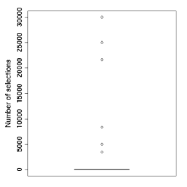
Figure 1: Boxplot of the number of selections of a probeset after the burn-in period, for the real datasets example. Forty probesets were selected at least once, all of the other probesets were never selected. A point represents a probeset (or several probesets if they have been selected the same number of times).

Probeset	gene	Coefficient	Pvalue
Intercept		-9.12074	1.92e-05
228241_at	AGR3	0.45046	1.12e-15
205862_at	GREB1	0.77639	4.18e-08
202376_at	SERPINA3	0.37965	0.000149
216222_s_at	MYO10	-0.63551	0.004967
1568760_at	MYH11	0.42742	0.050219

Table 1: Probesets selected in the final model and associated coefficients.

Using this 5-probeset model, two methods were used to predict the ER status of the patients in the validation set:

Using knowledge of the dataset to which each patient belonged and using the estimated random effects coefficients.

The estimated random effects coefficients are not used in order to mimic a real-life scenario of an experiment for a patient coming from an unknown dataset. The patients were predicted positive if their probability to be positive was higher than 0.5 and negative if it was lower than 0.5. The two methods gave us the same predictions, which were very good: a specificity of 1 and a sensitivity of 0.98 (1 wrong predictions among 88), see Figure 2.

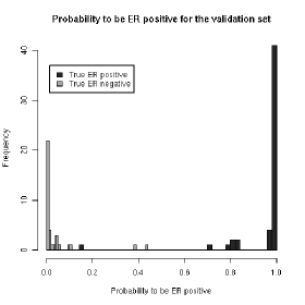
Figure 2: Histogram of probabilities to be ER positive given by the final model, for patients from the validation set.

Remark. In biomedical studies, when continuous variables are often reclassified as binary, it is common to define an “undetermined zone” of probabilities for which no prediction are given. Indeed, it is sometimes better than giving a wrong prediction, because these predictions imply treatments. Defining an “undetermined zone” between 10% and 90% probability of being positive, false predictions were eliminated, and 10 were considered undetermined (11.4%) (estimated random effects coefficients not used).

As a final test of our model, two more independent datasets were brought in from the NCBI GEO website: the GEO series GSE6532 and the GEO series GSE12763. The random effects associated with these datasets were entirely unknown, simulating an even more realistic case of prediction for a patient coming from an unknown dataset. Once again the results were very good : only 1 wrong prediction among 29 for the GSE12763 dataset, and no wrong predictions among 86 for the GSE6532 dataset.

4.2 Sensitivity and stability studies

The sensitivity and the stability of the algorithm were assessed by using the relative weighted consistency measure of Somol and Novovicova [2008], denoted by $CW_{rel}$. It is a measure evaluating how much subsets of selected variables for several runs overlap, and it shows the relative amount of randomness inherent in the concrete variable selection process. It takes values between 0 and 1, where 0 represents the outcome of completely random occurrence of variables in the selected subsets and 1 indicates the most stable variable selection outcome possible.
Stability is defined as sensitivity to variations in the training set. Referring to our breast cancer data set, 4000 probesets were randomly chosen from among the 19384 originally available. Since the aim here was only to check the sensitivity and stability of the method, these 4000 were not chosen in relation to the ER status.
Several runs of the algorithm were performed, and are reported in Table 2. Concerning the stability, the algorithm was run on three different training sets of 497 microarrays (among 585), using the same prior values for the hyperparameters. Concerning the sensitivity, the algorithm was run on the same training set with different values of $c$, different prior distributions for $\sigma_{1}^{2}$, different numbers of probesets to be selected at each iteration of the algorithm and different numbers of iterations. For the prior distributions for $\sigma_{1}^{2}$, we chose a $\mathcal{IG}(2,3)$ which seemed reasonable given our data, a $\mathcal{IG}(2,5)$ to have a prior favoring higher values compared to the first one, a $\mathcal{IG}(3,1)$ to favor lower values, and a $\mathcal{IG}(1,1)$ to have a non-informative prior without too small parameters to avoid problems, see Gelman [2006].

For each run, a reasonable number of probesets could be easily selected. Indeed, two to ten probesets were selected much more often than the others, see Figure 3 (two to four probesets were selected for most of the runs). Hence there is no need to perform a second selection, as in section 4.1.3. To compare the results of the different runs, the relative weighted consistency measure of Somol and Novovicova $CW_{rel}$ was used.

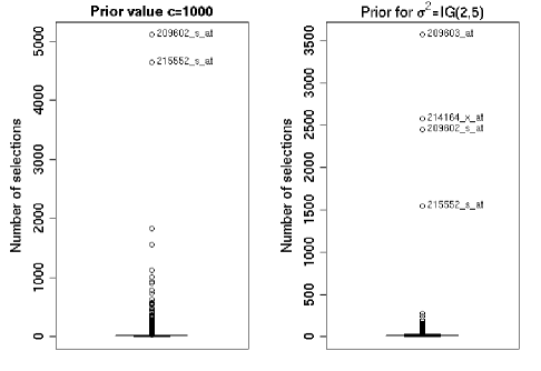
Figure 3: Boxplot of the number of selections of a probeset after the burn-in period, for two runs of the sensitivity analysis. A point represents a probeset (or several probesets if they have been selected the same number of times). The left boxplot corresponds to the run with $c=1000$: there is a gap between the two probesets selected in more than 4000 iterations and the others, hence we selected these two probesets. The right boxplot corresponds to the run with $\sigma_{1}^{2}\sim\mathcal{IG}(2,5)$: there is a gap between the four probesets selected in more than 1500 iterations and the others, hence we selected these four probesets.

		Value	Prior	Nb probesets to be	Nb probesets to be	Iterations	burn-in
Simu	Dataset	of	for	selected at each	changed at each	for the	for the	$CW_{rel}$
		$c$	$\sigma^{2}$	iteration of the GS	iteration of the MH	algo	algo
1	1
2	2
3	3	50	$IG(2,3)$	15	6	12000	6000	0.25
4		10
5		50
6		100
7	1	1000	$IG(2,3)$	15	6	12000	6000	0.375
8			$IG(2,3)$
9			$IG(1,1)$
10			$IG(1,1)$
11	1	50	$IG(2,5)$	15	6	12000	6000	0.292
12				15	6
13				5	2
14	1	50	$IG(2,3)$	30	10	12000	6000	0.5
15	1	50	$IG(2,3)$	15	6	30000	15000

Table 2: Parameters of the runs for the stability and sensitivity study and associated relative weighted consistency measure of Somol and Novovicova $CW_{rel}$. For the Metropolis-Hastings step, always 500 iterations are computed.

Using the results of the 15 runs together, $CW_{rel}=0.398$. Subsets of selected variables for the different runs overlapped: among the 15 runs the probesets 215552_s_at, 209603_at and 209602_s_at were kept in 12, 12 and 6 runs respectively. Apparently the prior for $\sigma^{2}$ ($CW_{rel}=0.292$) has more impact than the number of probesets to be selected at each iteration ($CW_{rel}=0.5$). We note that the number of probesets to be selected at each iteration of the algorithm and the number of iterations do not seem to modify the number of probesets more selected than the others during the run.

This was satisfying and the method appears relatively stable. First because the random selection of 4000 probesets carries a risk of destabilization of the results, since these 4000 are not necessarily those which are most indicative of ER status. Secondly, several probesets can represent the same gene, and different genes can be implied in the same biological pathway. Thus, it is possible that subsets of probesets are more similar than they appear, and therefore that $CW_{rel}$ is underestimated. For example, the probesets 209603_at and 209602_s_at mentioned above both represent the gene GATA3. Finally, these simulations indicate that there is not a parameter whose choice introduces more sensitivity than the others.

4.3 Comparison with other methods

We compared the performance of our method with the performances of other methods which do not take into account random effects: we considered the model of Lee et al. [2003] and Support Vector Machine with Recursive Feature Elimination of the variables, with linear or non linear kernels [Guyon et al., 2002]. We used simulated data: 200 observations of 1000 variables following a uniform distribution $\mathcal{U}_{[-5,5]}$ are generated. We assume that 5 variables and a random effect $U$ of size 4 explain a vector of binary variables $Y$ by a probit mixed model:

$$p_{i} = \Phi(X_{i}^{\prime}\beta+Z_{i}^{\prime}U),\qquad i=1,\ldots,200$$

$$Y_{i} \sim \mathcal{B}(p_{i}),\qquad i=1,\ldots,200$$

We took $\beta_{\gamma}=(-1,-1,1,1,2)$ and we assume that 50 observations are coming from each modality of the random effect. Different values of $U$ were used: $U1=(0,0,0,0)$, $U2=(-3,-2,2,3)$, $U3=(-5,-3,3,5)$, $U4=(-10,-5,5,10)$ and $U5=(-30,-10,10,30)$. This set of 200 observations was splitted into training and validation sets, each of them of size 100, with 25 observations coming from each modality of the random effect. For our method and the method of Lee et al. we took $c=50$, 5 probesets were selected at each iteration of the Gibbs sampler and $r=2$ of them were changed at each iteration of the Metropolis-Hastings step (1 zero and 1 one), $D$ was a diagonal matrix $3\times 3$ with $A_{1}=\sigma_{1}^{2}I_{3}$ and a prior $\mathcal{IG}(1,1)$ was chosen for $\sigma_{1}^{2}$, 500 iterations were performed for each Metropolis-Hastings step, and a total of 3000 and 5000 iterations were performed for the whole algorithm.
Concerning our method and the method of Lee et al. [2003], the top-ranked variables (variables selected more often than others, box-plots were used) were used to perform predictions on the validation set. The RFE-SVM method gave us directly sets of ”best variables” and associated models, and these models were used to perform the predictions. The results obtained are in Table 3.

Random effect	Our method		Lee et al. [2003] method		RFE-SVM
$U$	3000 iterations	5000 iterations	3000 iterations	5000 iterations	linear	non linear
$U1$	17	26	19	22	25	23
$U2$	19	21	19	19	20	26
$U3$	21	23	24	24	25	26
$U4$	19	19	35	35	29	31
$U5$	14	11	44	44	52	56

Table 3: Number of misclassifications on the validation set, for different methods and different random effects.

When there is no random effect or when the magnitude of the random effect is small, our method is comparable to the one of Lee et al., and the results of these two methods are better than or comparable with those obtained by RFE-SVM. But when the magnitude of the random effect is high, especially for $U4$ and $U5$, it appears that our method outperforms the method of Lee et al. and the RFE-SVM method.

5 Discussion

In this article we have developed an approach for Bayesian gene selection for a probit mixed model, as an extension of previous works by George and McCulloch [1993] and Lee et al. [2003]. An important contribution of our method is that it allows selection of variables in a mixed framework, taking into account the design of the data. It is particularly useful for gene selection, as it enables the use of merged datasets in order to introduce more observations and greater diversity. That may provide improved power, and we can avoid bias due to a particular dataset. The increased size of a merged dataset facilitates its re-splitting into training and validation sets, hence we do not need to evaluate the performance of a classification rule by a cross-validation procedure. It is advantageous compared to other methods which do not take into account random effects. Indeed, as these methods can use only one dataset which is usually of small size, they often need to perform leave-one-out-cross-validation, which can be time-consuming (see Lee et al. [2003], Yang and Song [2010], Sha et al. [2004], Zhou et al. [2004b] and Zhou et al. [2004c] for instance). On the contrary, if several datasets are merged then a separated training set can be used and the performance of a classifier can be directly obtained on it. Using simulations to make comparisons with other methods which do not take into account random effects, we showed that the proposed method is comparable to others when the magnitude of the random effects is low, but performs better than the others for classification when the magnitude of the random effects is high. This method should prove widely useful in microarray bioinformatics, since many diverse datasets are freely available on the Internet. But it can also be used for data obtained from high throughput sequencing technologies, which will probably be used a lot in few years. Indeed, the method can be applied when we have a matrix with $n<<p$ and an associated vector of random effects.

In practice, before running an analysis, one must decide how many variables will be selected at each iteration of the Gibbs sampler. We do not consider this to be a drawback, since in order to have a reliable selection, the number of probesets should be limited compared to the size of the training set. Besides, fixing the number of variables selected at each iteration is a computational advantage, as discussed in section 3.3.1. In particular, the singularity of the $X_{\gamma}^{\prime}X_{\gamma}$ matrix is avoided.
In addition, one must choose a value for the hyperparameter $c$ which is large enough to have a relatively non-informative prior. Only the simulations of $\beta_{\gamma}\mid L,U,\gamma$ and of $\gamma\mid L,U$ directly depend on $c$. Concerning $\beta_{\gamma}\mid L,U,\gamma$, we can see in (4) that the density is proportional to $c/(1+c)$, which is relatively close to 1 if $c$ is large. Concerning the density of $\gamma\mid L,U$ (see (3.2)), it depends on $c/(1+c)$ and on $(1+c)^{-\frac{\sum\gamma_{i}}{2}}$. The factor $(1+c)^{-\frac{\sum\gamma_{i}}{2}}$ does not play a role in the simulation of $\gamma$, because the number of variables to be selected at each iteration is fixed: this factor vanishes in the acceptance rate of the Metropolis-Hastings step of the algorithm. Therefore the value chosen should not be too influent, as long as it is large enough. We chose arbitrarily $c=50$, following Smith and Kohn’s (1997) recommendations. However different authors suggested different ranges, see Chipman et al. [2001], George and Foster [2000] and Clyde and George [2000] among others. For example Zhou et al. [2004b] and Zhou et al. [2004c] used $c=10$, and Lee et al. [2003] used $c=100$. However, it is possible to include another level in our Bayesian hierarchical model and to put a prior distribution on $c$. Zellner and Siow [1980] for instance proposed a mixture of g-priors and an inverse-gamma prior on $c$. Recently Bottolo and Richardson [2010] considered putting a hyperprior on $c$ and using a Metropolis-within-Gibbs with adaptive proposal for updating this coefficient. In our application this coefficient was held fixed for convenience, and good results were obtained. Besides the sensitivity study showed us that the method is not overly sensitive to the value chosen for $c$, as expected.
More generally, it appeared that the algorithm is fairly stable to variations in the training set, and is robust to prior value of any of the hyperparameters.

Convergence could not be verified because we did not have formal diagnostic tools to prove it, as the parameters vectors used in the proposed algorithm were not associated to the same variables from one iteration to the next. Besides, the different runs could have converged to a local mode of the posterior distribution of $\gamma$, and not to a global one. But the results obtained in the stability and sensitivity analyses were satisfactory, as different runs with different starting points and different prior hyperparameters selected broadly the same variables, which means that these different chains had basically the same behavior. From our experience, it appeared that having a total number of iterations equal to three times the size of the set of predictors is sufficient, the results were not significantly different when more iterations were performed.

The probesets selected by our method to characterize the estrogen receptor status enabled us to fit a model with good predictions. Moreover, three genes among the five used in the model were also selected using a Support Vector Machine method (twenty-four genes were selected by SVM), and another group of three among those five is known to be associated with estrogen receptor pathways and breast cancer: GREB1 [Nagaraja et al., 2006, Townson and O’Connell, 2006, Rae et al., 2005], SERPINA3 [Cimino et al., 2008] and MYH11 [Singh and Chaturvedi, 2009]. Therefore, it seems that the probesets selected by our method are quite biologically relevant.

The algorithm developed is efficient and feasible, even for very large datasets with around 20000 variables. Therefore this approach has a clear advantage over other selection methods which handle less variables or which do not take into account random effects. However, Bayesian variable selection is an active research area, and it would be interesting to combine our method with recent proposals. For instance by studying the performance of the method with other prior distributions for $\sigma^{2}$, like half-Cauchy or folded-noncentral-t distributions, see Gelman [2006]. Or by putting a prior distribution on $c$, like in Bottolo and Richardson [2010]. It would also be of interest to consider an alternative prior distribution for $\beta_{\gamma}$ to handle a non-invertible $X_{\gamma}^{\prime}X_{\gamma}$ (when $\gamma$ is itself singular or when $n<d$), by combining our approach with the concept of ridge regression (work in progress, Baragatti and Pommeret [2011]).

6 Acknowledgements

We would like to thank an Associate Editor and two anonymous reviewers for careful reading of the paper and constructive comments which have led to an improvement of the manuscript. We are grateful to Dr Daniel Birnbaum and Pr François Bertucci from the Département d’Oncologie Moléculaire of the Institut PAOLI CALMETTES (Marseille, France) for permission to use their data. We also thank Pr Denys Pommeret and Rebecca Tagett for useful discussions and comments.

References

- Albert and Chib [1993] J.H. Albert and S. Chib. Bayesian analysis of binary and polychotomous response data. Journal of the American Statistical Association, 88(422):669–679, 1993.
- Baragatti and Pommeret [2011] M.C. Baragatti and D. Pommeret. Ridge parameter for g-prior distribution in probit mixed models with collinearity. arxiv:1102.0470, 2011.
- Bottolo and Richardson [2010] L. Bottolo and S. Richardson. Evolutionary stochastic search for bayesian model exploration. Bayesian Analysis, 5(3):583–618, 2010.
- Chen and Dey [2003] M.H. Chen and D.K. Dey. Variable selection for multivariate logistic regression models. Journal of Statistical Planning and Inference, 111:37–55, 2003.
- Cheng et al. [2010] W.C. Cheng, M.L. Tsai, C.W. Chang, C.L. Huang, C.R. Chen, W.Y. Shu, Y.S. Lee, T.H W.ang, J.H. Hong, C.Y. Li, and I.C. Hsu. Microarray meta-analysis database (m2db): a uniformly pre-processed, quality controlled, and manually curated human clinical microarray database. BMC Bioinformatics, 11, 2010.
- Chipman et al. [2001] H. Chipman, E.I. George, and R.E. McCulloch. The practical implementation of bayesian model selection. In Model selection - IMS Lecture Notes. P. LAHIRI. Institute of Mathematical Statistics, 2001.
- Cimino et al. [2008] D. Cimino, L. Fuso, C. Sfiligoi, N. Biglia, R. Ponzone, F. Maggiorotto, G. Russo, L. Cicatiello, A. Weisz, D. Taverna, P. Sismondi, and M. De-Bortoli. Identification of new genes associated with breast cancer progression by gene expression analysis of predefined sets of neoplastic tissues. International Journal of Cancer, 123(6):1327–1338, 2008.
- Clyde and George [2000] M. Clyde and E.I. George. Flexible empirical bayes estimation for wavelets. Journal of the Royal Statistical Society B, 62(4):681–698, 2000. doi: 10.1111/1467-9868.00257.
- Edgar et al. [2002] R. Edgar, M. Domrachev, and A.E. Lash. Gene expression omnibus: NCBI gene expression and hybridization array data repository. Nucleic Acids Research, 30(1):207–210, 2002.
- Frühwirth-Schnatter and Wagner [2010] S. Frühwirth-Schnatter and H. Wagner. Bayesian Statistics 9., chapter Bayesian Variable Selection for Random Intercept Modeling of Gaussian and non-Gaussian Data. 2010.
- Gelman [2006] A. Gelman. Prior distributions for variance parameters in hierarchical models (comment on article by browne and draper). Bayesian Analysis, 1(3):515–534, 2006.
- George and Foster [2000] E.I. George and D.P. Foster. Calibration and empirical bayes variable selection. Biometrika, 87(4):731–747, 2000. doi: 10.1093/biomet/87.4.731.
- George and McCulloch [1993] E.I. George and R.E. McCulloch. Variable selection via gibbs sampling. Journal of the American Statistical Association, 88(423):881–889, 1993.
- George and McCulloch [1997] E.I. George and R.E. McCulloch. Approaches for bayesian variable selection. Statistica Sinica, 7:339–373, 1997.
- Guyon et al. [2002] I. Guyon, J. Weston, S. Barnhill, and V. Vapnik. Gene selection for cancer classification using support vector machines. Machine Learning, (46):389–422, 2002.
- Irizarry et al. [2003] R.A. Irizarry, B. Hobbs, F. Collin, Y.D. Beazer-Barclay, K.J. Antonellis, U. Scherf, and T.P. Speed. Exploration, normalization, and summaries of high density oligonucleotide array probe level data. Biostatistics, 4(2):249–264, 2003.
- Lee et al. [2003] K.E. Lee, N. Sha, E.R. Dougherty, M. Vannucci, and B.K. Mallick. Gene selection: a bayesian variable selection approach. Bioinformatics, 19(1):90–97, 2003.
- Liu [1994] J.S. Liu. The collapsed gibbs sampler in bayesian computations with application to a gene regulation problem. Journal of the American Statistical Association, 89(427):958–966, 1994.
- Nagaraja et al. [2006] G.M. Nagaraja, M. Othman, B.P. Fox, R. Alsaber, C.M. Pellegrino, Y. Zeng, R. Khanna, P. Tamburini, A. Swaroop, and R.P. Kandpal. Gene expression signatures and biomarkers of noninvasive and invasive breast cancer cells: comprehensive profiles by representational difference analysis, microarrays and proteomics. Oncogene, 25(16):2328–2338, 2006.
- O’Hara and Sillanpää. [2009] R.B. O’Hara and M.J. Sillanpää. A review of bayesian variable selection methods: What, how and which. Bayesian Analysis, 4(1):85–118, 2009.
- Rae et al. [2005] J.M. Rae, M.D. Johnson, J.O. Scheys, K.E. Cordero, J.M. Larios, and M.E. Lippman. GREB 1 is a critical regulator of hormone dependent breast cancer growth. Breast Cancer Research and Treatment, 92(2):141–149, 2005.
- Raftery et al. [1997] A.E. Raftery, D. Madigan, and J.A. Hoeting. Bayesian model averaging for linear regression models. Journal of the American Statistical Association, 92:179–191, 1997.
- Robert and Casella [2004] C. Robert and G. Casella. Monte Carlo statistical methods, second edition. Springer, 2004.
- Roberts and Rosenthal [2006] G.O. Roberts and J.S. Rosenthal. Harris recurrence of metropolis-within-gibbs and trans-dimensional markov chains. The Annals of Applied Probability, 16(4):2123–2139, 2006.
- Sha et al. [2004] N. Sha, M. Vannucci, M.G. Tadesse, P.J. Brown, I. Dragoni, N. Davies, T.C. Roberts, A. Contestabile, M. Salmon, C. Buckley, and F. Falciani. Bayesian variable selection in multinomial probit models to identify molecular signatures of disease stage. Biometrics, 60:812–819, 2004.
- Singh and Chaturvedi [2009] D. Singh and R. Chaturvedi. Recent patents on genes and gene sequences useful for developing breast cancer detection systems. Recent Patents on DNA and Gene Sequences, 3(2):139–147, 2009.
- Smith and Kohn [1997] M. Smith and R. Kohn. Non parametric regression using bayesian variable selection. Journal of Econometrics, 75:317–344, 1997.
- Somol and Novovicova [2008] P. Somol and J. Novovicova. Evaluating the stability of feature selectors that optimize feature subset cardinality. In N. da Vitora Lobo et al., editor, Lecture Notes in Computer Science, vol 5342, pages 956–966. Springer-Verlag Berlin Heidelberg, 2008.
- Tadesse et al. [2005] M.G. Tadesse, N. Sha, and M. Vannucci. Bayesian variable selection in clustering high-dimensional data. Journal of the American Statistical Association, 100:602–617, 2005.
- Townson and O’Connell [2006] S.M. Townson and P. O’Connell. Identification of estrogen receptor alpha variants in breast tumors: implications for predicting response to hormonal therapies. Journal of Surgical Oncology, 94(4):271–273, 2006.
- Tüchler [2008] R. Tüchler. Bayesian variable selection for logistic models using auxiliary mixture sampling. Journal of Computational and Graphical Statistics, 17(1):76–94, 2008.
- van Dyk and Park [2008] D.A. van Dyk and T. Park. Partially collapsed gibbs samplers: Theory and methods. Journal of the American Statistical Association, 103:790–796, 2008.
- Yang and Song [2010] A.J. Yang and X.Y Song. Bayesian variable selection for disease classification using gene expression data. Bioinformatics, 26(2):215–222, 2010.
- Zellner [1986] A. Zellner. Bayesian Inference and Decision Techniques – Essays in honour of Bruno De Finetti., chapter On assessing prior distributions and Bayesian regression analysis with g-prior distributions., pages 233–243. Amsterdam, 1986.
- Zellner and Siow [1980] A. Zellner and A. Siow. Posterior odds ratios for selected regression hypotheses. In Bayesian Statistics: Proceedings of the First International Meeting Held in Valencia, pages 585–603. University of Valencia Press, 1980.
- Zhou et al. [2004a] X. Zhou, K.Y. Liu, and S.T.C. Wong. Cancer classification and prediction using logistic regression with bayesian gene selection. Journal of Biomedical Informatics, 37:249–259, 2004a.
- Zhou et al. [2004b] X. Zhou, X. Wang, and E.R. Dougherty. A bayesian approach to non linear probit gene selection and classification. Journal of the Franklin Institute, (341):137–156, 2004b.
- Zhou et al. [2004c] X. Zhou, X. Wang, and E.R. Dougherty. Gene prediction using multinomial probit regression with bayesian gene selection. EURASIP Journal on Applied Signal Processing, (1):115–124, 2004c.