Orbit Determination with the two-body Integrals. II

Abstract

The first integrals of the Kepler problem are used to compute preliminary orbits starting from two short observed arcs of a celestial body, which may be obtained either by optical or radar observations. We write polynomial equations for this problem, that we can solve using the powerful tools of computational Algebra. An algorithm to decide if the linkage of two short arcs is successful, i.e. if they belong to the same observed body, is proposed and tested numerically. In this paper we continue the research started in [6], where the angular momentum and the energy integrals were used. A suitable component of the Laplace-Lenz vector in place of the energy turns out to be convenient, in fact the degree of the resulting system is reduced to less than half.

1 Introduction

We present a new method, based on the first integrals of the Kepler problem, to compute a finite set of preliminary orbits of a celestial body from two short arcs of observations. We assume that the body moves on a Keplerian orbit with a known center of attraction $O$, and is observed from a point $P$, whose motion is a known function of time. We deal with two different kinds of observations, optical and radar, and we make use of the related attributables (see [8], [12]).

In [6] the angular momentum and the energy integrals are used to solve the linkage problem for solar system bodies. This means to identify two attributables as related to the same observed object by computing (at least) one reliable orbit from the observations of both attributables. The equations of the problem are written in a polynomial form and the total degree of the system is 48. The use of these integrals for the linkage problem has been first proposed in [10], but without fully exploiting the algebraic character of the problem.

The algorithm presented in [6] has been used in [3] for the problem of correlation of space debris: here the authors have extended the method including the oblateness effect of the Earth.

In this paper we propose different equations for the same problem: in particular we use a suitable projection of the Laplace-Lenz vector in place of the energy. The advantage of this approach is that there are several cancellations and the total degree is 20.

The same equations can be written using different data, simply considering other quantities as unknowns: in Section 4 we deal with the case of an optical and a radar attributable. This case is peculiar because we end up with a univariate polynomial of degree 4. Thus this problem admits explicit solutions.

In both cases the solutions must fulfill compatibility conditions (as also shown in [6]), taking into account the other integrals of Kepler’s problem. To select the solutions we propose a different strategy, based on the attribution algorithm of a very short arc to a known orbit, see [8], [7].

The structure of the paper is the following. After introducing some definitions in Section 2, we study the linkage of two optical attributables in Section 3, while in Section 4 we consider the same problem with one optical and one radar attributable. The degenerate cases are shown in Section 5. Sections 6 and 7 are devoted to explain the computation of the covariance matrix for each orbit and the selection of the solutions. We conclude with a numerical test in Section 8.

2 Preliminaries

Let us fix an inertial reference frame, with the origin at the center of attraction $O$. The position ${\bf q}$ and velocity $\dot{\bf q}$ of the observer are known functions of time. We describe the position of the observed body as the vectorial sum

$${\bf r}={\bf q}+\rho\hat{\bf e}^{\rho}\,,$$ (1)

with $\rho$ the topocentric distance and $\hat{\bf e}^{\rho}$ the line of sight unit vector. We choose spherical coordinates $(\alpha,\delta,\rho)\in[-\pi,\pi)\times(-\pi/2,\pi/2)\times\mathbb{R}^{+}$, so that

$$\hat{\bf e}^{\rho}=(\cos\delta\cos\alpha,\cos\delta\sin\alpha,\sin\delta)\ .$$

A typical choice for $\alpha,\delta$ is right ascension and declination. Then we can write the velocity vector

$$\dot{\bf r}=\dot{\bf q}+\dot{\rho}\hat{\bf e}^{\rho}+\rho(\dot{\alpha}\cos\delta\hat{\bf e}^{\alpha}+\dot{\delta}\hat{\bf e}^{\delta})\,,\qquad\dot{\rho},\dot{\alpha},\dot{\delta}\in\mathbb{R},\rho\in\mathbb{R}^{+}\,,$$ (2)

where $\dot{\rho}$, $\rho\dot{\alpha}\cos\delta$, $\rho\dot{\delta}$ are the components of the velocity, relative to the observer in $P$, in the (positively oriented) orthonormal basis $\{\hat{\bf e}^{\rho},\hat{\bf e}^{\alpha},\hat{\bf e}^{\delta}\}$, with

$$\hat{\bf e}^{\alpha}=(\cos\delta)^{-1}\frac{\partial\hat{\bf e}^{\rho}}{\partial\alpha}\,,\hskip 28.45274pt\hat{\bf e}^{\delta}=\frac{\partial\hat{\bf e}^{\rho}}{\partial\delta}\ .$$

We recall the definitions of optical and radar attributables. From a short arc of optical observations of a moving body $(t_{i},\alpha_{i},\delta_{i})$ with $i=1\ldots m$, $m\geq 2$, it is possible to compute an optical attributable

$${\cal A}_{opt}=(\alpha,\delta,\dot{\alpha},\dot{\delta})\in[-\pi,\pi)\times(-\pi/2,\pi/2)\times\mathbb{R}^{2}\,,$$

representing the angular position and velocity of the body at a mean time $\bar{t}$ (see [8],[6]). In this case the radial distance and velocity $\rho,\dot{\rho}$ are completely undetermined and are the missing quantities to define an orbit for the body.

From a set of radar observations of a moving body $(t_{i},\alpha_{i},\delta_{i},\rho_{i})$, with $i=1\ldots m$, $m\geq 2$, it is possible to compute a radar attributable, i.e. a vector

$${{\cal A}}_{rad}=(\alpha,\delta,\rho,\dot{\rho})\in[-\pi,\pi)\times(-\pi/2,\pi/2)\times\mathbb{R}^{+}\times\mathbb{R}\,,$$

at time $\bar{t}$ (see [12]). Here $\dot{\alpha},\dot{\delta}$ are the unknowns needed to define an orbit.

We call attributable coordinates the vector $(\alpha,\delta,\dot{\alpha},\dot{\delta},\rho,\dot{\rho})$ representing the position and velocity of the body as seen from the observer at time $\bar{t}$.

3 Linking two optical attributables

Given two optical attributables ${\cal A}_{1},{\cal A}_{2}$ at epochs $\bar{t}_{1},\bar{t}_{2}$, we assume they belong to the same observed body and write 4 scalar algebraic equations for the topocentric distances $\rho_{1},\rho_{2}$ and the radial velocities $\dot{\rho}_{1},\dot{\rho}_{2}$ at the two epochs.

We use some of the algebraic integrals of the Kepler problem, i.e. the angular momentum ${\bf c}$, and the Laplace-Lenz vector ${\bf L}$. The expressions of these integrals as functions of the topocentric distance and radial velocity $\rho,\dot{\rho}$ are given below.

Angular momentum:

$${\bf c}(\rho,\dot{\rho})={\bf r}\times\dot{\bf r}={\bf D}\dot{\rho}+{\bf E}\rho^{2}+{\bf F}\rho+{\bf G}\,,$$

where

$$\begin{array}[]{l}{\bf D}={\bf q}\times\hat{\bf e}^{\rho}\,,\cr{\bf E}=\dot{\alpha}\cos\delta\hat{\bf e}^{\rho}\times\hat{\bf e}^{\alpha}+\dot{\delta}\hat{\bf e}^{\rho}\times\hat{\bf e}^{\delta}=\dot{\alpha}\cos\delta\hat{\bf e}^{\delta}-\dot{\delta}\hat{\bf e}^{\alpha}\,,\cr{\bf F}=\dot{\alpha}\cos\delta{\bf q}\times\hat{\bf e}^{\alpha}+\dot{\delta}{\bf q}\times\hat{\bf e}^{\delta}+\hat{\bf e}^{\rho}\times\dot{\bf q}\,,\cr{\bf G}={\bf q}\times\dot{\bf q}\ .\cr\end{array}$$

Laplace-Lenz’s vector:

$$\mu{\bf L}(\rho,\dot{\rho})=\dot{\bf r}\times{\bf c}-\mu\frac{{\bf r}}{|{\bf r}|}=\Bigl{(}|\dot{\bf r}|^{2}-\frac{\mu}{|{\bf r}|}\Bigr{)}{\bf r}-(\dot{\bf r}\cdot{\bf r})\dot{\bf r}\,,$$

where $\mu$ is a positive constant and

$$|{\bf r}| = (\rho^{2}+|{\bf q}|^{2}+2\rho{\bf q}\cdot\hat{\bf e}^{\rho})^{1/2}\,,$$

$$|\dot{\bf r}|^{2} = \dot{\rho}^{2}+(\dot{\alpha}^{2}\cos^{2}\delta+\dot{\delta}^{2})\rho^{2}+2\dot{\bf q}\cdot\hat{\bf e}^{\rho}\dot{\rho}+2\dot{\bf q}\cdot(\dot{\alpha}\cos\delta\hat{\bf e}^{\alpha}+\dot{\delta}\hat{\bf e}^{\delta})\rho+|\dot{\bf q}|^{2}\,,$$

$$\dot{\bf r}\cdot{\bf r} = \rho\dot{\rho}+{\bf q}\cdot\hat{\bf e}^{\rho}\dot{\rho}+(\dot{\bf q}\cdot\hat{\bf e}^{\rho}+{\bf q}\cdot\hat{\bf e}^{\alpha}\dot{\alpha}\cos\delta+{\bf q}\cdot\hat{\bf e}^{\delta}\dot{\delta})\rho+\dot{\bf q}\cdot{\bf q}\ .$$

Remark 1.

If $O$ corresponds to the center of the Sun, then we use interpolated values for ${\bf q},\dot{\bf q}$, as suggested by Poincaré [9]. If $O$ corresponds to the center of the Earth we do not apply this method.

These dynamical quantities give 6 scalar integrals of the motions: only 5 are mutually independent, in fact we have ${\bf L}\cdot{\bf c}=0$. Since we have 4 unknowns, generically we only need 4 scalar conservation laws to define a finite number of solutions. We select the conservation of the angular momentum vector and of a particular component of the Laplace-Lenz vector. The choice of the latter integral presents a substantial advantage with respect to the use of the energy, as in [6]: the difference between the two choices will be discussed later.

3.1 The polynomial equations

We use the notation above, with index 1 or 2 referring to the epoch. If ${\cal A}_{1}$, ${\cal A}_{2}$ correspond to the same observed object, then the angular momentum vectors at the two epochs must coincide:

$${\bf c}_{1}(\rho_{1},\dot{\rho}_{1})={\bf c}_{2}(\rho_{2},\dot{\rho}_{2})\ .$$ (3)

Equation (3) can be written as

$${\bf D}_{1}\dot{\rho}_{1}-{\bf D}_{2}\dot{\rho}_{2}={\bf J}(\rho_{1},\rho_{2})\,,$$ (4)

where

$${\bf J}(\rho_{1},\rho_{2})={\bf E}_{2}\rho_{2}^{2}-{\bf E}_{1}\rho_{1}^{2}+{\bf F}_{2}\rho_{2}-{\bf F}_{1}\rho_{1}+{\bf G}_{2}-{\bf G}_{1}\ .$$

Following [6] we eliminate the variables $\dot{\rho}_{1},\dot{\rho}_{2}$ and obtain the equation

$${\bf D}_{1}\times{\bf D}_{2}\cdot{\bf J}(\rho_{1},\rho_{2})=0\ .$$ (5)

We can write the left-hand side of (5) as

$$q(\rho_{1},\rho_{2})\stackrel{{\scriptstyle\rm def}}{{=}}q_{20}\rho_{1}^{2}+q_{10}\rho_{1}+q_{02}\rho_{2}^{2}+q_{01}\rho_{2}+q_{00}\,,$$ (6)

with

$$\begin{array}[]{l}q_{20}=-{\bf E}_{1}\cdot{\bf D}_{1}\times{\bf D}_{2}\,,\cr q_{10}=-{\bf F}_{1}\cdot{\bf D}_{1}\times{\bf D}_{2}\,,\cr\end{array}\hskip 28.45274pt\begin{array}[]{l}q_{02}={\bf E}_{2}\cdot{\bf D}_{1}\times{\bf D}_{2}\,,\cr q_{01}={\bf F}_{2}\cdot{\bf D}_{1}\times{\bf D}_{2}\,,\cr\end{array}$$

$$q_{00}=({\bf G}_{2}-{\bf G}_{1})\cdot{\bf D}_{1}\times{\bf D}_{2}\ .$$

The radial velocities are given by

$$\small\dot{\rho}_{1}(\rho_{1},\rho_{2})=\frac{({\bf J}\times{\bf D}_{2})\cdot({\bf D}_{1}\times{\bf D}_{2})}{|{\bf D}_{1}\times{\bf D}_{2}|^{2}}\,,\hskip 11.38092pt\dot{\rho}_{2}(\rho_{1},\rho_{2})=\frac{({\bf J}\times{\bf D}_{1})\cdot({\bf D}_{1}\times{\bf D}_{2})}{|{\bf D}_{1}\times{\bf D}_{2}|^{2}}\ .$$ (7)

Also the Laplace-Lenz vectors at the two epochs must coincide. We equate the projection of both vectors along ${\bf v}=\hat{\bf e}^{\rho}_{2}\times{\bf q}_{2}$:

$${\bf L}_{1}(\rho_{1},\dot{\rho}_{1})\cdot{\bf v}={\bf L}_{2}(\rho_{2},\dot{\rho}_{2})\cdot{\bf v}\ .$$ (8)

Actually the projection of ${\bf L}_{2}$ along ${\bf v}$ is particularly simple:

$$\mu{\bf L}_{2}\cdot{\bf v}=-(\dot{\bf r}_{2}\cdot{\bf r}_{2})(\dot{\bf r}_{2}\cdot{\bf v})\,,$$

thus (8) becomes

$$\Bigl{(}|\dot{\bf r}_{1}|^{2}-\frac{\mu}{|{\bf r}_{1}|}\Bigr{)}({\bf r}_{1}\cdot{\bf v})-(\dot{\bf r}_{1}\cdot{\bf r}_{1})(\dot{\bf r}_{1}\cdot{\bf v})=-(\dot{\bf r}_{2}\cdot{\bf r}_{2})(\dot{\bf r}_{2}\cdot{\bf v})\ .$$ (9)

After substituting (7), this is an algebraic equation in $\rho_{1},\rho_{2}$. Rearranging the terms in (9) and squaring we obtain

$$\small p(\rho_{1},\rho_{2})\stackrel{{\scriptstyle def}}{{=}}\mu^{2}({\bf r}_{1}\cdot{\bf v})^{2}-|{\bf r}_{1}|^{2}\left\{\left[|\dot{\bf r}_{1}|^{2}{\bf r}_{1}-(\dot{\bf r}_{1}\cdot{\bf r}_{1})\dot{\bf r}_{1}+(\dot{\bf r}_{2}\cdot{\bf r}_{2})\dot{\bf r}_{2}\right]\cdot{\bf v}\right\}^{2}=0\ .$$ (10)

This is a polynomial equation of degree 10 in $\rho_{1},\rho_{2}$: in fact, the projection

$$\begin{array}[]{ll}\dot{\bf r}_{2}\cdot{\bf v}&={\bf q}_{2}\cdot(\rho_{2}(\dot{\alpha}_{2}\cos\delta_{2}\hat{\bf e}^{\alpha}_{2}+\dot{\delta}_{2}\hat{\bf e}^{\delta}_{2})+\dot{\bf q}_{2})\times\hat{\bf e}^{\rho}_{2}=\cr&=\rho_{2}(-\dot{\alpha}_{2}\cos\delta_{2}{\bf q}_{2}\cdot\hat{\bf e}^{\delta}_{2}-\dot{\delta}_{2}{\bf q}_{2}\cdot\hat{\bf e}^{\alpha}_{2})+\hat{\bf e}^{\rho}_{2}\cdot{\bf q}_{2}\times\dot{\bf q}_{2}\cr\end{array}$$ (11)

does not depend on $\dot{\rho}_{2}$ and, in the difference $|\dot{\bf r}_{1}|^{2}{\bf r}_{1}-(\dot{\bf r}_{1}\cdot{\bf r}_{1})\dot{\bf r}_{1}$, the second degree term in $\dot{\rho}_{1}$ (i.e. $\dot{\rho}_{1}^{2}\rho_{1}\hat{\bf e}^{\rho}_{1}$) cancels out.

Therefore, to solve the linkage problem, we can consider the polynomial system

$$\left\{\begin{array}[]{l}p(\rho_{1},\rho_{2})=0\cr q(\rho_{1},\rho_{2})=0\cr\end{array}\right.\,,\hskip 28.45274pt\rho_{1},\rho_{2}>0\ .$$ (12)

with total degree 20. This shows the advantage of this method compared with the one in [6], which gives total degree 48.

3.2 Computation of the solutions

To compute the solutions of (12) we define an algorithm similar to the one in [4], [5], [6]. By grouping the monomials with the same power of $\rho_{2}$ we write

$$p(\rho_{1},\rho_{2})=\sum_{j=0}^{8}a_{j}(\rho_{1})\;\rho_{2}^{j}\,,\hskip 28.45274pt\mbox{where}$$ (13)

$$\deg(a_{j})=\left\{\begin{array}[]{lll}10&\mbox{ for }j=0&\cr 10-(j+1)&\mbox{ for }j=2k-1&\mbox{ with }k\geq 1\cr 10-j&\mbox{ for }j=2k&\mbox{ with }k\geq 1\cr\end{array}\right.$$

and

$$q(\rho_{1},\rho_{2})=b_{2}\;\rho_{2}^{2}+b_{1}\;\rho_{2}+b_{0}(\rho_{1})$$ (14)

for some univariate polynomial coefficients $a_{j},b_{0}$ and constants $b_{1},b_{2}$.

We consider the resultant $Res(\rho_{1})$ of $p,q$ with respect to $\rho_{2}$: it is generically a degree 20 polynomial defined as the determinant of the $10\times 10$ Sylvester matrix

$${\tt S}(\rho_{1})=\left(\begin{array}[]{ccccccc}a_{8}&0&b_{2}&0&\ldots&\ldots&0\cr a_{7}&a_{8}&b_{1}&b_{2}&0&\ldots&0\cr\vdots&\vdots&b_{0}&b_{1}&b_{2}&\ldots&\vdots\cr\vdots&\vdots&0&b_{0}&b_{1}&\ldots&\vdots\cr a_{0}&a_{1}&\vdots&\vdots&\vdots&b_{0}&b_{1}\cr 0&a_{0}&0&0&0&0&b_{0}\cr\end{array}\right)\ .$$ (15)

The positive real roots of $Res(\rho_{1})$ are the only possible values of $\rho_{1}$ for a solution $(\rho_{1},\rho_{2})$ of (12).

Remark 2.

The resultant of $p,q$ with respect to $\rho_{1}$ leads to compute determinants of $12\times 12$ matrices, thus the elimination of $\rho_{2}$ is more convenient. On the other hand, if we project the Laplace-Lenz vectors on $\hat{\bf e}^{\rho}_{1}\times{\bf q}_{1}$, it is better to eliminate $\rho_{1}$.

Following [6], we compute the coefficients of $Res(\rho_{1})$ by an evaluation-interpolation method based on the FFT, and then the roots $\rho_{1}(k)$ of $Res(\rho_{1})$ by the algorithm described in [1]. The computation of the preliminary orbits is concluded as follows:

• solve the equation $q(\rho_{1}(k),\rho_{2})=0$;

• discard spurious solutions, that is pairs $(\rho_{1},\rho_{2})$ solving (10) but not (9);

• compute the values of $\dot{\rho}_{1}(k),\dot{\rho}_{2}(k)$ by (7);

• write the corresponding orbital elements. The related epochs are $t_{i}={\bar{t}}_{i}-\rho_{i}(k)/c$, $i=1,2$ where $c$ is the velocity of light (aberration correction).

4 Linking radar and optical attributables

Assume we have a radar attributable ${\cal A}_{rad}=(\alpha,\delta,\rho,\dot{\rho})$ at epoch $\bar{t}$. We introduce the variables

$$\xi=\rho\dot{\alpha}\cos\delta\,,\hskip 28.45274pt\zeta=\rho\dot{\delta}$$

so that

$$\dot{\bf r} = \xi\hat{\bf e}^{\alpha}+\zeta\hat{\bf e}^{\delta}+(\dot{\rho}\hat{\bf e}^{\rho}+\dot{\bf q})\,,$$

$$|\dot{\bf r}|^{2} = \xi^{2}+\zeta^{2}+2\dot{\bf q}\cdot\hat{\bf e}^{\alpha}\xi+2\dot{\bf q}\cdot\hat{\bf e}^{\delta}\zeta+|\dot{\rho}\hat{\bf e}^{\rho}+\dot{\bf q}|^{2}\,,$$

$$\dot{\bf r}\cdot{\bf r} = {\bf q}\cdot\hat{\bf e}^{\alpha}\xi+{\bf q}\cdot\hat{\bf e}^{\delta}\zeta+(\dot{\rho}\hat{\bf e}^{\rho}+\dot{\bf q})\cdot{\bf r}\ .$$

The angular momentum as a function of $\xi,\zeta$ is

$$\mathbf{c}_{rad}(\xi,\zeta) = \mathbf{A}\xi+\mathbf{B}\zeta+\mathbf{C}\,,$$ (16)

where

$$\mathbf{A}={\bf r}\times\hat{\bf e}^{\alpha}\,,\qquad\mathbf{B}={\bf r}\times\hat{\bf e}^{\delta}\,,\qquad\mathbf{C}={\bf r}\times\dot{\bf q}+\dot{\rho}\,{\bf q}\times\hat{\bf e}^{\rho}\ .$$

Suppose we have a radar attributable ${\cal A}_{rad}$ at time $\bar{t}_{1}$ and an optical attributable ${\cal A}_{opt}$ at time $\bar{t}_{2}$. Equating the angular momentum vectors ${\bf c}_{rad}$ and ${\bf c}_{opt}$ at the two epochs we obtain a polynomial system of 3 equations in the 4 unknowns $\xi_{1},\zeta_{1},\rho_{2},\dot{\rho}_{2}$:

$${\bf A}_{1}\xi_{1}+{\bf B}_{1}\zeta_{1}+{\bf C}_{1}={\bf D}_{2}\dot{\rho}_{2}+{\bf E}_{2}\rho_{2}^{2}+{\bf F}_{2}\rho_{2}+{\bf G}_{2}\ .$$ (17)

The system is linear in $\xi_{1},\zeta_{1},\dot{\rho}_{2}$. By solving for these variables we obtain

$$\left\{\begin{array}[]{rcl}\xi_{1}(\rho_{2})&=&{\sf X}_{2}\rho_{2}^{2}+{\sf X}_{1}\rho_{2}+{\sf X}_{0}\cr\zeta_{1}(\rho_{2})&=&{\sf Z}_{2}\rho_{2}^{2}+{\sf Z}_{1}\rho_{2}+{\sf Z}_{0}\cr\dot{\rho}_{2}(\rho_{2})&=&{\sf R}_{2}\rho_{2}^{2}+{\sf R}_{1}\rho_{2}+{\sf R}_{0}\cr\end{array}\right.\ ,$$ (18)

where

$${\sf X}_{2}=\gamma\,{\bf E}_{2}\cdot{\bf B}_{1}\times{\bf D}_{2}\,, {\sf X}_{1}=\gamma\,{\bf F}_{2}\cdot{\bf B}_{1}\times{\bf D}_{2}\,, {\sf X}_{0}=\gamma\,({\bf G}_{2}-{\bf C}_{1})\cdot{\bf B}_{1}\times{\bf D}_{2}\,,$$

$${\sf Z}_{2}=-\gamma\,{\bf E}_{2}\cdot{\bf A}_{1}\times{\bf D}_{2}\,, {\sf Z}_{1}=-\gamma\,{\bf F}_{2}\cdot{\bf A}_{1}\times{\bf D}_{2}\,, {\sf Z}_{0}=-\gamma\,({\bf G}_{2}-{\bf C}_{1})\cdot{\bf A}_{1}\times{\bf D}_{2}\,,$$

$${\sf R}_{2}=-\gamma\,{\bf E}_{2}\cdot{\bf A}_{1}\times{\bf B}_{1}\,, {\sf R}_{1}=-\gamma\,{\bf F}_{2}\cdot{\bf A}_{1}\times{\bf B}_{1}\,, {\sf R}_{0}=-\gamma\,({\bf G}_{2}-{\bf C}_{1})\cdot{\bf A}_{1}\times{\bf B}_{1}\,,$$

and $\gamma=1/({\bf A}_{1}\cdot{\bf B}_{1}\times{\bf D}_{2})$.

Equating the expressions of the Laplace-Lenz vectors at the two epochs, and projecting along ${\bf v}=\hat{\bf e}^{\rho}_{2}\times{\bf q}_{2}$, yields

$$\mu[{\bf L}_{rad}(\xi_{1},\zeta_{1})-{\bf L}_{opt}(\rho_{2},\dot{\rho}_{2})]\cdot{\bf v}=$$

$$= \Bigl{[}\Bigl{(}|\dot{\bf r}_{1}|^{2}-\frac{\mu}{|{\bf r}_{1}|}\Bigr{)}{\bf r}_{1}-(\dot{\bf r}_{1}\cdot{\bf r}_{1})\dot{\bf r}_{1}\Bigr{]}\cdot{\bf v}+(\dot{\bf r}_{2}\cdot{\bf r}_{2})(\dot{\bf r}_{2}\cdot{\bf v})=0\ .$$

The term

$$\dot{\bf r}_{2}\cdot{\bf v} = \rho_{2}(-\dot{\alpha}_{2}\cos\delta_{2}{\bf q}_{2}\cdot\hat{\bf e}^{\delta}_{2}+\dot{\delta}_{2}{\bf q}_{2}\cdot\hat{\bf e}^{\alpha}_{2})+\hat{\bf e}^{\rho}_{2}\cdot{\bf q}_{2}\times\dot{\bf q}_{2}$$

does not depend on $\dot{\rho}_{2}$ and is linear in $\rho_{2}$ (cfr. with (11)). Thus, after substituting $\dot{\rho}_{2}=\dot{\rho}_{2}(\rho_{2})$, $\xi_{1}=\xi_{1}(\rho_{2}),\zeta_{1}=\zeta_{1}(\rho_{2})$ from (18), the terms $(\dot{\bf r}_{2}\cdot{\bf r}_{2})(\dot{\bf r}_{2}\cdot{\bf v})$ and $\bigl{[}|\dot{\bf r}_{1}|^{2}{\bf r}_{1}-(\dot{\bf r}_{1}\cdot{\bf r}_{1})\dot{\bf r}_{1}\bigr{]}\cdot{\bf v}$ are polynomials of degree 4 in $\rho_{2}$. We obtain a univariate polynomial equation with degree 4 in $\rho_{2}$, which admits explicit solutions. For each positive root $\rho_{2}(k)$ we can compute orbital elements at epochs $t_{1}=\bar{t}_{1}-\rho_{1}/c,t_{2}=\bar{t}_{2}-\rho_{2}(k)/c$ using (18).

5 Degenerate cases

We list the cases that make the equations of the linkage degenerate.

Optical case
The quadratic form (6) is completely degenerate if

$${\bf E}_{1}\cdot{\bf D}_{1}\times{\bf D}_{2}={\bf E}_{2}\cdot{\bf D}_{1}\times{\bf D}_{2}=0\ .$$

For a discussion on the geometric meaning of these conditions see [6]. Another degenerate case occurs if $\hat{\bf e}^{\rho}_{2}\times{\bf q}_{2}=0$. In the case of space debris this corresponds to a zenith observation.

Radar-Optical case
System (17) degenerates if

$${\bf A}_{1}\times{\bf B}_{1}\cdot{\bf D}_{2}=r_{1}^{\rho}({\bf r}_{1}\cdot{\bf D}_{2})=0\ .$$

This occurs when ${\bf r}_{1}\cdot\hat{\bf e}^{\rho}_{1}=0$, or ${\bf r}_{1}\times{\bf r}_{2}={\bf 0}$, or when $\hat{\bf e}^{\rho}_{2}$ is in the orbital plane (orthogonal to ${\bf r}_{1}\times{\bf r}_{2}$). Another degeneration occurs when $\hat{\bf e}^{\rho}_{2}\times{\bf q}_{2}=0$, as in the optical case.

6 Covariance of the solutions

Let ${\bf A}=({\cal A}_{1},{\cal A}_{2})$ be the vector of two optical attributables and $\Gamma_{{\bf A}}$ its covariance matrix. For each solution ${\bf Y}=(\rho_{1},\dot{\rho}_{1},\rho_{2},\dot{\rho}_{2})$ of the linkage problem

$$\left\{\begin{array}[]{l}{\bf c}_{1}(\rho_{1},\dot{\rho}_{1})={\bf c}_{2}(\rho_{2},\dot{\rho}_{2})\cr{\bf L}_{1}(\rho_{1},\dot{\rho}_{1})\cdot{\bf v}={\bf L}_{2}(\rho_{2},\dot{\rho}_{2})\cdot{\bf v}\cr\end{array}\right.\hskip 28.45274pt\rho_{1},\rho_{2}>0\,,$$ (19)

we can compute the Cartesian coordinates ${\cal E}_{car}^{(1)}$, ${\cal E}_{car}^{(2)}$ at epochs $t_{1},t_{2}$, and their covariance matrices $\Gamma_{car}^{(1)}$, $\Gamma_{car}^{(2)}$. We introduce the following notation:

• $\mathbf{E}_{car}=(\mathcal{E}_{car}^{(1)},\mathcal{E}_{car}^{(2)})$ is the 2 epochs Cartesian coordinates vector;

• $\mathbf{E}_{att}=(\mathcal{E}_{att}^{(1)},\mathcal{E}_{att}^{(2)})$, where

  $$\mathcal{E}_{att}^{(i)}=(\alpha_{i},\delta_{i},\dot{\alpha}_{i},\dot{\delta}_{i},\rho_{i},\dot{\rho}_{i})\,,\quad i=1,2\ .$$

Define the map $\bm{\Psi}:\mathbb{R}^{12}\to\mathbb{R}^{4}$ by

$$\mathbf{E}_{car}\stackrel{{\scriptstyle\bm{\Psi}}}{{\mapsto}}\left[\begin{array}[]{c}{\bf c}_{1}-{\bf c}_{2}\cr\mu({\bf L}_{1}-{\bf L}_{2})\cdot{\bf w}\end{array}\right]\ ,\hskip 28.45274pt{\bf w}={\bf r}_{2}\times{\bf q}_{2}\ .$$

Moreover, define $\mathcal{T}_{att}^{car}:\mathbf{E}_{att}\to\mathbf{E}_{car}$ by (1), (2) for both epochs, and consider the map $\bm{\Phi}=\bm{\Psi}\circ\mathcal{T}_{att}^{car}$. Then $\bm{\Phi}=\mathbf{0}$ is equivalent to (19).

The covariance matrix of the Cartesian coordinates at epoch $t_{1}$ is

$$\Gamma_{car}^{(1)}=\frac{\partial{\cal E}_{car}^{(1)}}{\partial{{\bf A}}}\Gamma_{{\bf A}}\left[\frac{\partial{\cal E}_{car}^{(1)}}{\partial{{\bf A}}}\right]^{T}\,,$$

with

$$\frac{\partial{\cal E}_{car}^{(1)}}{\partial{{\bf A}}}=\frac{\partial{\cal E}_{car}^{(1)}}{\partial{\cal E}_{att}^{(1)}}\frac{\partial{\cal E}_{att}^{(1)}}{\partial{{\bf A}}}\,,\hskip 28.45274pt\frac{\partial{\cal E}_{att}^{(1)}}{\partial{{\bf A}}}={\small\left[\begin{array}[]{c}\begin{array}[]{cc}I_{4}&O_{4}\cr\end{array}\cr\displaystyle\frac{\partial(\rho_{1},\dot{\rho}_{1})}{\partial{{\bf A}}}\cr\end{array}\right]}\ .$$

From the implicit function theorem

$$\frac{\partial{\bf Y}}{\partial{{\bf A}}}({\bf A})=-\left[\frac{\partial\bm{\Phi}}{\partial{\bf Y}}(\mathbf{E}_{att})\right]^{-1}\frac{\partial\bm{\Phi}}{\partial{{\bf A}}}(\mathbf{E}_{att})\,,$$

where

$$\frac{\partial\bm{\Phi}}{\partial{\bf Y}}=\left(\frac{\partial\bm{\Psi}}{\partial\mathbf{E}_{car}}\circ{\cal T}_{att}^{car}\right)\frac{\partial{\cal T}_{att}^{car}}{\partial{\bf Y}}\,,\hskip 28.45274pt\frac{\partial\bm{\Phi}}{\partial{{\bf A}}}=\left(\frac{\partial\bm{\Psi}}{\partial\mathbf{E}_{car}}\circ{\cal T}_{att}^{car}\right)\frac{\partial{\cal T}_{att}^{car}}{\partial{{\bf A}}}\ .$$

The matrices $\frac{\partial{\cal T}_{att}^{car}}{\partial{\bf Y}}$ and $\frac{\partial{\cal T}_{att}^{car}}{\partial{{\bf A}}}$ are respectively made by columns 5,6,11,12 and by columns 1,2,3,4,7,8,9,10 of $\frac{\partial\mathbf{E}_{car}}{\partial\mathbf{E}_{att}}$.

For a given vector ${\bf u}\in\mathbb{R}^{3}$ define the hat map

$$\mathbb{R}^{3}\ni(u_{1},u_{2},u_{3})={\bf u}\mapsto\widehat{\bf u}\stackrel{{\scriptstyle def}}{{=}}\left[\begin{array}[]{ccc}0&-u_{3}&u_{2}\cr u_{3}&0&-u_{1}\cr-u_{2}&u_{1}&0\cr\end{array}\right]\in so(3)\ .$$

Then we have, using $\hat{\bf u}^{T}=-\hat{\bf u}$,

$$\frac{\partial\bm{\Psi}}{\partial\mathbf{E}_{car}}=\left[\begin{array}[]{cccc}-\widehat{{\dot{\bf r}}_{1}}&\widehat{{{\bf r}}_{1}}&\widehat{{\dot{\bf r}}_{2}}&-\widehat{{{\bf r}}_{2}}\cr\stackrel{{\scriptstyle}}{{\displaystyle\frac{\partial\Delta_{\cal L}}{\partial{\bf r}_{1}}}}&\displaystyle\frac{\partial\Delta_{\cal L}}{\partial\dot{\bf r}_{1}}&\displaystyle\frac{\partial\Delta_{\cal L}}{\partial{\bf r}_{2}}&\displaystyle\frac{\partial\Delta_{\cal L}}{\partial\dot{\bf r}_{2}}\cr\end{array}\right]\,,$$

where

$$\frac{\partial\Delta_{\cal L}}{\partial{\bf r}_{1}}=\left(|\dot{\bf r}_{1}|^{2}-\mu\frac{1}{|{\bf r}_{1}|}\right){\bf w}^{T}+\mu\frac{({\bf r}_{1}\cdot{\bf w})}{|{\bf r}_{1}|^{3}}{\bf r}_{1}^{T}-(\dot{\bf r}_{1}\cdot{\bf w})\dot{\bf r}_{1}^{T}\,,$$

$$\frac{\partial\Delta_{\cal L}}{\partial\dot{\bf r}_{1}}=2({\bf r}_{1}\cdot{\bf w})\dot{\bf r}_{1}^{T}-(\dot{\bf r}_{1}\cdot{\bf w}){\bf r}_{1}^{T}-(\dot{\bf r}_{1}\cdot{\bf r}_{1}){\bf w}^{T}\,,$$

$$\frac{\partial\Delta_{\cal L}}{\partial{\bf r}_{2}}=\left(|\dot{\bf r}_{1}|^{2}-\frac{\mu}{|{\bf r}_{1}|}\right)[{\bf q}_{2}\times{\bf r}_{1}]^{T}-(\dot{\bf r}_{1}\cdot{\bf r}_{1})[{\bf q}_{2}\times\dot{\bf r}_{1}]^{T}+(\dot{\bf r}_{2}\cdot{\bf w})\dot{\bf r}_{2}^{T}+(\dot{\bf r}_{2}\cdot{\bf r}_{2})[{\bf q}_{2}\times\dot{\bf r}_{2}]^{T}\,,$$

$$\frac{\partial\Delta_{\cal L}}{\partial\dot{\bf r}_{2}}=(\dot{\bf r}_{2}\cdot{\bf w}){\bf r}_{2}^{T}+(\dot{\bf r}_{2}\cdot{\bf r}_{2}){\bf w}^{T}\ .$$

In the case of one radar and one optical attributable the covariance of the solutions can be computed in a similar way, with the following differences:

• the vector of the attributables is ${\bf A}=({\cal A}_{rad},{\cal A}_{opt})$,

• the vector of unknowns is ${\bf Y}=(\dot{\alpha}_{1},\dot{\delta}_{1},\rho_{2},\dot{\rho}_{2})$,

• the matrix of the derivatives of ${\cal E}_{att}^{(1)}$ with respect to ${\bf A}$ is

  $$\small\frac{\partial{\cal E}_{att}^{(1)}}{\partial{{\bf A}}}=\left[\begin{array}[]{c}\begin{array}[]{cccc}I_{2}&O_{2}&O_{2}&O_{2}\cr\end{array}\cr\displaystyle\frac{\partial(\dot{\alpha}_{1},\dot{\delta}_{1})}{\partial{{\bf A}}}\cr\begin{array}[]{cccc}O_{2}&I_{2}&O_{2}&O_{2}\cr\end{array}\cr\end{array}\right]\ ,$$

• The matrices $\frac{\partial{\cal T}_{att}^{car}}{\partial{\bf Y}}$ and $\frac{\partial{\cal T}_{att}^{car}}{\partial{{\bf A}}}$ are respectively made by columns 3,4,11,12 and by columns 1,2,5,6,7,8,9,10 of $\frac{\partial\mathbf{E}_{car}}{\partial\mathbf{E}_{att}}$.

7 Selecting solutions

The solutions of (19) are defined by using only four conservation laws. Thus ${\cal E}_{car}^{(1)}$, ${\cal E}_{car}^{(2)}$ may not correspond to the same orbit. We select the solutions of the linkage problem by means of the attribution algorithm [8], [7]. Here we recall briefly the procedure.

Let ${\cal E}_{1}$ be a set of orbital elements for the observed body at time $t_{1}$, with $6\times 6$ covariance matrix $\Gamma_{1}$. We can propagate the orbit with covariance to the epoch $t_{2}$ of an attributable ${\cal A}_{2}$, with a given $4\times 4$ covariance matrix $\Gamma_{{\cal A}_{2}}$, by the formula

$$\Gamma_{2}=\frac{\partial\Phi({\cal E}_{1},{\bar{t}}_{2})}{\partial{\cal E}_{1}}\Gamma_{1}\left[\frac{\partial\Phi({\cal E}_{1},{\bar{t}}_{2})}{\partial{\cal E}_{1}}\right]^{T}$$

where $\Phi({\cal E}_{1},t)$ is the integral flow of the Kepler problem. Then we can extract a predicted attributable ${\cal A}_{p}$, at time $\bar{t}_{2}$, with covariance matrix $\Gamma_{{\cal A}_{p}}$. Let $C_{{\cal A}_{p}}=(\Gamma_{{\cal A}_{p}})^{-1}$ and $C_{{\cal A}_{2}}=(\Gamma_{{\cal A}_{2}})^{-1}$. We define

$$C_{0}=C_{{\cal A}_{p}}+C_{{\cal A}_{2}}\,,\hskip 28.45274pt\Gamma_{0}=C_{0}^{-1}$$

The identification penalty is given by

$$\chi_{4}=({\cal A}_{2}-{\cal A}_{p})\cdot[C_{{\cal A}_{p}}-C_{{\cal A}_{p}}\Gamma_{0}C_{{\cal A}_{p}}]({\cal A}_{2}-{\cal A}_{p})\ .$$

If the value of $\chi_{4}$ is within a fixed threshold, we can accept the orbit ${\cal E}_{1}$.

Remark 3.

To select solutions we could also use compatibility conditions, as in [6]. In this case the conditions could be

$$({\bf L}_{1}-{\bf L}_{2})\cdot\hat{\bf e}^{\rho}_{2}=0\,,\hskip 28.45274pt\ell_{1}-\ell_{2}=n_{1}(t_{1}-t_{2})\ .$$ (20)

8 A test case

We present the results of a test of the method explained in Section 3 with the asteroid (99942) Apophis. We take two sets of 13 and 12 observations respectively with mean epochs $\bar{t}_{1}=53175.59$, $\bar{t}_{2}=53357.45$. After removing duplicate and spurious solutions we obtain

	$\rho_{1}$	$\rho_{2}$
1	0.78987	0.04345
2	1.13777	0.09569

Table 1: Solutions of the system (12) for ($(99942)$).

The two solutions gives respectively $\chi_{4}(1)=3230925.94$, $\chi_{4}(2)=2.29$, therefore we select the second one, with Keplerian elements (distances in AU, angles in degrees)

$$a=0.9230\,,\hskip 2.84544pte=0.189\,,\hskip 2.84544ptI=3.287\,,\hskip 2.84544pt\Omega=204.912\,,\hskip 2.84544pt\omega=124.778\,,\hskip 2.84544pt\ell=249.003$$

at epoch $t_{1}=53175.59$. We can compare the results with the known orbit propagated at epoch $t_{1}$:

$$a=0.9219\,,\hskip 2.84544pte=0.191\,,\hskip 2.84544ptI=3.333\,,\hskip 2.84544pt\Omega=204.575\,,\hskip 2.84544pt\omega=126.176\,,\hskip 2.84544pt\ell=247.500$$

In Figure 1, for the test case of (99942) Apophis, we show the intersections of the curves defined in this paper compared with the ones obtained by the conservation of the energy. In the four pictures the hyphened curve corresponds to equation (5). We also draw the curve defined by (9) on top left, and the one by (10), in polynomial form, on top right. The conservation of the energy defines the curve drawn on bottom left, its polynomial form (obtained by rearranging terms and squaring twice) defines the one on bottom right. The orbit determination method introduced in this paper, searching for the intersections shown on top right, is clearly convenient with respect to the method investigated in [6], related to figure on bottom right.

       

       

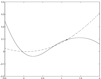
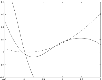
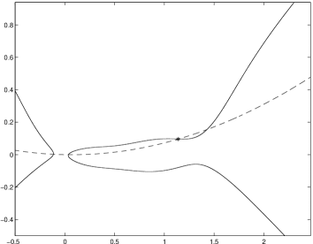
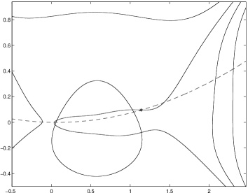
Figure 1: For the test case of (99942) Apophis, this figure shows the advantage of using equation (8) instead of the conservation of the energy $\mathcal{E}$. Top left: ${\bf c}$, ${\bf L}\cdot{\bf v}$ integrals. Top right: ${\bf c}$, ${\bf L}\cdot{\bf v}$ integrals, polynomial form. Bottom left: ${\bf c}$, $\mathcal{E}$ integrals. Bottom right: ${\bf c}$, $\mathcal{E}$ integrals, polynomial form.

9 Acknowledgments

We wish to thank A. Milani for his useful suggestions during the development of this work.

References

• [1] Bini, D. A.: 1997, Numerical computation of polynomial zeros by means of Aberth method, Numer. Algorithms 13, no. 3-4, 179–200.
• [2] Celletti, A., Negrini, P.: 1995, Non-integrability of the problem of motion around an oblate planet, CMDA 61, 253–260
• [3] Farnocchia, D., Tommei, G., Milani, A., Rossi, A.: 2010, Innovative methods of correlation and orbit determination for space debris, CMDA 107/1-2, 169–185
• [4] Gronchi, G. F.: 2002, On the stationary points of the squared distance function between two ellipses with a common focus, SIAM Journ. Sci. Comp. 24/1, 61–80
• [5] Gronchi, G. F.: 2005, An algebraic method to compute the critical points of the distance function between two Keplerian orbits, CMDA 93/1, 297–332
• [6] Gronchi, G. F., Dimare, L. and Milani, A.: 2010, Orbit determination with the two-body integrals, CMDA 107/3, 299–318
• [7] Milani, A., Gronchi, G. F.: 2009, Theory of Orbit Determination, Cambridge University Press
• [8] Milani, A., Sansaturio, M. E., Chesley, S. R.: 2001, The Asteroid Identification Problem IV: Attributions, Icarus 151, 150–159.
• [9] Poincaré, H.: 1906, Sur la détermination des orbites par la méthode de Laplace, Bulletin astronomique 23, 161–187.
• [10] Taff, L. G., Hall, D. L.: 1977, The use of angles and angular rates. I - Initial orbit determination, CMDA 16, 481–488
• [11] Taff, L. G., Hall, D. L.: 1980, The use of angles and angular rates. II - Multiple Observation Initial orbit determination, CMDA 21, 281–290
• [12] Tommei, G., Milani, A. and Rossi, A.: 2007, Orbit Determination of Space Debris: Admissible Regions, CMDA 97/4, 289–304