Entropy production in the non-equilibrium steady states of interacting many-body systems

Abstract

Entropy production is one of the most important characteristics of non-equilibrium steady states. We study here the steady-state entropy production, both at short times as well as in the long-time limit, of two important classes of non-equilibrium systems: transport systems and reaction-diffusion systems. The usefulness of the mean entropy production rate and of the large deviation function of the entropy production for characterizing non-equilibrium steady states of interacting many-body systems is discussed. We show that the large deviation function displays a kink-like feature at zero entropy production that is similar to that observed for a single particle driven along a periodic potential. This kink is a direct consequence of the detailed fluctuation theorem fulfilled by the probability distribution of the entropy production and is therefore a generic feature of the corresponding large deviation function.

I Introduction

The study of large deviation functions has been of increasing importance for the understanding of many-body systems. On the one hand large deviation functions form the basis of a modern approach to equilibrium statistical mechanics Ell85 ; Dem98 ; Tou09 , on the other hand they are increasingly recognized of being of fundamental interest for the characterization of non-equilibrium systems where they are sometimes considered to play a role similar to that played by the free energy at equilibrium. Important examples are given by the large deviations of the steady-state currents Ber07 ; Der07 in systems that are far from equilibrium.

Recently, Mehl et al. Meh08 extended the study of large deviation functions far from equilibrium to the steady-state entropy production. Studying a one-dimensional system composed of a single particle driven along a periodic potential, they reformulated the problem as a time-independent eigenvalue problem Leb99 and showed that for this system the large deviation function of the entropy production exhibits a kink at zero entropy production. Similar kinks in the large deviation function of the entropy production or in related large deviation functions of other quantities can also be found in a range of other systems Vis06 ; Tur07 ; Cle07 ; Lac08 ; Kum10 ; footnote1 . These are intriguing results that raise the important question whether the presence of this kink is a universal feature of systems with non-equilibrium steady states.

In this paper we study the entropy production in the steady states of different non-equilibrium interacting many-body systems. On the one hand we study the Partially Asymmetric Simple Exclusion Process (PASEP) Bly07 , a transport process in an open system where particles can enter or leave only at the system boundaries. On the other hand we investigate reaction-diffusion systems on a ring where the number of particles can change everywhere in the system due to reactions between the particles. Our main emphasis thereby is on the entropy production in the long-time limit where we study the large deviation function in the same way as done by Mehl et al. in their study of the single particle system. For all studied many-body systems we find a kink-like feature at zero entropy production, similar to what has been observed for the single particle system. We show that this kink is a generic feature in non-equilibrium systems obeying a detailed fluctuation theorem for the entropy production.

It is worth noting that large deviation functions of the current have been studied previously in some related systems. Studies of the Totally Asymmetric Simple Exclusion Process (TASEP) Der98 ; Der99 and of the Symmetric Simple Exclusion Process (SSEP) Kim95 ; Leb99 revealed a non-analytical behavior of the current large deviation function at the value 0 of the parameter that is canonically conjugated to the particle current. Using dynamical renormalization group techniques, it was later shown that the value of the corresponding exponent follows from the noise renormalization Lec07 . Very recently, Bodineau and Lagouge Bod10 studied the current large deviations in a driven dissipative lattice gas model with creation and annihilation processes, whereas Simon Sim10 investigated the large deviation function of the current for the Weakly Asymmetric Simple Exclusion Process on a ring.

Our paper is organized in the following way. In the next Section we introduce our models, before discussing in Section III our approaches for computing the entropy production at short times as well as the mean entropy production rate and the large deviation function for the entropy production in the long-time limit. Our results are presented and discussed in Section IV. Finally, Section V gives our conclusions.

II Models

In order to elucidate the entropy production in interacting many-body systems, we discuss in the following reaction-diffusion systems on a ring as well as open transport systems where particles move through a system that they can enter or leave only at its boundaries. In the past, due to the combination of their conceptual simplicity and highly non-trivial results, diffusion-limited reaction systems Hen08 ; Odo08 and simple exclusion processes Der98a ; Sch01 ; Gol06 have greatly contributed to our understanding of processes far from equilibrium. For the same reasons, these models are also the natural choices for our study of the entropy production in many-body systems.

As reaction-diffusion systems we consider simple cases where particles $A$ diffuse on a one-dimensional ring, under the condition that every lattice site can only be simply occupied. This diffusion process is mimicked by the hopping of a particle to an empty nearest neighbor site with rate $D$. In addition, we also allow for particle creation and annihilation. In the creation process a new particle can be created at an empty site with rate $h$, whereas in the annihilation process $n$ particles on $n$ connected sites are destroyed with rate $\lambda$, yielding $n$ empty sites. In the following we characterize our models by the number of particles involved in the annihilation process and call $M_{n}$ (with $n=2,3$) the model where $n$ particles are destroyed. As a variant, we also study the situation (we call the resulting model $M_{2^{\prime}}$) where in a two particles reaction only one particle is destroyed.

These models are the same as those studied in Dor09 ; Dor09b ; Dor10 in order to better understand steady-state and transient properties of reaction-diffusion systems. All these systems have non-equilibrium steady states. In addition, some or all reactions do not allow for a direct back-reaction, and microscopic reversibility is broken. However, as discussed in the next Section, the computation of the entropy production requires microscopic reversibility, i.e. for every reaction the direct back-reaction must be possible. For that reason we are adding to the reaction schemes the direct back-reactions of the reactions just described. Thus, any particle can be destroyed with rate $\varepsilon_{h}\,h$, with $0<\varepsilon_{h}<1$, irrespective of whether neighboring sites are occupied or not, and a reversing of the annihilation process yields the creation of particles with rate $\varepsilon_{\lambda}\,\lambda$, where $0<\varepsilon_{\lambda}<1$. It is important to note that even with these expanded reaction schemes our systems are still characterized by non-equilibrium steady states, as long as $\varepsilon_{h},\varepsilon_{\lambda}<1$. In the following we set $\varepsilon_{h}=\varepsilon_{\lambda}=\varepsilon$ and focus on the case $\varepsilon\ll 1$. For the convenience of the reader we summarize the different reaction schemes in Table 1.

$M_{2^{\prime}}$	$M_{n}$
$A+A\overset{\lambda}{\underset{\varepsilon_{\lambda}\lambda}{\rightleftarrows}}0+A$	$nA\overset{\lambda}{\underset{\varepsilon_{\lambda}\lambda}{\rightleftarrows}}n0$
$0\overset{h}{\underset{\varepsilon_{h}h}{\rightleftarrows}}A$	$0\overset{h}{\underset{\varepsilon_{h}h}{\rightleftarrows}}A$

Table 1: The different reaction schemes discussed in this work. The back-reactions are taking place with rates $\varepsilon_{h}h$ and $\varepsilon_{\lambda}\lambda$, with $0<\varepsilon_{h}<1$ and $0<\varepsilon_{\lambda}<1$.

As transport process we consider the Partially Asymmetric Simple Exclusion Process (PASEP) where every configuration is reversible. In the Total Asymmetric Simple Exclusion Process (TASEP) in an open one-dimensional system, particles that are fed into the system at, say, the left end with rate $\alpha$ can leave the system at the right end with rate $\beta$. Inside the system particles can only jump to a right neighboring site, provided that site is not occupied. Obviously, microscopic reversibility is always broken for this model. In the PASEP, however, particles can always jump in both directions, provided that the chosen site is empty, with the probability for a jump to the right being $p$, whereas the probability for a jump to the left is $1-p$. In addition, particles can exit the system at the left with probability $\varepsilon_{\alpha}\alpha$ (with $0<\varepsilon_{\alpha}<1$) and enter at the right with probability $\varepsilon_{\beta}\beta$ (with $0<\varepsilon_{\beta}<1$). It follows that microscopic reversibility is always fulfilled. In order to keep the number of parameters as small as possible, we set $\varepsilon_{\alpha}=\varepsilon_{\beta}=\varepsilon$, with $\varepsilon\ll 1$.

III Methods

Whereas our main focus in the following will be on the large deviation function of the steady-state entropy production in the long time limit, we will also briefly discuss the entropy production at short times.

Focusing on our lattice models, let us consider a path in configuration space $C_{0}\longrightarrow C_{1}\longrightarrow\cdots\longrightarrow C_{M-1}\longrightarrow C_{M}$ that starts at some configuration $C_{0}$ and ends at some configuration $C_{M}$ after $M$ diffusion or reaction steps. Every configuration $C_{i}$ is uniquely characterized by the occupation numbers (being 0 or 1) of all lattice sites. We will denote by $P_{S}(C_{i})$ the probability to find the configuration $C_{i}$ in the steady state. With every step $i$ leading from configuration $C_{i-1}$ to configuration $C_{i}$ we associate a time increment $\tau_{i}$ given by

$$\tau_{i}=\frac{1}{\sum_{j}\omega(C_{i-1}\longrightarrow\widetilde{C}_{j})}$$ (1)

where $\omega(C_{i-1}\longrightarrow\widetilde{C}_{j})$ is the rate with which we go from configuration $C_{i-1}$ to any other accessible configuration $\widetilde{C}_{j}$. The sum in the denominator is thereby a sum over all configurations $\widetilde{C}_{j}$ (including the configuration $C_{i}$ in which the system will be at step $i$) that can be reached from the configuration $C_{i-1}$ through diffusion or reaction. With that we can assign a total time

$$\tau=\sum\limits_{i=1}^{M}\tau_{i}$$ (2)

to our trajectory in configuration space.

Along the same trajectory the total entropy production is given by Sei08

$$s_{tot} = \ln\frac{P_{S}(C_{0})}{P_{S}(C_{M})}+\ln\prod\limits_{i}\frac{\omega(C_{i-1}\longrightarrow C_{i})}{\omega(C_{i}\longrightarrow C_{i-1})}$$ (3)

$$= \ln\frac{P_{S}(C_{0})}{P_{S}(C_{M})}+s_{m}$$

where $s_{m}$ is the entropy produced in the particle bath connected to our system. The boundary term, $\ln\frac{P_{S}(C_{0})}{P_{S}(C_{M})}$, which can be neglected in the long time limit, needs to be included when investigating fluctuation relations of the entropy production at short times.

It is worth pointing out that in Eq. (3) the transition rates from configuration $C_{i-1}$ to $C_{i}$ and from configuration $C_{i}$ to $C_{i-1}$ are showing up together. This is the reason why we have added the back-reactions to our reaction schemes.

In Section IV.A we will discuss the mean entropy production in the short time regime as a function of time $\tau$. For very small $\tau$, i.e. values of $\tau$ where only few configurations are visited, this can be done in an exact way, where, starting from all possible initial states, all possible trajectories are determined and the corresponding entropy changes are recorded Dor09 ; Dor09b . This allows us to determine in a numerically exact way the probability distribution of the total entropy production, $p(s_{tot},\tau)$, after time $\tau$. For larger (but still small) values of $\tau$, we can compute the mean entropy production through standard Monte Carlo sampling. All the data discussed in the following are numerically exact data, with the exception of the data shown in Fig. 2 which have been obtained by Monte Carlo simulations.

With the definition (3) of the total entropy production the probability distribution $p(s_{tot},\tau)$ obeys a detailed fluctuation theorem for any time $\tau$:

$$p(s_{tot},\tau)/p(-s_{tot},\tau)=\exp\left(-s_{tot}\right)~{}.$$ (4)

Initially Eva93 ; Gal95 ; Kur98 ; Leb99 this relation was shown to be valid in the long-time limit when only $s_{m}$ is considered. If one adds the boundary term, as done in Eq. (3), then the theorem (4) holds true for any finite time interval $\tau$ Sei05 .

In the following much emphasis will be put on the large deviation function of the entropy production (also called the rate function)

$$\chi(\sigma)=\lim_{\tau\to\infty}\left[-\frac{1}{\tau}\ln p(s_{m},\tau)\right]$$ (5)

which describes the asymptotic large fluctuations of the entropy production (in that limit we can neglect the boundary term in (3)):

$$p(s_{m},\tau)\sim\exp\left(-\chi(\sigma)\tau\right)$$ (6)

with the normalized entropy production rate

$$\sigma=s_{m}/\left(\tau\left<\dot{s}_{m}\right>\right)~{}.$$ (7)

Here $\left<\dot{s}_{m}\right>=\left<\frac{ds_{m}}{d\tau}\right>$ is the mean entropy production rate. In order to compute the large deviation function, we proceed as in Ref. Leb99 and consider the generating function

$$\left<\exp\left[-\mu s_{m}(\tau)\right]\right>=\int ds_{m}\exp\left[-\mu s_{m}(\tau)\right]p(s_{m},\tau)$$ (8)

of $s_{m}(\tau)$. The time evolution of the generating function is given by the linear operator

$$L_{\mu} = -\left[\sum\limits_{j}\omega(C_{j}\longrightarrow C_{i})e^{-\mu\ln\frac{\omega(C_{j}\to C_{i})}{\omega(C_{i}\to C_{j})}}-r(C_{i})\right]$$

$$= -\left[\sum\limits_{j}\omega(C_{j}\longrightarrow C_{i})^{1-\mu}\omega(C_{i}\longrightarrow C_{j})^{\mu}-r(C_{i})\right]$$

where $r(C_{i})=\sum\limits_{j}\omega(C_{i}\longrightarrow C_{j})$. The spectrum of $L_{\mu}$ is strictly positive for $\mu\neq 0$, whereas for $\mu=0$ the lowest eigenvalue is zero and characterizes the steady state of the system. In the long time limit the lowest eigenvalue $\nu(\mu)$ can equivalently be determined as

$$\lim_{\tau\to\infty}\left[-\frac{1}{\tau}\ln\left<\exp\left[-\mu s_{m}(\tau)\right]\right>\right]=\nu(\mu)~{}.$$ (10)

For our finite systems we determine the eigenvalue $\nu(\mu)$ through the numerically obtained spectrum of the operator $L_{\mu}$ which is expressed by a finite matrix. This is done using standard algorithms.

This lowest eigenvalue allows us to obtain expressions for various quantities of interest. Thus the mean entropy production rate is given by

$$\left<\dot{s}_{m}\right>=\left.d\nu(\mu)/d\mu\right|_{\mu=0}~{},$$ (11)

whereas the large deviation function is given by the Legendre transform

$$\chi(\sigma)=\max_{\mu}\{\nu(\mu)-\langle\dot{s}_{m}\rangle\sigma\mu\}.$$ (12)

The fluctuation theorem Eva93 ; Gal95 ; Kur98 ; Leb99 is revealed through a symmetry relation for the large deviation function,

$$\chi(-\sigma)=\chi(\sigma)+\langle\dot{s}_{m}\rangle\sigma~{},$$ (13)

or, on the level of the eigenvalue, through the equivalent symmetry

$$\nu(\mu)=\nu(1-\mu)~{}.$$ (14)

IV Entropy production

IV.1 Entropy production at short times

Before discussing the long-time behavior of the entropy production, which is the main focus of the paper, we briefly discuss some properties of the entropy production in the short time limit. As an example, we discuss the reaction-diffusion models, but corresponding results are obtained for the transport processes.

For all studied cases the probability distribution $p(s_{tot})$ for the total entropy production at short times is very irregular, as shown in Fig. 1a for the model $M_{3}$. Similar irregular shapes, dominated by prominent peaks, also show up when computing a related quantity, the so-called driving entropy production, in systems that are driven out of stationarity through a change of system parameters Dor09 ; Dor09b ; Esp07 . The details of the probability distributions depend on the microscopic details of the studied systems, especially on the values of the diffusion and reaction rates. Still, even though the probability distributions are very irregular and specific for the studied systems, we recover in all cases the celebrated fluctuation theorem (4), see Fig. 1b, provided that the boundary terms are included in the definition of $s_{tot}$.

 

Figure 1: (a) Probability distribution for the total entropy production and (b) corresponding fluctuation theorem for model $M_{3}$ on a lattice with $N=8$ sites. The values of the parameters are $M=6$, $D=1$, $\varepsilon=0.01$, $\lambda=1$, and $h=0.5$.

With the probability distribution of the total entropy production at hand, we can straightforwardly compute the mean value of entropy change $\left<s_{tot}\right>$ during some time interval $\tau$. As shown for some cases in Fig. 2a, the total entropy production rapidly yields a linear increase with time. We also note, see Fig. 2b, that the entropy change per site already becomes independent of the system size for very small systems. As a consequence of these two observations we can restrict ourselves to small systems when discussing the long-time properties in the following.

 

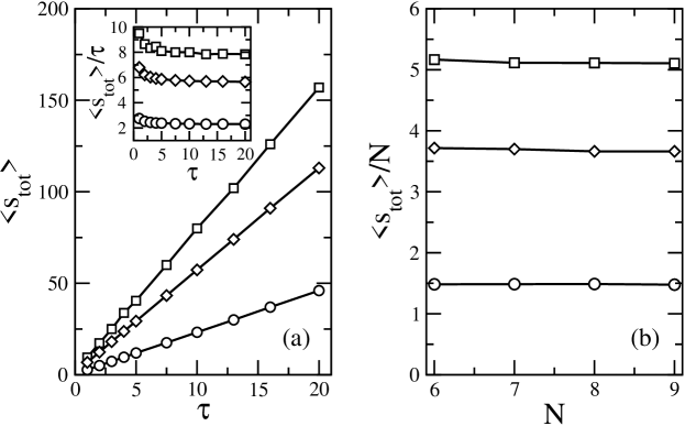
Figure 2: Mean entropy production in the steady state as a function of the total measurement time $\tau$ (left) and system size $N$ (right) for models $M_{2}^{\prime}$ (circles), $M_{2}$ (squares) and $M_{3}$ (diamonds). The parameters are $D=1$, $h=0.5$, $\lambda=1$ and $\varepsilon=0.01$, with (a) $N=8$ and (b) $\tau=5$ for the right panel. Both the average entropy production per unit time, see inset in (a), as well as the average entropy production per site reach rapidly a constant value.

IV.2 The long time limit

As discussed in Section III the long-time properties of the entropy production are encoded in the eigenvalue $\nu(\mu)$ of the linear operator $L_{\mu}$. After having determined $\nu(\mu)$ we can use that quantity in order to discuss the mean entropy production rate, see Eq. (11), as well as the large deviation function for the entropy production, see Eq. (12).

IV.2.1 The mean entropy production rate

In Fig. 3 we show examples of changes of the mean entropy production rate $\left<\dot{s}_{m}\right>$ for various systems when varying one of the system parameters. Fig. 3a illustrates some of our results for the reaction-diffusion systems where the creation rate $h$ is changed and all the other system parameters are kept constant. Fig. 3b is devoted to the transport process with a varying entrance rate $\alpha$.

Interestingly, $\left<\dot{s}_{m}\right>$ encodes important information on the physical properties of the different steady states. Focusing first on the reaction-diffusion systems, we see that for model $M_{2}^{\prime}$ the mean entropy production rate has a maximum around $h=1$ and decreases towards zero for larger values of the creation rate. In stark contrast to this $\left<\dot{s}_{m}\right>$ increases monotonously for the other two models $M_{2}$ and $M_{3}$. In order to understand this difference in behavior, we refer the reader to the reaction schemes listed in Table 1. Noting that for very large values of $h$ there is an increased probability for a free site to be surrounded by occupied neighboring sites, it follows that the creation process $0\to A$ is then effectively identical to the process $A\to 2A$. This is, however, exactly the reversed reaction to the annihilation process of model $M_{2}^{\prime}$, such that this system approaches an equilibrium system for very large values of $h$. Consequently, the mean entropy production rate vanishes in that limit as no entropy production takes place in equilibrium. This is different for models $M_{2}$ and $M_{3}$, as here the reaction $A\to 2A$ is not the direct back-reaction of the creation process, and the systems remain out of equilibrium for any value of $h$.

Similar conclusions are also drawn when varying other system parameters. For example, when $\varepsilon\longrightarrow 1$, all reactions become symmetric, and the system approaches equilibrium. Concomitantly, the mean entropy production rate approaches zero in that limit.

It is worth noting that the behavior of the mean entropy production rate is similar to that of a quantity derived from the stationary probability currents Zia06 ; Zia07 ; Pla10 that has been proposed as a possible measure for the non-equilibrium character of a system. For example, both quantities show a non-monotonous change for model $M_{2}^{\prime}$ when increasing $h$, whereas their increase is monotonous for models $M_{2}$ and $M_{3}$ (see Fig. 2 in Dor09 ).

 

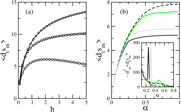
Figure 3: (Color online) Mean entropy production rate $\left<\dot{s}_{m}\right>$ for (a) reaction-diffusion systems $M_{2}^{\prime}$ (circles), $M_{2}$ (squares) and $M_{3}$ (diamonds) as a function of the creation rate $h$ (values of other parameters: $N=8$, $D=0.5$, $\varepsilon=0.01$, with $\lambda=5$ for model $M_{2}^{\prime}$ and $\lambda=0.1$ for models $M_{2}$ and $M_{3}$), and (b) the PASEP as a function of the entrance rate $\alpha$ (full black line: exit rate $\beta=0.25$; gray line: $\beta=0.30$; dashed black line: $\beta=0.5$; green (dark gray) line: $\beta=0.75$) with $N=8$, $p=0.95$ and $\varepsilon=0.01$. Inset in (b): the negative of the second derivative of $\left<\dot{s}_{m}\right>$ with respect to $\alpha$ reveals the existence of a kink in the mean entropy production rate for $\alpha=\beta\lessapprox 0.46$. For larger values of $\beta$ only a small peak remains, the position of which is $\alpha\approx 0.47$, independent of the value of $\beta$.

Non-trivial information is also contained in the mean entropy production rate of the transport process. As an example we show in Fig. 3b $\left<\dot{s}_{m}\right>$ as a function of the entrance rate $\alpha$ for a strongly asymmetric case with $p=0.95$. The striking feature in this figure is the appearance of kinks in the curves obtained for smaller exit rates, as for example $\beta=0.25$ or $\beta=0.30$. These kinks, which are located at $\alpha=\beta$, yield a sharp peak in the negative of the second derivative of $\left<\dot{s}_{m}\right>$ with respect to $\alpha$, see inset of Fig. 3b. We checked that these kinks show up for all $\beta\lessapprox 0.46$ at the value $\alpha=\beta$. For larger values of $\beta$ the kink vanishes and only a small peak remains in the second derivative (the peak still exists for $\beta=0.75$ but is not visible on the scale of the inset in Fig. 3b). Interestingly, in this regime the position of the peak is independent of the value of $\beta$ and is given by $\alpha\approx 0.47$.

In order to understand this result we need to remind the reader of the phase diagram of the PASEP San94 . For our choice of entrance and exit rates at the boundaries of the system the phase diagram of the PASEP is very similar to that of the TASEP and contains a low density phase, a high density phase and a maximum current phase. The phase boundary between the low and the high density phases, which is discontinuous and characterized by the coexistence of these two phases, is given by $\alpha=\beta$, $\alpha<r_{c}$, where $r_{c}$ depends on the specific values of the different rates. In addition, one has that the boundary between the low density (high density) phase and the maximum current phase is given by $\alpha=r_{c}$ and $\beta>r_{c}$ ($\alpha>r_{c}$ and $\beta=r_{c}$). Insertion of the values of the rates used in Fig. 3b into the exact expressions for the phase boundaries San94 yields the value $r_{c}=0.45\overline{45}$. Comparing this with the position of the kink in the mean entropy production rate for $\beta\lessapprox 0.46$, we see that the kink coincides with the discontinuous transition separating the low from the high density phase. In addition, for $\beta>r_{c}$ the extremum of the second derivative of $\left<\dot{s}_{m}\right>$ close to $\alpha\approx r_{c}$ indicates the transition separating the low density phase from the maximum current phase.

IV.2.2 Large deviation function for the entropy production

In order to compute the large deviation function for the entropy production, we proceed as discussed in Section III and determine the lowest eigenvalue $\nu(\mu)$ of the linear operator $L_{\mu}$, see Eq. (III). The large deviation function is then obtained through the Legendre transform (12).

Typical results obtained for our systems are shown in Fig. 4 where the left column is devoted to the reaction-diffusion systems and the right one to the PASEP. As expected, the eigenvalue $\nu(\mu)$ fulfills the relation (14) that follows directly from the fluctuation theorem, see Fig. 4a and Fig. 4d. By construction, the large deviation function $\chi(\sigma)$ is zero at $\sigma=1$. In addition, plots of $\chi(\sigma)$, see Fig. 4b and Fig. 4e, reveal for all studied situations a kink at zero entropy production $\sigma=0$. This kink is best revealed when studying the derivatives of $\chi$ with respect to $\sigma$, as shown in Fig. 4c and Fig. 4e, yielding a step at $\sigma=0$ in the first derivative and a maximum at $\sigma=0$ in the second derivative.

 

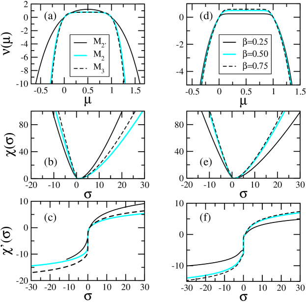
Figure 4: (Color online) (a,d) The lowest eigenvalue $\nu(\mu)$ of the linear operator $L_{\mu}$, (b,e) the large deviation function for the energy production $\chi(\sigma)$, and (c,f) the derivative of the large deviation function for (a,b,c) the reaction-diffusion models shown in Fig. 3a, with $N=8$, $h=2$, $D=0.5$, $\varepsilon=0.01$, $\lambda=5$ for model $M_{2}^{\prime}$ and $\lambda=0.1$ for models $M_{2}$ and $M_{3}$, and (d,e,f) the transport processes discussed in Fig. 3b, with $N=8$, $\alpha=0.6$, $p=0.95$ and $\varepsilon=0.01$. In all studied cases, the large deviation function exhibits a kink at zero entropy production, $\sigma=0$

As stressed in the Introduction, a kink has also been observed recently in a study of the steady-state entropy production for a single particle driven along a periodic potential Meh08 . The fact that a similar behavior is observed in our interacting many-body systems suggests that this feature is a universal one.

Before discussing the origin of the kink further, let us briefly pause and discuss how the large deviation function and its derivative depend on the parameters of the system. As an example, we show in Fig. 5 $\chi$ and $\chi^{\prime}$ for the reaction-diffusion model $M_{3}$ for various values of the creation field $h$. In our discussion of the mean entropy production rate we pointed out that for this system $\left<\dot{s}_{m}\right>$ increases when $h$ increases, resulting in an enhanced non-equilibrium character when taking $\left<\dot{s}_{m}\right>$ as a measure. Interestingly, the kink in the large deviation function also gets more pronounced when $h$ increases, as witnessed by a larger amplitude of the step in the derivative $\chi^{\prime}$. This is the generally observed behavior for all our systems: when the system parameters are varied in such a way that the mean entropy production rate increases (decreases), then the step height at $\sigma=0$ of the derivative of the large deviation function also increases (decreases).

 

Figure 5: (Color online) (a) The large deviation function of the entropy production and (b) its derivative for model $M_{3}$ and different values of the creation rate $h$. The parameters used for this figure are $N=8$, $D=0.5$, $\lambda=0.1$, and $\varepsilon=0.01$. For $\sigma=0$ a kink shows up in the large deviation function which is best illustrated by the rapid change in its derivative with respect to $\sigma$.

In fact, the kink at $\sigma=0$ in the large deviation function for the entropy production is a generic feature and immediately follows from the fluctuation theorem Eva93 ; Gal95 ; Kur98 ; Leb99 . To see this, we remind the reader that the fluctuation theorem shows up on the level of the large deviation function through the symmetry relation (13). Taking the derivative of that relation with respect to $\sigma$ yields the following relations between the derivatives at both sides of $\sigma=0$:

$$\left.\frac{d\chi}{d\sigma}\right|_{\sigma=\sigma_{0}}+\left.\frac{d\chi}{d\sigma}\right|_{\sigma=-\sigma_{0}} = -\left<\dot{s}_{m}\right>$$ (15)

$$\left.\frac{d\chi}{d\sigma}\right|_{\sigma=\sigma_{0}}-\left.\frac{d\chi}{d\sigma}\right|_{\sigma=-\sigma_{0}} = 2\left.\frac{d\chi}{d\sigma}\right|_{\sigma=\sigma_{0}}+\left<\dot{s}_{m}\right>$$ (16)

valid for any value of the entropy production $\sigma_{0}$. In Fig. 6 we illustrate for model $M_{3}$ the relation (13) for the large deviation function as well as the relations (15) and (16) for its derivative.

 

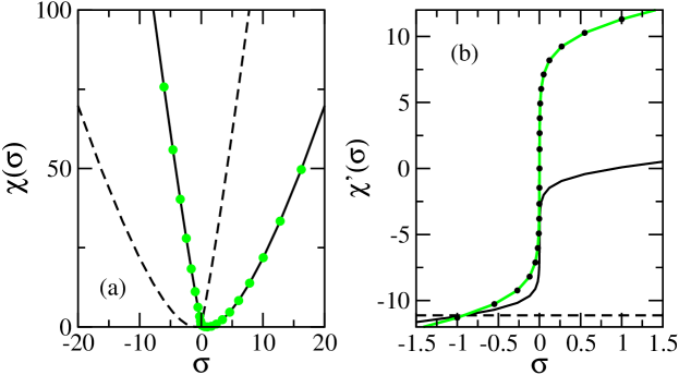
Figure 6: (Color online) (a) Illustration of the symmetry relation (13) for model $M_{3}$ with $N=8$, $D=0.5$, $\varepsilon=0.01$, $h=2$, and $\lambda=0.1$. The full line is $\chi(\sigma)$, the dashed line is $\chi(-\sigma)$, whereas the green (gray) circles follow from $\chi(-\sigma)-\sigma\left<\dot{s}_{m}\right>$. For the chosen set of parameters we have that $\left<\dot{s}_{m}\right>=11.1228$. (b) Illustration of relations (15) and (16) of the derivative $\chi^{\prime}$ of the large deviation function. Full black line: $\chi^{\prime}(\sigma)$; dashed black line: $\chi^{\prime}(\sigma)+\chi^{\prime}(-\sigma)$; green (gray) line: $\chi^{\prime}(\sigma)-\chi^{\prime}(-\sigma)$; black circles: $2\chi^{\prime}(\sigma)+\left<\dot{s}_{m}\right>$.

The relations (15) and (16) completely characterize the kink. In fact, one really should describe the observed feature as kink-like, as the derivative of $\chi$ is still continuous at $\sigma=0$ even though its value changes rather dramatically when the entropy production approaches zero. Eqs. (15) and (16) make obvious the connection between the kink and the mean entropy production rate. It is the value of $\left<\dot{s}_{m}\right>$ that characterizes this intriguing behavior of the large deviation function of the entropy production. A larger value of $\left<\dot{s}_{m}\right>$ yields a more pronounced feature and a sharper and higher peak in the second derivative of the large deviation function.

One might object that in some known cases the distribution of the entropy production has a nearly Gaussian form and that for these cases a kink-like behavior is not observed. An example can be found in Ref. Meh08 (see their Figures 1 and 3), where the large deviation function for a particle driven along a periodic potential is nicely fitted to a parabola

$$\chi(\sigma)=\left(\langle\dot{s}_{m}\rangle/4\right)\left(\sigma-1\right)^{2}$$ (17)

for small forces. In a similar way, the largest eigenvalue seems to be well described by

$$\nu(\mu)=\langle\dot{s}_{m}\rangle\mu(1-\mu)~{}.$$ (18)

These results seem to indicate that close to equilibrium systems with a nearly Gaussian entropy production can fulfill the fluctuation theorem without exhibiting a kink-like feature in the large deviation function.

 

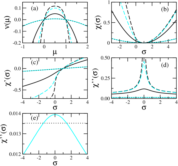
Figure 7: (Color online) Discussion of the transport process with $\alpha=\beta=0.5$ and $p=0.5$. The different curves correspond to various values of $\varepsilon$: 0.001 (dashed black line), 0.01 (dashed gray [magenta] line), 0.1 (full black line), and 0.5 (full gray [magenta] line). (a) Lowest eigenvalue $\nu(\mu)$ of the linear operator $L_{\mu}$, (b) large deviation function for the entropy function $\chi(\sigma)$, (c) first derivative of the large deviation function, (d) second derivative of the large deviation function, and (e) second derivative of the large deviation function for $\varepsilon=0.5$. The dotted lines result from fitting the data for $\varepsilon=0.5$ to the quadratic forms (17) and (18). Systematic deviations between the data and the fit are readily observed in $\chi^{\prime\prime}(\sigma)$.

Our systems allow us to address this point in a systematic way. In fact, we always find for systems that are close to equilibrium (as characterized by a small value of the mean entropy production rate) that the entropy production approaches a nearly Gaussian form and that the kink seems to vanish. This is illustrated in Fig. 7 for the transport process with $\alpha=\beta=p=0.5$ and various values of $\varepsilon$. In this case the system approaches equilibrium when $\varepsilon$ increases, yielding an equilibrium system for $\varepsilon=1$. As we see from Fig. 7a and 7b, the kink-like feature in the large deviation function gets less and less pronounced when increasing $\varepsilon$ and seems to have vanished completely for $\varepsilon=0.5$. Indeed, in that case one can fit the largest eigenvalue and the large deviation function to the quadratic forms (18) and (17), thereby obtaining an excellent agreement. However, a closer look at the second derivative, see Fig. 7d and 7e, reveals that qualitatively the case $\varepsilon=0.5$ does not differ from the other cases: the second derivative exhibits a maximum at $\sigma=0$ which is the signature of the kink-like feature. Admittedly, this maximum is rather shallow for a system close to equilibrium, but it persists as long as the mean entropy production rate does not vanish. Obviously, it is not good enough to simply fit the data to the quadratic forms (17) and (18) and to conclude from an optically good fit that the kink-like behavior is absent. The kink-like feature might no longer be easily detectable by simple inspection of $\chi$ in systems where the entropy production approaches a nearly Gaussian form, but it still reveals itself in a maximum in $\chi^{\prime\prime}(\sigma)$.

From our study, as well as from the observation of kink-like features in other systems fulfilling the fluctuation theorem, we can therefore conclude that this behavior is generic for non-equilibrium systems.

V Conclusion

Our study of interacting many-body systems has yielded two main results regarding the entropy production in the steady states of non-equilibrium systems.

On the one hand, we showed that the kink observed in the entropy production large deviation function at zero entropy production is generic and directly follows from the fluctuation theorem. The well known relation for the large deviation function (13) implies certain relations between the derivatives on both sides of $\sigma=0$, see Eq. (15) and (16). It follows that the kink is characterized by the value of the mean entropy production rate in the steady state.

On the other hand, our results indicate that the mean entropy production rate is a good measure for quantifying the non-equilibrium character of a system (or, equivalently, the degree of violation of detailed balance). Not only does it characterize the kink-like structure in the large deviation function, it also directly reveals whether a system gets closer to be an equilibrium system when changing some system parameters, as illustrated in Fig. 3a. In addition, the mean entropy production rate also reveals the presence of dynamic phase transitions, as seen in our study of the PASEP, see Fig. 3b.

Recently Zia06 ; Zia07 ; Pla10 it was proposed that the non-equilibrium character of a system can be captured quantitatively by some global observables derived from the probability currents. Probability currents and entropy production are of course intimately related. They are unique to a non-equilibrium system and are absent in equilibrium systems. They also show a remarkably similar dependence on system parameters. As an example, the reader should compare our Fig. 3a with Fig. 2 in Dor09 where these quantities are computed for the one-dimensional reaction-diffusion systems discussed in this manuscript. To our knowledge, however, it has not yet been studied whether the observable derived from the stationary probability currents allows to probe the system for the presence of a phase transition. A more systematic comparison of the behavior of that quantity with that of the mean entropy production rate seems to be needed in order to further elucidate the commonalities and differences between these two quantities.

As a final remark we note that in the past quite some effort has been devoted to the computation and understanding of the current large deviation function in driven systems. In our study we focused on the large deviation function of the entropy production and characterized its properties both for systems with (PASEP) and without (reaction-diffusion systems) particle currents. The exact relation between these two large deviation functions in driven systems remains to be better understood.

- (1) R. S. Ellis, Entropy, Large Deviations, and Statistical Mechanics (Berlin, Springer, 1985).
- (2) A. Dembo and O. Zeitouni, Large Deviation Techniques and Applications (Berlin, Springer, 1998).
- (3) H. Touchette, Phys. Rep. 478, 1 (2009).
- (4) L. Bertini, A. De Sole, D. Gabrielli, G. Jona-Lasinio, and C. Landim, J. Stat. Mech. P07014 (2007).
- (5) B. Derrida, J. Stat. Mech. P07023 (2007).
- (6) J. Mehl, T. Speck, and U. Seifert, Phys. Rev. E 78, 011123 (2008).
- (7) J. L. Lebowitz and H. Spohn, J. Stat. Phys. 95, 333 (1999).
- (8) P. Visco, J. Stat. Mech. P06006 (2006).
- (9) K. Turitsyn, M. Chertkov, V. Y. Chernyak, and A. Puliafito, Phys. Rev. Lett. 98, 180603 (2007).
- (10) B. Cleuren, C. Van den Broeck, and R. Kawai, C. R. Physique 8, 567 (2007).
- (11) D. Lacoste, A. W. C. Lau, and K. Mallick, Phys. Rev. E 78, 011915 (2008).
- (12) N. Kumar, S. Ramaswamy, and A. K. Sood, arXiv:1009.5925.
- (13) In most of these papers the authors did not discuss the kink explicitly. However, in all cases the existence of the kink can either be derived from the exact expressions given for the large deviation functions or it can be inferred from the numerical data shown in various figures.
- (14) R. A. Blythe and M. R. Evans, J. Phys. A: Math. Theor. 40, R333 (2007).
- (15) B. Derrida and J. L. Lebowitz, Phys. Rev. Lett. 80, 209 (1998).
- (16) B. Derrida and C. Appert, J. Stat. Phys. 94, 1 (1999).
- (17) D. Kim, Phys. Rev. E 52, 3512 (1995).
- (18) V. Lecomte, U. C. Täuber, and F. van Wijland, J. Phys. A: Math. Theor. 40, 1447 (2007).
- (19) T. Bodineau and M. Lagouge, J. Stat. Phys. 139, 201 (2010).
- (20) D. Simon, arXiv:1011.3590.
- (21) M. Henkel, H. Hinrichsen, and S. Lübeck, Non-Equilibrium Phase Transitions: Volume 1: Absorbing Phase Transitions (Springer/Dordrecht and Canopus/Bristol, 2008).
- (22) G. Ódor, Universality in Nonequilibrium Lattice Systems: Theoretical Foundations (World Scientific/Singapore, 2008).
- (23) B. Derrida, Phys. Rep. 301, 65 (1998).
- (24) G. M. Schütz, in Phase Transitions and Critical Phenomena, edited by C. Domb and J. Lebowitz (Academic Press, London, 2001), Vol. 19.
- (25) O. Golinelli and K. Mallick, J. Phys. A: Math. Gen. 39, 12679 (2006).
- (26) S. Dorosz and M. Pleimling, Phys. Rev. E 79, 030102(R) (2009).
- (27) S. Dorosz and M. Pleimling, Phys. Rev. E 80, 061114 (2009).
- (28) S. Dorosz and M. Pleimling, Physics Procedia 4, 107 (2010).
- (29) U. Seifert, Eur. Phys. J. B 64, 423 (2008).
- (30) D. J. Evans, E. G. D. Cohen, and G. P. Morriss, Phys. Rev. Lett. 71, 2401 (1993).
- (31) G. Gallavotti and E. G. D. Cohen, Phys. Rev. Lett. 74, 2694 (1995).
- (32) J. Kurchan, J. Phys. A 31, 3719 (1998).
- (33) U. Seifert, Phys. Rev. Lett. 95, 040602 (2005).
- (34) M. Esposito, U. Harbola, and S. Mukamel, Phys. Rev. E 76, 031132 (2007).
- (35) R. K. P. Zia and B. Schmittmann, J. Phys. A 39, L409 (2006).
- (36) R. K. P. Zia and B. Schmittmann, J. Stat. Mech. P07012 (2007).
- (37) T. Platini, arXiv:1007.0165.
- (38) S. Sandow, Phys. Rev. E 50, 2660 (1994).