Dynamic Coalitional TU Games: Distributed Bargaining among Players’ Neighbors

Abstract

We consider a sequence of transferable utility (TU) games where, at each time, the characteristic function is a random vector with realizations restricted to some set of values. The game differs from other ones in the literature on dynamic, stochastic or interval valued TU games as it combines dynamics of the game with an allocation protocol for the players that dynamically interact with each other. The protocol is an iterative and decentralized algorithm that offers a paradigmatic mathematical description of negotiation and bargaining processes. The first part of the paper contributes to the definition of a robust (coalitional) TU game and the development of a distributed bargaining protocol. We prove the convergence with probability 1 of the bargaining process to a random allocation that lies in the core of the robust game under some mild conditions on the underlying communication graphs. The second part of the paper addresses the more general case where the robust game may have empty core. In this case, with the dynamic game we associate a dynamic average game by averaging over time the sequence of characteristic functions. Then, we consider an accordingly modified bargaining protocol. Assuming that the sequence of characteristic functions is ergodic and the core of the average game has a nonempty relative interior, we show that the modified bargaining protocol converges with probability 1 to a random allocation that lies in the core of the average game.

1 Introduction

Coalitional games with transferable utilities (TU) have been introduced by von Neumann and Morgenstern [27]. A coalitional TU game constitutes of a set of players, who can form coalitions, and a characteristic function that provides a value for each coalition. The value of a coalition can be thought of as a monetary value that can be divided among the members of the coalition according to some appropriate fairness allocation rule.

Coalitional TU games have been used to model cooperation in supply chain or inventory management applications [6, 10], as well as in network flow applications to coordinate flows of goods, materials, or resources between different production/distribution sites [2]. Recently, coalitional games have also sparked much interest in communication networks. We refer an interested reader to tutorial [23] for an in-depth discussion on potential applications in this field.

In this paper, we consider a sequence of coalitional TU games for a finite set of players. We assume that the game is played repeatedly over time thus generating a sequence of time varying characteristic functions. We refer to such a repeated game as dynamic coalitional TU game. In addition, we assume that a player need not necessarily observe the allocations of all the other players, but he can only observe the allocations of his neighbors, where the neighbors may change in time.

In this setting, we consider robust and average TU games, and for each of these games we propose an allocation process to reach a solution of the dynamic game. More specifically, we formulate a dynamic bargaining process as a dynamically changing constrained problem. Iterations are simply bargaining steps free of any concrete reward allocation. We assume that the reward allocation occurs only once at the end of the bargaining process, when the players have agreed on how to allocate rewards among themselves. Our main objective is to explore distributed agreement on solutions in the core of the game, where the players interact only with their neighbors.

In particular, we consider bargaining protocols assuming that each player $i$ obeys rationality and efficiency by deciding on an allocation vector which satisfies the value constraints of all the coalitions that include player $i$. This set is termed bounding set of player $i$. At every iteration, a player $i$ observes the allocations of some of his neighbors. This is modeled using a directed graph with the set of players as the vertex set and a time-varying edge set composed of directed links $(i,j)$ whenever player $i$ observes the allocation vector proposed by player $j$ at time $t$. We refer to this directed graph as players’ neighbor-graph. Given a player’s neighbor-graph, each player $i$ negotiates allocations by adjusting the allocations he received from his neighbors through weight assignments. As the balanced allocation may violate his rationality constraints (it lies outside player $i$’s bounding set), the player selects a new allocation by projecting the balanced allocation on his bounding set. We propose such bargaining protocols for solving both the robust and the average TU game. For each of these games, we use some mild assumptions on the connectivity of the players’ neighbor-graph and the weights that the players use when balancing their own allocations with the neighbors’ allocations. Assuming that the core of the robust game is nonempty, we show that our bargaining protocol converges with probability 1 to a common (random) allocation in the core. In the case when the core of the robust game is empty, we consider an average game that can provide a meaningful solution under some conditions on the sequence of the characteristic functions. Specifically, in this case, we consider a dynamic average game by averaging over time the sequence of characteristic functions. We then modify accordingly the bounding set and the associated bargaining process by using the dynamic average game. This means that the value constraints are defined by using the time-averaged sequence rather than the sequence of random characteristic functions. Under the assumptions that the time-averaged sequence is ergodic and that the core of the average game has a nonempty relative interior, we show that the players’ allocations generated by our bargaining protocol converge with probability 1 to a common (random) allocation in the core of the average game.

The main contributions of this paper are in the two-fold dynamic aspect of the games, and in the development and the analysis of distributed bargaining process among the players. The novelty in the dynamic aspect is in the consideration of games with time-varying characteristic functions and the use of time-varying local players interactions.

The work in this paper is related to stochastic cooperative games [9, 24, 25]. However, we deviate from this stochastic framework in a number of aspects among which are the existence of a local players interactions captured by players’ neighbor-graph and the presence of multiple iterations in the bargaining process, and the consideration of robust game. Bringing dynamical aspects into the framework of coalitional TU games is an element in common with papers [8, 11]. However, unlike [8, 11], the values of the coalitions in this paper are realized exogenously and no relation is assumed between consecutive samples. Dynamic robust TU games have been considered in [3] and [4] but for a continuous time setting in the former work and for a centralized allocation process in the latter one. Convergence of allocation processes is a main topic in [5, 13]. There, rewards are allocated by a game designer repeatedly in a centralized manner and based on the current excess rewards of the coalitions (accumulated reward up to current time minus the value of the coalition). Our approach, however, differs from that of [5, 13] as we resort to a decentralized scheme where the allocation process is the result of a bargaining process among the players with local interactions. Convergence of bargaining processes has also been explored under dynamic coalition formation [1] for a different dynamic model, where players decide both on which coalition to address and what payoff to announce. Coalitions form when announced payoffs are all met for all players in the coalition. Our bargaining procedure is different as it produces an agreement resulting in the formation of grand coalition, which is stable with respect to any sub-coalitions.

The work in this paper is also related to the literature on agreement among multiple agents, where an underlying communication graph for the agents and balancing weights have been used with some variations [26, 15] to reach an agreement on common decision variable, as well as in [16, 17, 20, 19] for distributed multi-agent optimization.

This paper is organized as follows. In Section 2, we introduce the dynamic TU game, the robust game and the bargaining protocol for this game. We then motivate the game and give some preliminary results. In Section 3, we prove the convergence of the bargaining protocol to a point in the core of the robust game with probability 1. In Section 4, we introduce the dynamic average game and the modified bargaining protocol. We also prove the convergence of this protocol to an allocation in the core of the average game with probability 1. In Section 5, we report some numerical simulations to illustrate our theoretical study, and we conclude in Section 6.

Notation. We view vectors as columns. For a vector $x$, we use $x_{i}$ or $[x]_{i}$ to denote its $i$th coordinate component. For two vectors $x$ and $y$, we use $x<y$ ($x\leq y$) to denote $x_{i}<y_{i}$ ($x_{i}\leq y_{i}$) for all coordinate indices $i$. We let $x^{\prime}$ denote the transpose of a vector $x$, and $\|x\|$ denote its Euclidean norm. An $n\times n$ matrix $A$ is row-stochastic if the matrix has nonnegative entries $a_{ij}$ and $\sum_{j=1}^{n}a_{ij}=1$ for all $i=1,\ldots,n$. For a matrix $A$, we use $a_{ij}$ or $[A]_{ij}$ to denote its $ij$th entry. A matrix $A$ is doubly stochastic if both $A$ and its transpose $A^{\prime}$ are row-stochastic. Given two sets $U$ and $S$, we write $U\subset S$ to denote that $U$ is a proper subset of $S$. We use $|S|$ for the cardinality of a given finite set $S$.

We write $P_{X}[x]$ to denote the projection of a vector $x$ on a set $X$, and we write ${\rm dist}(x,X)$ for the distance from $x$ to $X$, i.e., $P_{X}[x]=\arg\min_{y\in X}\|x-y\|$ and ${\rm dist}(x,X)=\|x-P_{X}[x]\|$, respectively. Given a set $X$ and a scalar $\lambda\in\mathbb{R}$, the set $\lambda X$ is defined by $\lambda X\triangleq\{\lambda x\mid x\in X\}$. Given two sets $X,Y\subseteq\mathbb{R}^{n}$, the set sum $X+Y$ is defined by $X+Y\triangleq\{x+y\mid x\in X,\ y\in Y\}$. Given a set $N$ of players and a function $\eta:S\mapsto\mathbb{R}$ defined for each nonempty coalition $S\subseteq N$, we write $<N,\eta>$ to denote the transferable utility (TU) game with the players’ set $N$ and the characteristic function $\eta$. We let $\eta_{S}$ be the value $\eta(S)$ of the characteristic function $\eta$ associated with a nonempty coalition $S\subseteq N$. Given a TU game $<N,\eta>$, we use $C(\eta)$ to denote the core of the game, $C(\eta)=\left\{x\in\mathbb{R}^{|N|}\,\Big{|}\,\sum_{i\in N}x_{i}=\eta_{N},\ \sum_{i\in S}x_{i}\geq\eta_{S}\hbox{ for all nonempty }S\subset N\right\}.$

2 Dynamic TU Game and Robust Game

In this section, we discuss the main components of a dynamic TU game and a robust game. We state some basic assumptions on these games and introduce a bargaining process conducted by the players to reach an agreement on their allocations. We also provide some examples of the TU games motivating our development and establish some basic results that we use later on in the convergence analysis of the bargaining process.

2.1 Problem Formulation and Bargaining Process

Consider a set of players $N=\{1,\ldots,n\}$ and the set of all (nonempty) coalitions $S\subseteq N$ arising among these players. Let $m=2^{n}-1$ be the number of possible coalitions. We assume that the time is discrete and use $t=0,1,2,\ldots$ to index the time slots.

We consider a dynamic TU game, denoted $<N,\{v(t)\}>$, where $\{v(t)\}$ is a sequence of characteristic functions. Thus, in the dynamic TU game $<N,\{v(t)\}>$, the players are involved in a sequence of instantaneous TU games whereby, at each time $t$, the instantaneous TU game is $<N,v(t)>$ with $v(t)\in\mathbb{R}^{m}$ for all $t\geq 0$. Further, we let $v_{S}(t)$ denote the value assigned to a nonempty coalition $S\subseteq N$ in the instantaneous game $<N,v(t)>$. In what follows, we deal with dynamic TU games where each characteristic function $v(t)$ is a random vector with realizations restricted to some set of values. We will consider the robust TU game in this section and Section 3, while in Section 4 we deal with the average TU game.

In our development of robust TU game, we impose restrictions on each realization of $v(t)$ for every $t\geq 0$. Specifically, we assume that the grand coalition value $v_{N}(t)$ is deterministic for every $t\geq 0$, while the values $v_{S}(t)$ of the other coalitions $S\subset N$ have a common upper bound. These conditions are formally stated in the following assumption.

Assumption 1

There exists $v^{\max}\in\mathbb{R}^{m}$ such that for all $t\geq 0$,

$$v_{N}(t)=v_{N}^{\max},$$

$$v_{S}(t)\leq v_{S}^{\max}\qquad\hbox{for all nonempty coalitions }S\subset N.$$

We refer to the game $<N,v^{\max}>$ as robust game. In the first part of this paper, we rely on the assumption that the robust game has a nonempty core.

Assumption 2

The core $C(v^{\max})$ of the robust game is not empty.

An immediate consequence of Assumptions 1 and 2 is that the core $C(v(t))$ of the instantaneous game is always not empty. This follows from the fact that $C(v^{\rm max})\subseteq C(\eta)$ for any $\eta$ satisfying $\eta_{N}=v^{\rm max}_{N}$ and $\eta_{S}\leq v^{\rm max}_{S}$ for $S\subset N$, and the assumption that the core $C(v^{\rm max})$ is not empty.

Throughout the paper, we assume that each player $i$ is rational and efficient. This translates to each player $i\in N$ choosing his allocation vector within the set of allocations satisfying value constraints of all the coalitions that include player $i$. This set is referred to as the bounding set of player $i$ and, for a generic game $<N,\eta>$, it is given by

$$X_{i}(\eta)=\left\{x\in\mathbb{R}^{n}\mid\sum_{j\in N}x_{j}=\eta_{N},\ \sum_{j\in S}x_{j}\geq\eta_{S}\ \mbox{for all $S\subset N$ s.t.~{}}i\in S\right\}.$$

Note that each $X_{i}(\eta)$ is polyhedral.

In what follows, we find it suitable to represent the bounding sets and the core in alternative equivalent forms. For each nonempty coalition $S\subseteq N$, let $e_{S}\in\mathbb{R}^{n}$ be the incidence vector for the coalition $S$, i.e., the vector with the coordinates given by

$$[e_{S}]_{i}=\left\{\begin{array}[]{ll}1&\hbox{if $i\in S$,}\cr 0&\hbox{else}.\end{array}\right.$$

Then, the bounding sets and the core can be represented as follows:

$$X_{i}(\eta)=\{x\in\mathbb{R}^{n}\mid e^{\prime}_{N}x=\eta_{N},\ e_{S}^{\prime}x\geq\eta_{S}\ \hbox{for all $S\subset N$ with $i\in S$}\},$$ (1)

$$C(\eta)=\{x\in\mathbb{R}^{n}\mid e^{\prime}_{N}x=\eta_{N},\ e_{S}^{\prime}x\geq\eta_{S}\ \hbox{for all nonempty $S\subset N$}\}.$$ (2)

Furthermore, observe that the core $C(\eta)$ of the game coincides with the intersection of the bounding sets $X_{i}(\eta)$ of all players $i\in N=\{1,\ldots,n\}$, i.e.,

$$C(\eta)=\cap_{i=1}^{n}X_{i}(\eta).$$ (3)

We now discuss the bargaining protocol where repeatedly over time each player $i\in N$ submits an allocation vector that the player would agree on. The allocation vector proposed by player $i$ at time $t$ is denoted by $x^{i}(t)\in\mathbb{R}^{n}$, where the $j$th component $x_{j}^{i}(t)$ represents the amount that player $i$ would assign to player $j$. To simplify the notation in the dynamic game $<N,\{v(t)\}>$, we let $X_{i}(t)$ denote the bounding set of player $i$ for the instantaneous game $<N,v(t)>$, i.e., for all $i\in N$ and $t\geq 0$,

$$X_{i}(t)=\left\{x\in\mathbb{R}^{n}\mid\sum_{j\in N}x_{j}=v_{N}(t),\ \sum_{j\in S}x_{j}\geq v_{S}(t)\mbox{ for all $S\subset N$ s.t.~{}}i\in S\right\}.$$ (4)

We assume that each player may observe the allocations of a subset of the other players at any time, which are termed as the neighbors of the player. The players and their neighbors at time $t$ can be represented by a directed graph $\mathcal{G}(t)=(N,\mathcal{E}(t))$, with the vertex set $N$ and the set $\mathcal{E}(t)$ of directed links. A link $(i,j)\in\mathcal{E}(t)$ exists if player $j$ is a neighbor of player $i$ at time $t$. We always assume that $(i,i)\in\mathcal{E}(t)$ for all $t$, which is natural since every player $i$ can always access its own allocation vector. We refer to graph $\mathcal{G}(t)$ as a neighbor-graph at time $t$. In the graph $\mathcal{G}(t)$, a player $j$ is a neighbor of player $i$ (i.e., $(i,j)\in\mathcal{E}(t)$) only if player $i$ can observe the allocation vector of player $j$ at time $t$. Figure 1 illustrates how the players’ neighbor-graph may look at two time instances.

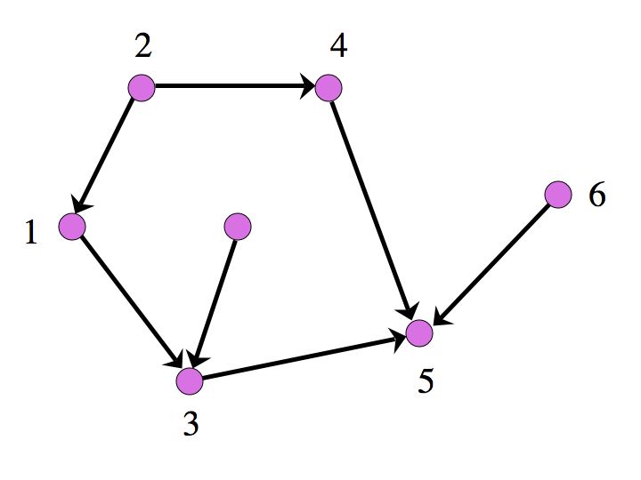
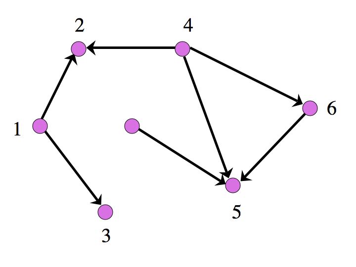
Figure 1: Players’ neighbor graphs for 6 players and two different time instances.

Given the players’ neighbor-graph $\mathcal{G}(t)$, each player $i$ negotiates allocations by averaging his allocation and the allocations he received from his neighbors. More precisely, at time $t$, the bargaining process for each player $i$ involves the player’s individual bounding set $X_{i}(t)$, its own allocation $x^{i}(t)$ and the observed allocations $x^{j}(t)$ of some of his neighbors $j$. Formally, we let $\mathcal{N}_{i}(t)$ be the set of neighbors of player $i$ at time $t$ (including himself), i.e.,

$$\mathcal{N}_{i}(t)=\{j\in N\mid(i,j)\in\mathcal{E}(t)\}.$$

With this notation, the bargaining process is given by:

$$x^{i}(t+1)=P_{X_{i}(t)}\left[\sum_{j\in\mathcal{N}_{i}(t)}a_{ij}(t)x^{j}(t)\right]\qquad\hbox{for all $i\in N$ and $t\geq 0$},$$ (5)

where $a_{ij}(t)\geq 0$ is a scalar weight that player $i$ assigns to the proposed allocation $x^{j}(t)$ of player $j$ and $P_{X_{i}(t)}[\cdot]$ is the projection onto the player $i$ bounding set $X_{i}(t)$. The initial allocations $x^{i}(0),$ $i=1,\ldots,n,$ are selected randomly and independently of $\{v(t)\}$.

The bargaining process in (5) can be written more compactly by introducing zero weights for players $j$ whose allocations are not available to player $i$ at time $t$. Specifically by defining $a_{ij}(t)=0$ for all $j\not\in\mathcal{N}_{i}(t)$ and all $t\geq 0$, we have the following equivalent representation of the bargaining process:

$$x^{i}(t+1)=P_{X_{i}(t)}\left[\sum_{j=1}^{n}a_{ij}(t)x^{j}(t)\right]\qquad\hbox{for all $i\in N$ and $t\geq 0$}.$$ (6)

Here, $a_{ij}(t)=0$ for all $j\not\in\mathcal{N}_{i}(t)$ while $a_{ij}(t)\geq 0$ for $j\in\mathcal{N}_{i}(t)$.

We now discuss the specific assumptions on the weights $a_{ij}(t)$ and the players’ neighbor-graph that we will rely on. We let $A(t)$ be the weight matrix with entries $a_{ij}(t)$. We will use the following assumption for the weight matrices.

Assumption 3

Each matrix $A(t)$ is doubly stochastic with positive diagonal. Furthermore, there exists a scalar $\alpha>0$ such that

$$a_{ij}(t)\geq\alpha\qquad\hbox{whenever}\quad a_{ij}(t)>0.$$

In view of the construction of matrices $A(t)$, we see that $a_{ij}(t)\geq\alpha$ for $j=i$ and perhaps for some players $j$ that are neighbors of player $i$. The requirement that the positive weights are uniformly bounded away from zero is imposed to ensure that the information from each player diffuses to his neighbors in the network persistently in time. The requirement on the doubly stochasticity of the weights is used to ensure that in a long run each player has equal influence on the limiting allocation vector.

It is natural to expect that the connectivity of the players’ neighbor-graphs $\mathcal{G}(t)=(N,\mathcal{E}(t))$ impacts the bargaining process. At any time, the instantaneous graph $\mathcal{G}(t)$ need not be connected. However, for the proper behavior of the bargaining process, the union of the graphs $\mathcal{G}(t)$ over a period of time is assumed to be connected, as given in the following assumption.

Assumption 4

There is an integer $Q\geq 1$ such that the graph $\left(N,\bigcup_{\tau=tQ}^{(t+1)Q-1}\mathcal{E}(\tau)\right)$ is strongly connected for every $t\geq 0$.

Assumptions 3 and 4 together guarantee that the players communicate sufficiently often to ensure that the information of each player is persistently diffused over the network in time to reach every other player. Under these assumptions, we will study the dynamic bargaining process in (6). We want to provide conditions under which the process converges to an allocation in the core of the robust game. Before this, we provide some motivating examples in the following section.

2.2 Motivations

Dynamic coalitional games capture coordination in a number of network flow applications. Network flows model flow of goods, materials, or other resources between different production/distribution sites [2]. We next provide two examples. The first one is more practically oriented and describes a supply chain application [6]. The second one is more theoretical and re-casts the problem at hand in terms of controlled flows over hyper-graphs.

2.2.1 Supply chain

A single warehouse ${\bf v}_{0}$ serves a number of retailers ${\bf v}_{i}$, $i=1,\ldots,n$, each one facing a demand $d_{i}(t)$ unknown but bounded by pre assigned values $d_{i}^{\min}\in\mathbb{R}$ and $d_{i}^{\max}\in\mathbb{R}$ at any time period $t\geq 0$. After demand $d_{i}(t)$ has been realized, retailer ${\bf v}_{i}$ must choose to either fulfill the demand or not. The retailers do not hold any private inventory and, therefore, if they wish to fulfill their demands, they must reorder goods from the central warehouse. Retailers benefit from joint reorders as they may share the total transportation cost $K$ (this cost could also be time and/or players dependent). In particular, if retailer ${\bf v}_{i}$ “plays” individually, the cost of reordering coincides with the full transportation cost $K$. Actually, when necessary a single truck will serve only him and get back to the warehouse. This is illustrated by the dashed path $({\bf v}_{0},{\bf v}_{1},{\bf v}_{0})$ in the network of Figure 2(a). The cost of not reordering is the cost of the unfulfilled demand $d_{i}(t)$.

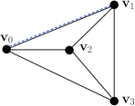
(a) Truck leaving ${\bf v}_{0}$, serving ${\bf v}_{1}$ and returning to ${\bf v}_{0}$.

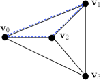
(b) Truck leaving ${\bf v}_{0}$, serving ${\bf v}_{1}$ and ${\bf v}_{2}$, and then returning to ${\bf v}_{0}$.

(c) Truck leaving ${\bf v}_{0}$, serving ${\bf v}_{1}$, ${\bf v}_{2},$ and ${\bf v}_{3}$, and then returning to ${\bf v}_{0}$.

Figure 2: Example of one warehouse ${\bf v}_{0}$ and three retailers ${\bf v}_{1}$, ${\bf v}_{2}$ and ${\bf v}_{3}$.

If two or more retailers “play” in a coalition, they agree on a joint decision (“everyone reorders” or “no one reorders”). The cost of reordering for the coalition also equals the total transportation cost that must be shared among the retailers. In this case, when necessary a single truck will serve all retailers in the coalition and get back to the warehouse. This is illustrated, with reference to coalition $\{{\bf v}_{1},{\bf v}_{2}\}$ by the dashed path $({\bf v}_{0},{\bf v}_{1},{\bf v}_{2},{\bf v}_{0})$ in Figure 2(b). A similar comment applies to the coalition $\{{\bf v}_{1},{\bf v}_{2},{\bf v}_{3}\}$ and the path $({\bf v}_{0},{\bf v}_{1},{\bf v}_{2},{\bf v}_{3},{\bf v}_{0})$ in Figure 2(c). The cost of not reordering is the sum of the unfulfilled demands of all retailers. How the players will share the cost is a part of the solution generated by the bargaining process.

The cost scheme can be captured by a game with the set $N=\{{\bf v}_{1},\ldots,{\bf v}_{n}\}$ of players where the cost of a nonempty coalition $S\subseteq N$ is given by

$$c_{S}(t)=\min\left\{K,\sum_{i\in S}d_{i}(t)\right\}.$$

Note that the bounds on the demand $d_{i}(t)$ reflect into the bounds on the cost as follows: for all nonempty $S\subseteq N$ and $t\geq 0$,

$$\min\left\{K,\sum_{i\in S}d_{i}^{\min}\right\}\leq c_{S}(t)\leq\min\left\{K,\sum_{i\in S}d_{i}^{\max}\right\}.$$ (7)

To complete the derivation of the coalitions’ values we need to compute the cost savings $v_{S}(t)$ of a coalition $S$ as the difference between the sum of the costs of the coalitions of the individual players in $S$ and the cost of the coalition itself, namely,

$$v_{S}(t)=\sum_{i\in S}c_{\{i\}}(t)-c_{S}(t).$$

Given the bound for $c_{S}(t)$ in (7), the value $v_{S}(t)$ is also bounded, as given: for any $S\subset N$ and $t\geq 0$,

$$v_{S}(t)\leq\sum_{i\in S}\min\left\{K,d_{i}^{\max}\right\}-\min\left\{K,\sum_{i\in S}d_{i}^{\min}\right\}.$$

Thus, the cost savings (value) of each coalition is bounded uniformly by a maximum value.

2.2.2 Network controlled flows

Here, we provide a more theoretical example where the bargaining process provides a way for the nodes of a hyper-graph to agree on the edge controlled flows [2]. Consider the hyper-graph $\mathcal{H}=\{V,E\}$ with the vertex set $V=\{{\bf v}_{1},\ldots,{\bf v}_{m}\}$ and the edge-set $E=\{{\bf e}_{1},\ldots,{\bf e}_{n}\}.$ The vertex set $V$ has one vertex per each coalition, while the edge-set $E$ has one edge per each player. An edge ${\bf e}_{i}$ is incident to a vertex ${\bf v}_{j}$ if the player $i$ is in the coalition associated with ${\bf v}_{j}$. For a 3-player coalitional game, the vertex-coalition correspondence is shown in Table 1. The corresponding hyper-graph is shown in Figure 3.

Figure 3: Hyper-graph $\mathcal{H}=\{V,E\}$ for a 3-player coalitional game.

	${\bf v_{1}}$	${\bf v_{2}}$	${\bf v_{3}}$	${\bf v_{4}}$	${\bf v_{5}}$	${\bf v_{6}}$	${\bf v_{7}}$
$S$	$\{1\}$	$\{2\}$	$\{3\}$	$\{1,2\}$	$\{1,3\}$	$\{2,3\}$	$\{1,2,3\}$

Table 1: Vertex-coalition correspondence for a 3-player coalitional game.

The incidence relations are described by a matrix $B_{\mathcal{H}}=[e_{S}^{\prime}]_{S\subseteq N}\in\mathbb{R}^{m\times n}$ whose rows are the characteristic vectors of all coalitions $S\subseteq N$. The flow control reformulation arises naturally by viewing an allocation value $\tilde{a}_{i}(t)$ of player $i$ as the flow on the edge ${\bf e}_{i}$ associated with player $i$. The demand $d_{j}(t)$ at a vertex ${\bf v}_{j}$ is the value $v_{S}(t)$ of the coalition $S$ associated with the vertex ${\bf v}_{j}$. In view of this, an allocation in the core translates into satisfying in excess the demand at the vertices, or formally:

$$\tilde{a}(t)\in C(v(t))\quad\Leftrightarrow\quad B_{\mathcal{H}}\tilde{a}(t)\geq d(t).$$

In this case, the efficiency condition $\sum_{i\in N}\tilde{a}_{i}(t)=v_{N}(t)$ corresponds to the equality constraint $\sum_{i\in N}\tilde{a}_{i}(t)=d_{m}(t)$. When $d_{m}(t)$ is a constant, say $d_{m}(t)=f$ for an $f>0$, the resulting constraint $\sum_{i\in N}\tilde{a}_{i}(t)=f$ can be interpreted as a total flow constraint, stating that the total flow in the network has to be equal to the given value $f$.

In this framework, the bargaining process is an algorithmic and distributed mechanism that ensures the players reach an agreement on controlled flows satisfying uncertain demand at the nodes.

2.3 Preliminary Results

In this section we derive some preliminary results pertinent to the core of the robust game and some error bounds for polyhedral sets applicable to the players’ bounding sets $X_{i}(t)$. We later use these results to establish the convergence of the bargaining process in (6).

In our analysis we often use the following relation that is valid for the projection operation on a closed convex set $X\subseteq\mathbb{R}^{n}$: for any $w\in\mathbb{R}^{n}$ and any $x\in X$,

$$\|P_{X}[w]-x\|^{2}\leq\|w-x\|^{2}-\|P_{X}[w]-w\|^{2},$$ (8)

This property of the projection operation is known as a strictly non-expansive projection property (see [7], volume II, 12.1.13 Lemma on page 1120).

We next prove a result that relates the distance ${\rm dist}(x,C(\eta))$ between a point $x$ and the core $C(\eta)$ with the distances ${\rm dist}(x,X_{i}(\eta))$ between $x$ and the bounding sets $X_{i}(\eta)$. This result will be crucial in our later development. The result relies on the polyhedrality of the bounding sets $X_{i}(\eta)$ and the core $C(\eta)$, as given in (1) and (2) respectively, and a special relation for polyhedral sets. This special relation states that for a nonempty polyhedral set $\mathcal{P}=\{x\in\mathbb{R}^{n}\mid a^{\prime}_{\ell}x\leq b_{\ell},\ \ell=1,\ldots,r\},$ there exists a scalar $c>0$ such that

$${\rm dist}(x,\mathcal{P})\leq c\sum_{\ell=1}^{r}{\rm dist}(x,H_{\ell})\qquad\hbox{for all }x\in\mathbb{R}^{n},$$ (9)

where $H_{\ell}=\{x\in\mathbb{R}^{n}\mid a_{\ell}^{\prime}x\leq b_{\ell}\}$ and the scalar $c$ depends on the vectors $a_{\ell},\ell=1,\ldots,r$ only. Relation (9) has been established by Hoffman [12] and is known as Hoffman bound.

Aside from the Hoffman bound, in establishing the forthcoming Lemma 1, we also use the fact that the square distance from a point $x$ to a closed convex set $X$ contained in an affine set $H$ is given by

$${\rm dist}^{2}(x,X)=\|x-P_{H}[x]\|^{2}+{\rm dist}^{2}(P_{H}[x],X),$$ (10)

which is illustrated in Figure 4.

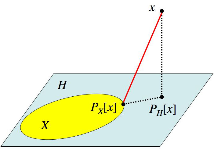
Figure 4: Projection on a set $X$ contained in an affine set $H$.

Now, we are ready to present the result relating the values ${\rm dist}^{2}(x,C(\eta))$ and ${\rm dist}^{2}(x,X_{i}(\eta))$.

Lemma 1

Let $<N,\eta>$ be a TU game with a nonempty core $C(\eta)$. Then, there is a constant $\mu>0$ such that

$${\rm dist}^{2}(x,C(\eta))\leq\mu\sum_{i=1}^{n}{\rm dist}^{2}(x,X_{i}(\eta))\qquad\hbox{for all $x\in\mathbb{R}^{n}$},$$

where $\mu$ depends on the collection of vectors $\{\tilde{e}_{S}\mid S\subset N,\ S\neq\emptyset\}$, where each $\tilde{e}_{S}$ is the projection of $e_{S}$ on the hyperplane $H=\{x\in\mathbb{R}^{n}\mid e_{N}^{\prime}x=\eta_{N}\}$.

Proof. Since the hyperplane $H$ contains the core $C(\eta)$ (see (2)), by relation (10) we have

$${\rm dist}^{2}(x,C(\eta))=\|x-P_{H}[x]\|^{2}+{\rm dist}^{2}(P_{H}[x],C(\eta))\qquad\hbox{for all $x\in\mathbb{R}^{n}$}.$$ (11)

The point $P_{H}[x]$ and the core $C(\eta)$ lie in the $n-1$-dimensional affine set $H$. By applying the Hoffman bound relative to the affine set $H$ (cf. Eq. (9)), we obtain

$${\rm dist}(P_{H}[x],C(\eta))\leq c\,\sum_{S\subset N}{\rm dist}(P_{H}[x],H\cap H_{S}),$$

where the summation is over nonempty subsets $S$, $H_{S}=\{x\in\mathbb{R}^{n}\mid e_{S}^{\prime}x\geq\eta_{S}\}$, while the constant $c$ depends on the collection $\{\tilde{e}_{S},S\subset N\}$ of projections of vectors $e_{S}$ on the hyperplane $H$ for $S\subset N$. Thus, it follows

$${\rm dist}^{2}(P_{H}[x],C(\eta)) \leq c^{2}\,\left(\sum_{S\subset N}{\rm dist}(P_{H}[x],H\cap H_{S})\right)^{2}$$ (12)

$$\leq c^{2}(m-1)\,\sum_{S\subset N}{\rm dist}^{2}(P_{H}[x],H\cap H_{S}),$$ (13)

where $m$ is the number of nonempty subsets of $N$ and the last inequality follows by $(\sum_{j=1}^{\ell}a_{j})^{2}\leq\ell\sum_{j=1}^{\ell}a_{j}^{2}$, which is valid for any finite collection of scalars $a_{j},j=1,\ldots,\ell$ with $\ell\geq 1$. Combining Eq. (12) with equality (11), we obtain for any $x\in\mathbb{R}^{n}$,

$${\rm dist}^{2}(x,C(\eta)) \leq \|x-P_{H}[x]\|^{2}+c^{2}(m-1)\,\sum_{S\subset N}{\rm dist}^{2}(P_{H}[x],H\cap H_{S})$$

$$\leq c_{1}\,\sum_{S\subset N}\left(\|x-P_{H}[x]\|^{2}+{\rm dist}^{2}(P_{H}[x],H\cap H_{S})\right),$$

where $c_{1}=\max\{1,\ c^{2}(m-1)\}$. Since the set $H$ is affine, in view of relation (10) we have $\|x-P_{H}[x]\|^{2}+{\rm dist}^{2}(P_{H}[x],H\cap H_{S})={\rm dist}^{2}(x,H\cap H_{S})$, implying that for any $x\in\mathbb{R}^{n}$,

$${\rm dist}^{2}(x,C(\eta))\leq c_{1}\,\sum_{S\subset N}{\rm dist}^{2}(x,H\cap H_{S}).$$

From the preceding relation, it follows for any $x\in\mathbb{R}^{n},$

$${\rm dist}^{2}(x,C(\eta))\leq c_{1}\sum_{S\subset N}|S|\,{\rm dist}^{2}(x,H\cap H_{S}),$$ (14)

where $|S|$ denotes the cardinality of the coalition $S$. Note that

$$\sum_{S\subset N}|S|\,{\rm dist}^{2}(x,H\cap H_{S}) =\sum_{S\subset N}\sum_{i\in S}\,{\rm dist}^{2}(x,H\cap H_{S})$$ (15)

$$=\sum_{i=1}^{n}\left(\sum_{\{S\subset N\mid i\in S\}}{\rm dist}^{2}(x,H\cap H_{S})\right).$$ (16)

We also note that $X_{i}(\eta)\subset H\cap H_{S}$ for each nonempty $S\subset N$ and $i\in S$, which follows by the definition of $H_{S}$ and relation (1). Furthermore, since ${\rm dist}(x,Y)\leq{\rm dist}(x,X)$ for any $x\in\mathbb{R}^{n}$ and for any two closed convex sets $X,Y\subseteq\mathbb{R}^{n}$ such that $X\subset Y$, it follows that for all $x\in\mathbb{R}^{n}$,

$${\rm dist}(x,H\cap H_{S})\leq{\rm dist}(x,X_{i}(\eta)).$$ (17)

By combining relations (14)–(17), we obtain

$${\rm dist}^{2}(x,C(\eta)) \leq c_{1}\,\sum_{i=1}^{n}\left(\sum_{\{S\subset N\mid i\in S\}}{\rm dist}^{2}(x,X_{i}(\eta))\right)$$

$$= c_{1}\kappa\,\sum_{i=1}^{n}{\rm dist}^{2}(x,X_{i}(\eta)),$$

where $\kappa$ is the number of coalitions $S$ that contain player $i$, which is the same number for every player ($\kappa$ does not depend on $i$). The desired relation follows by letting $\mu=c_{1}\kappa$, and by recalling that $c_{1}=\max\{1,c^{2}(m-1)\}$ and that $c$ depends on the projections $\tilde{e}_{S}$ of vectors $e_{S},S\subset N$, on the hyperplane $H$.   

Note that the scalar $\mu$ in Lemma 1 does not depend on the coalitions’ values $\eta_{S}$ for $S\neq N$. It depends only on the vectors $e_{S}$, $S\subseteq N$, and the grand coalition value $\eta_{N}$.

As a direct consequence of Lemma 1, we have the following result for the instantaneous game $<N,v(t)>$ under the assumptions of Section 2.1.

Lemma 2

Let Assumptions 1 and 2 hold. We then have for all $t\geq 0$,

$${\rm dist}^{2}(x,C(v(t)))\leq\mu\sum_{i=1}^{n}{\rm dist}^{2}(x,X_{i}(t))\qquad\hbox{for all }x\in\mathbb{R}^{n},$$

where $C(v(t))$ is the core of the game $<N,v(t)>$, $X_{i}(t)$ is the bounding set of player $i$, and $\mu$ is the constant from Lemma 1.

Proof. By Assumption 2, we have that the core $C(v^{\max})$ is nonempty. Furthermore, under Assumption 1, we have $C(v^{\max})\subseteq C(v(t))$ for all $t\geq 0$, implying that the core $C(v(t))$ is nonempty for all $t\geq 0$.

Under Assumption 1, each core $C(v(t))$ is defined by the same affine equality corresponding to the grand coalition value, $e_{N}^{\prime}x=v_{N}^{\max}$. Moreover, each core $C(v(t))$ is defined through the set of hyperplanes $H_{S}(t)=\{x\in\mathbb{R}^{n}\mid e_{S}^{\prime}x\geq v_{S}(t)\}$, $S\subset N$, which have time invariant normal vectors $e_{S}$, $S\subseteq N$. Thus, the result follows from Lemma 1.   

3 Convergence to Core of Robust Game

In this section, we prove convergence of the bargaining process in (6) to a random allocation that lies in the core of the robust game with probability 1. We find it convenient to re-write the bargaining protocol (6) by isolating a linear and a non-linear term. The linear term is the vector $w^{i}(t)$ defined as:

$$w^{i}(t)=\sum_{j=1}^{n}a_{ij}(t)x^{j}(t)\qquad\hbox{for all $i\in N$ and $t\geq 0$}.$$ (18)

Note that $w^{i}(t)$ is linear in players’ allocations $x^{j}(t)$. The non-linear term is the error

$$e^{i}(t)=P_{X_{i}(t)}[w^{i}(t)]-w^{i}(t).$$ (19)

Now, using (18) and (19), we can rewrite protocol (6) as follows:

$$x^{i}(t+1)=w^{i}(t)+e^{i}(t)\qquad\hbox{for all $i\in N$ and $t\geq 0$}.$$ (20)

Recall that the weights $a_{ij}(t)$ are nonnegative and such that $a_{ij}(t)=0$ for all $j\not\in\mathcal{N}_{i}(t)$. Also, recall that $A(t)$ is the matrix with entries $a_{ij}(t)$, which governs the construction of the vectors $w^{i}(t)$ in (18).

The main result of this section shows that, with probability 1, the bargaining protocol (18)–(20) converges to the core $C(v^{\max})$ of the robust game $<N,v^{\rm max}>$, provided that $v(t)=v^{\max}$ happens infinitely often in time with probability 1. To establish this we use some auxiliary results, which we develop in the next two lemmas.

The following lemma provides a result on the sequences $x^{i}(t)$ and shows that the errors $e^{i}(t)$ are diminishing.

Lemma 3

Let Assumptions 1 and 2 hold. Also, assume that each matrix $A(t)$ is doubly stochastic. Then, for the bargaining protocol (18)–(20), we have

• The sequence $\left\{\sum_{i=1}^{n}\|x^{i}(t+1)-x\|^{2}\right\}$ converges for every $x\in C(v^{\max})$.

• The errors $e^{i}(t)$ in (19) are such that $\sum_{t=0}^{\infty}\sum_{j=1}^{n}\|e^{i}(t)\|^{2}<\infty$. In particular, $\lim_{t\to\infty}\|e^{i}(t)\|=0$ for all $i\in N$.

Proof. By $x^{i}(t+1)=P_{X_{i}(t)}[w^{i}(t)]$ and by strictly non-expansive property of the Euclidean projection on a closed convex set $X_{i}(t)$ (see (8)), we have for any $i\in N$, $t\geq 0$ and $x\in X_{i}(t)$,

$$\|x^{i}(t+1)-x\|^{2}\leq\|w^{i}(t)-x\|^{2}-\|e^{i}(t)\|^{2}.$$ (21)

Under Assumptions 1 and 2, the core $C(v^{\rm max})$ is contained in the core $C(v(t))$ for all $t\geq 0$, implying that $C(v^{\max})\subseteq C(v(t))$ for all $t\geq 0$. Furthermore, since $C(v(t))=\cap_{i=1}^{n}X_{i}(t)$, it follows that $C(v^{\max})\subseteq X_{i}(t)$ for all $i\in N$ and $t\geq 0$. Therefore, relation (21) holds for all $x\in C(v^{\max})$. Thus, by summing the relations in (21) over $i\in N$, we obtain for all $t\geq 0$ and $x\in C(v^{\max})$,

$$\sum_{i=1}^{n}\|x^{i}(t+1)-x\|^{2}\leq\sum_{i=1}^{n}\|w^{i}(t)-x\|^{2}-\sum_{i=1}^{n}\|e^{i}(t)\|^{2}.$$ (22)

By the definition of $w^{i}(t)$ in (18), using the stochasticity of $A(t)$ and the convexity of the squared norm, we obtain

$$\sum_{i=1}^{n}\|w^{i}(t)-x\|^{2}=\sum_{i=1}^{n}\left\|\sum_{j=1}^{n}a_{ij}(t)x^{j}(t)-x\right\|^{2}\leq\sum_{j=1}^{n}\left(\sum_{i=1}^{n}a_{ij}(t)\right)\|x^{j}(t)-x\|^{2}.$$

By the doubly stochasticity of $A(t)$, we have $\sum_{i=1}^{n}a_{ij}(t)=1$ for every $j$, implying $\sum_{i=1}^{n}\|w^{i}(t)-x\|^{2}\leq\sum_{i=1}^{n}\|x^{i}(t)-x\|^{2}$. By substituting this relation in (22), we arrive at

$$\sum_{i=1}^{n}\|x^{i}(t+1)-x\|^{2}\leq\sum_{i=1}^{n}\|x^{i}(t)-x\|^{2}-\sum_{i=1}^{n}\|e^{i}(t)\|^{2}.$$ (23)

The preceding relation shows that the scalar sequence $\{\sum_{i=1}^{n}\|x^{i}(t+1)-x\|^{2}\}$ is non-increasing for any given $x\in C(v^{\max})$. Therefore, the sequence must be convergent since it is nonnegative. Moreover, by summing the relations in (23) over $t=0,\ldots,s$ and taking the limit as $s\rightarrow\infty$, we obtain

$$\sum_{t=0}^{\infty}\sum_{i=1}^{n}\|e^{i}(t)\|^{2}\leq\sum_{i=1}^{n}\|x^{i}(0)-x\|^{2},$$

which implies that $\lim_{t\to\infty}e^{i}(t)=0$ for all $i\in N$.   

In our next result, we will use the instantaneous average of players allocations, defined as follows:

$$y(t)=\frac{1}{n}\sum_{j=1}^{n}x^{j}(t)\qquad\hbox{for all }t\geq 0.$$

The result shows that the difference between the bargaining payoff vector $x^{i}(t)$ for any player $i$ and the average $y(t)$ of these payoffs converges to 0 as time goes to infinity. The proof essentially uses the line of analysis that has been employed in [17], where the sets $X_{i}(t)$ are static in time, i.e., $X_{i}(t)=X_{i}$ for all $t$. In addition, we also use the rate result for doubly stochastic matrices that has been established in [15].

Lemma 4

Let Assumptions 3 and 4 hold. Suppose that for the bargaining protocol (18)–(20) we have

$$\lim_{t\to\infty}\|e^{i}(t)\|=0\qquad\hbox{for all }i\in N.$$

Then, for every player $i\in N$ we have

$$\lim_{t\to\infty}\|x^{i}(t)-y(t)\|=0,\qquad\lim_{t\to\infty}\|w^{i}(t)-y(t)\|=0.$$

Proof. For any $t\geq s\geq 0$, define matrices

$$\Phi(t,s)=A(t)A(t-1)\cdots A(s+1)A(s),$$

with $\Phi(t,t)=A(t)$. Using the matrices $\Phi(t,s)$ and the expression for $x^{i}(t)$ in (20), we can relate the vectors $x^{i}(t)$ with the vectors $x^{i}(s)$ at a time $s$ for $0\leq s\leq t-1$, as follows:

$$x^{i}(t)=\sum_{j=1}^{n}[\Phi(t-1,s)]_{ij}\,x^{j}(s)+\sum_{r=s+1}^{t-1}\left(\sum_{j=1}^{n}[\Phi(t-1,r)]_{ij}\,e^{j}(r-1)\right)+e^{i}(t-1).$$ (24)

Under the doubly stochasticity of the matrices $A(t)$, using $y(t)=\frac{1}{n}\sum_{j=1}^{n}x^{j}(t)$ and relation (24), we obtain

$$y(t)={1\over n}\sum_{j=1}^{n}x^{j}(s)+{1\over n}\sum_{r=s+1}^{t}\left(\sum_{j=1}^{n}e^{j}(r-1)\right)\qquad\hbox{for all $t\geq s\geq 0$}.$$ (25)

By our assumption, we have $\lim_{t\to\infty}\|e^{i}(t)\|=0$ for all $i$. Thus, for any $\epsilon>0$, there is an integer $\hat{s}\geq 0$ such that $\|e^{i}(t)\|\leq\epsilon$ for all $t\geq\hat{s}$ and all $i$. Using relations (24) and (25) with $s=\hat{s}$, we obtain for all $i$ and $t\geq\hat{s}+1$,

$$\|x^{i}(t)-y(t)\|=\left\|\sum_{j=1}^{n}\Big{(}[\Phi(t-1,\hat{s})]_{ij}-{1\over n}\Big{)}x^{j}(\hat{s})\right.$$

$$+ \left.\sum_{r=\hat{s}+1}^{t-1}\sum_{j=1}^{n}\Big{(}[\Phi(t-1,r)]_{ij}-{1\over n}\Big{)}e^{j}(r-1)+\Big{(}e^{i}(t-1)-{1\over n}\sum_{j=1}^{n}e^{j}(t-1)\Big{)}\right\|$$

$$\leq \sum_{j=1}^{n}\Big{|}[\Phi(t-1,\hat{s})]_{ij}-{1\over n}\Big{|}\ \|x^{j}(\hat{s})\|$$

$$+ \sum_{r=\hat{s}+1}^{t-1}\sum_{j=1}^{n}\Big{|}[\Phi(t-1,r)]_{ij}-{1\over n}\Big{|}\|e^{j}(r-1)\|+\|e^{i}(t-1)\|+{1\over n}\sum_{j=1}^{n}\|e^{j}(t-1)\|.$$

Since $\|e^{i}(t)\|\leq\epsilon$ for all $t\geq\hat{s}$ and all $i$, it follows that

$$\|x^{i}(t)-y(t)\|\leq\sum_{j=1}^{n}\Big{|}[\Phi(t-1,\hat{s})]_{ij}-{1\over n}\Big{|}\ \|x^{j}(\hat{s})\|+\epsilon\sum_{r=\hat{s}+1}^{t-1}\sum_{j=1}^{n}\Big{|}[\Phi(t-1,r)]_{ij}-{1\over n}\Big{|}\ +2\epsilon.$$

Under Assumptions 3 and 4, the following result holds for the matrices $\Phi(t,s)$, as shown in [14] (see there Corollary 1):

$$\left|[\Phi(t,s)]_{ij}-\frac{1}{n}\right|\leq\left(1-\frac{\alpha}{4n^{2}}\right)^{\left\lceil\frac{t-s+1}{Q}\right\rceil-2}\qquad\hbox{for all }t\geq s\geq 0.$$

Substituting the preceding estimate in the estimate for $\|x^{i}(t)-y(t)\|$, we obtain

$$\|x^{i}(t)-y(t)\|\leq\left(1-\frac{\alpha}{4n^{2}}\right)^{\left\lceil\frac{t-\hat{s}}{Q}\right\rceil-2}\sum_{j=1}^{n}\|x^{j}(\hat{s})\|+n\epsilon\sum_{r=\hat{s}+1}^{t-1}\left(1-\frac{\alpha}{4n^{2}}\right)^{\left\lceil\frac{t-r}{Q}\right\rceil-2}\,+2\epsilon.$$

Letting $t\to\infty$, we see that

$$\limsup_{t\to\infty}\|x^{i}(t)-y(t)\|\leq n\epsilon\sum_{r=\hat{s}+1}^{\infty}\left(1-\frac{\alpha}{4n^{2}}\right)^{\left\lceil\frac{t-r}{Q}\right\rceil-2}+2\epsilon.$$

Note that $\sum_{r=\hat{s}+1}^{\infty}\left(1-\frac{\alpha}{4n^{2}}\right)^{\left\lceil\frac{t-r}{Q}\right\rceil-2}<\infty$, which by the arbitrary choice of $\epsilon$ yields

$$\lim_{t\to\infty}\|x^{i}(t)-y(t)\|=0\qquad\hbox{for all $i\in N$}.$$

Now, we focus on $\sum_{i=1}^{n}\|w^{i}(t)-y(t)\|$. Since $w^{i}(t)=\sum_{j=1}^{n}a_{ij}(t)x^{j}(t)$ and since $A(t)$ is stochastic, it follows

$$\sum_{i=1}^{n}\|w^{i}(t)-y(t)\|\leq\sum_{i=1}^{n}\sum_{j=1}^{n}a_{ij}(t)\|x^{j}(t)-y(t)\|.$$

Exchanging the order of the summations over, and then using the doubly stochasticity of $A(t)$, we have

$$\sum_{i=1}^{n}\|w^{i}(t)-y(t)\|\leq\sum_{j=1}^{n}\left(\sum_{i=1}^{n}a_{ij}(t)\right)\|x^{j}(t)-y(t)\|=\sum_{j=1}^{n}\|x^{j}(t)-y(t)\|.$$

Since $\lim_{t\to\infty}\|x^{j}(t)-y(t)\|=0$ for all $j$, it follows that $\sum_{i=1}^{n}\|w^{i}(t)-y(t)\|\to 0,$ thus implying $\|w^{i}(t)-y(t)\|\to 0$ for all $i\in N$.   

Note that Lemma 4 captures the effects of the matrices $A(t)$ that represent players’ neighbor-graphs. At the same time, Lemma 3 is basically a consequence of the projection property only. So far, the polyhedrality of the sets $X_{i}(t)$ has not been used at all. We now put all pieces together, namely Lemma 2 that exploits the polyhedrality of the bounding sets $X_{i}(t)$, Lemma 3 and Lemma 4. This brings us to the following convergence result for the robust game $<N,v^{\rm max}>$.

Theorem 1

Let Assumptions 1–4 hold. Also, assume that

$${\rm Prob}\,\left\{v(t)=v^{\max}\ \ i.o.\right\}=1,$$

where $i.o.$ stands for infinitely often. Then, the players allocations $x^{i}(t)$ generated by bargaining protocol (18)–(20) converge with probability 1 to an allocation in the core $C(v^{\max})$, i.e., there is a random vector $\tilde{x}\in C(v^{\max})$ such that with probability 1,

$$\lim_{t\rightarrow\infty}\|x^{i}(t)-\tilde{x}\|=0\qquad\mbox{for all $i\in N$}.$$

Proof. By Lemma 3, for each player $i\in N$, the sequence $\{\sum_{i=1}^{n}\|x^{i}(t)-x\|^{2}\}$ is convergent for every $x\in C(v^{\max})$ and the errors $e^{i}(t)$ are diminishing, i.e., $\|e^{i}(t)\|\to 0$. Then, by Lemma 4 we have $\|x^{i}(t)-y(t)\|\to 0$ for every $i$. Hence,

$$\hbox{$\{\|y(t)-x\|\}$ is convergent for every $x\in C(v^{\max})$}.$$ (26)

We want to show that $\{y(t)\}$ is convergent and that its limit is in the core $C(v^{\max})$ with probability 1. For this, we note that since $x^{i}(t+1)\in X_{i}(t)$, it holds

$$\sum_{i=1}^{n}{\rm dist}^{2}\left(y(t+1),X_{i}(t)\right)\leq\sum_{i=1}^{n}\|y(t+1)-x^{i}(t+1)\|^{2}\qquad\hbox{for all $t\geq 0$}.$$

The preceding relation and $\|x^{i}(t)-y(t)\|\rightarrow 0$ for all $i\in N$ (cf. Lemma 4) imply

$$\lim_{t\rightarrow\infty}\sum_{i=1}^{n}{\rm dist}^{2}\left(y(t+1),X_{i}(t)\right)=0.$$

Under Assumptions 1 and 2, by Lemma 2 we obtain

$${\rm dist}^{2}\left(y(t+1),C(v(t))\right)\leq\mu\sum_{i=1}^{n}{\rm dist}^{2}\left(y(t+1),X_{i}(t)\right)\qquad\hbox{for all $t\geq 0$}.$$

By combining the preceding two relations we see that

$$\lim_{t\to\infty}\,{\rm dist}^{2}\left(y(t+1),C(v(t))\right)=0.$$ (27)

By our assumption, the event $\{v(t)=v^{\max}\ \hbox{infinitely often}\}$ happens with probability 1. We now fix a realization $\{v_{\omega}(t)\}$ of the sequence $\{v(t)\}$ such that $v_{\omega}(t)=v^{\max}$ holds infinitely often (for infinitely many $t$’s). Let $\{t_{k}\}$ be a sequence such that

$$v_{\omega}(t_{k})=v^{\max}\qquad\hbox{for all }k.$$

All the variables corresponding to the realization $\{v_{\omega}(t)\}$ are denoted by a subscript $\omega$. By relation (26) the sequence $\{y_{\omega}(t)\}$ is bounded, therefore $\{y_{\omega}(t_{k})\}$ is bounded. Without loss of generality (by passing to a subsequence of $\{t_{k}\}$ if necessary), we assume that $\{y_{\omega}(t_{k})\}$ converges to some vector $\tilde{y}_{\omega}$, i.e.,

$$\lim_{k\to\infty}y_{\omega}(t_{k})=\tilde{y}_{\omega}.$$

Thus, the preceding two relations and Eq. (27) imply that $\tilde{y}_{\omega}\in C(v^{\max})$. Then, by relation (26), we have that $\{\|y_{\omega}(t)-\tilde{y}_{\omega}\|\}$ is convergent, from which we conclude that $\tilde{y}_{\omega}$ must be the unique accumulation point of the sequence $\{y_{\omega}(t)\}$, i.e.,

$$\lim_{t\to\infty}y_{\omega}(t)=\tilde{y}_{\omega},\qquad\tilde{y}_{\omega}\in C(v^{\max}).$$

This and the assumption ${\rm Prob}\,\left\{v(t)=v^{\max}\ \ i.o.\right\}=1,$ imply that the sequence $\{y(t)\}$ converges with probability 1 to a random point $\tilde{y}\in C(v^{\max})$. Since by Lemma 4 we have $\|x^{i}(t)-y(t)\|\to 0$ for every $i$, it follows that the sequences $\{x^{i}(t)\},i=1,\ldots,n,$ converge with probability 1 to a common random point in the core $C(v^{\max})$.  

4 Dynamic Average Game

When the core of the robust game is empty, the core of the instantaneous average game can provide a meaningful solution under some conditions on the distribution of the functions $v(t)$. In what follows, we focus on the instantaneous average game associated with the dynamic TU game $<N,\{v(t)\}>$. In the next sections, we define the instantaneous average game, we introduce a bargaining protocol for the game and investigate the convergence properties of the bargaining protocol.

4.1 Average Game and Bargaining Protocol

Consider a dynamic TU game $<N,\{v(t)\}>$ with each $v(t)$ being a random characteristic function. With the dynamic game we associate a dynamic average game $<N,\{\bar{v}(t)\}>$, where $\bar{v}(t)$ is the average of the characteristic functions $v(0),\ldots,v(t)$, i.e.,

$$\bar{v}(t)=\frac{1}{t+1}\,\sum_{k=0}^{t}v(k)\qquad\hbox{for all }t\geq 0.$$

An instantaneous average game at time $t\geq 0$ is the game $<N,\bar{v}(t)>$. We let $C(\bar{v}(t))$ denote the core of the instantaneous average game at time $t$ and let $\bar{X}_{i}(t)$ denote the bounding set of player $i$ for the instantaneous game $<N,\bar{v}(t)>$, i.e., for all $i\in N$ and $t\geq 0$,

$$\bar{X}_{i}(t)=\left\{x\in\mathbb{R}^{n}\mid e_{N}^{\prime}x=\bar{v}_{N}(t),\ e_{S}^{\prime}x\geq\bar{v}_{S}(t)\mbox{ for all $S\subset N$ such that $i\in S$}\right\}.$$ (28)

Note that $\bar{X}_{i}(0)=X_{i}(0)$ for all $i\in N$ since $\bar{v}(0)=v(0)$. In what follows, we assume that $\bar{X}_{i}(t)$ are nonempty for all $i\in N$ and all $t\geq 0$.

In this setting, the bargaining process for the players is given by

$$x^{i}(t+1)=P_{\bar{X}_{i}(t)}\left[\sum_{j=1}^{n}a_{ij}(t)x^{j}(t)\right]\qquad\hbox{for all $i\in N$ and $t\geq 0$},$$ (29)

where $a_{ij}(t)\geq 0$ is a scalar weight that player $i$ assigns to the proposed allocation $x^{j}(t)$ received from player $j$ at time $t$. The initial allocations $x^{i}(0)$, $i\in N$, are selected randomly and independently of $\{v(t)\}$. Regarding the weights $a_{ij}(t)$, recall that these weights are reflective of the players’ neighbor-graph: $a_{ij}(t)=0$ for all $j\not\in\mathcal{N}_{i}(t)$, where $\mathcal{N}_{i}(t)$ is the set of neighbors of player $i$ (including himself) at time $t$, while we may have $a_{ij}(t)\geq 0$ only for $j\in\mathcal{N}_{i}(t)$.

4.2 Assumptions and Preliminaries

In this section, we provide our assumptions for the average game, and discuss some auxiliary results that we need later on in the convergence analysis of the bargaining protocol. Regarding the random characteristic functions $v(t)$ we use the following assumption.

Assumption 5

The sequence $\{v(t)\}$ is ergodic, i.e., with probability 1, we have

$$\lim_{t\to\infty}\bar{v}(t)=v^{\rm mean}\qquad\hbox{with $v^{\rm mean}\in\mathbb{R}^{m}$}.$$

Furthermore, $v_{N}(t)=v^{\rm mean}$ for all $t$ with probability 1.

Assumption 5 basically says that the grand coalition value $v_{N}(t)$ is constant with probability 1. Note that Assumption 5 is satisfied, for example, when $\{v_{S}(t)\}$ is an independent identically distributed sequence with a finite expectation $\mathsf{E}\!\left[v_{S}(t)\right]$ for all $S\subset N$.

We refer to the TU game $<N,v^{\rm mean}>$ as average game, which is well defined under Assumption 5. We let $C(v^{\rm mean})$ be the core of the average game and $\bar{X}_{i}$ be the bounding set for player $i$ in the game, i.e.,

$$C(v^{\rm mean})=\left\{x\in\mathbb{R}^{n}\mid e_{N}^{\prime}x=v^{\rm mean}_{N},\ e_{S}^{\prime}x\geq v^{\rm mean}_{S}\quad\hbox{for all nonempty $S\subset N$}\right\},$$

$$\bar{X}_{i}=\left\{x\in\mathbb{R}^{n}\mid e_{N}^{\prime}x=v^{\rm mean}_{N},\ e_{S}^{\prime}x\geq v^{\rm mean}_{S}\quad\hbox{for all $S\subset N$ such that $i\in S$}\right\}.$$ (30)

Note that the average core $C(v^{\rm mean})$ lies in the hyperplane $H=\{x\in\mathbb{R}^{n}\mid e_{N}^{\prime}x=v^{\rm mean}_{N}\}$. Hence, the dimension of the core is at most $n-1$. We will in fact assume that the dimension of the average core $C(v^{\rm mean})$ is $n-1$, by requiring the existence of a point $z$ in the core such that all other inequalities defining the core are satisfied as strict inequalities.

Specifically, we make use of the following assumption.

Assumption 6

There exists a vector $\hat{z}\in C(v^{\rm mean})$ such that

$$e_{S}^{\prime}\hat{z}>v^{\rm mean}_{S}\qquad\hbox{for all nonempty }S\subset N.$$

Assumption 6 basically says that $\hat{z}$ is in the relative interior of the core $C(v^{\rm mean})$ of the average game and that the core $C(v^{\rm mean})$ has dimension $n-1$. This assumption will be important in establishing the convergence of the bargaining protocol (29). In particular, the following result will be important, which is an immediate consequence of Assumption 6 and the polyhedrality of the cores $C(\bar{v}(t))$.

Lemma 5

Let Assumptions 5 and 6 hold. Then, with probability 1, for every $z$ in relative interior of $C(v^{\rm mean})$ there exists $t_{z}$ large enough such that $z$ is in the relative interior of $C(\bar{v}(t))$ for all $t\geq t_{z}$ with probability 1.

Proof. Let $z$ be in the relative interior of $C(v^{\rm mean})$ which exists by Assumption 6. Thus, $e_{N}^{\prime}z=v^{\rm mean}_{N}$ and $e_{S}^{\prime}z>v^{\rm mean}_{S}$ for all $S\subset N$. By Assumption 5, with probability 1 we have $\bar{v}_{N}(t)=v^{\rm mean}_{N}$ and $\bar{v}_{S}(t)\to v^{\rm mean}_{S}$ for $S\subset N$. Hence, $\bar{v}_{N}(t)^{\prime}z=(v^{\rm mean}_{N})^{\prime}z$ for all $t$ with probability 1. Furthermore, there exists a random time $t_{z}$ large enough so that with probability 1,

$$e_{S}^{\prime}z>\bar{v}_{S}(t)\qquad\hbox{for all $S\subset N$ and all $t\geq t_{z}$},$$

implying that $z$ is in the relative interior of $C(\bar{v}(t))$ for all $t\geq t_{z}$ with probability 1.    Lemma 5 shows that the sets $C(\bar{v}(t))$ and $C(v^{\rm mean})$ have the same dimension for large enough $t$ with probability 1. In particular, this lemma implies that the cores $C(\bar{v}(t))$ are nonempty with probability 1 for all $t$ sufficiently large.

Aside from Lemma 5, in our convergence analysis of the bargaining protocol, we make use of two additional well-known results. One of them is the super-martingale convergence theorem due to Robbins and Siegmund [21] (it can also be found in [18], Chapter 2.2, Lemma 11).

Theorem 2

Let $\{V_{k}\},\{g_{k}\},$ and $\{h_{k}\}$ be non-negative random scalar sequences. Let $F_{k}$ be the $\sigma$-algebra generated by $V_{1},\ldots,V_{k},g_{1},\ldots g_{k},h_{1},\ldots h_{k}.$ Suppose that almost surely,

$$\mathsf{E}\!\left[V_{k+1}\mid F_{k}\right]\leq V_{k}-g_{k}+h_{k}\qquad\hbox{for all $k$,}$$

and $\sum_{k}h_{k}<\infty$ almost surely. Then, almost surely both the sequence $\{V_{k}\}$ converges to a non-negative random variable and $\sum_{k}g_{k}<\infty$.

The other well-known result that we use is pertinent to two nonempty polyhedral sets whose description differs only in the right-hand side vector. The result can be found in [7], 3.2.5 Corollary, pages 258–259.

Lemma 6

Let $P_{b}$ and $P_{\tilde{b}}$ be two polyhedral sets given by

$$P_{b}=\{x\in\mathbb{R}^{n}\mid Bx\leq b\},\qquad P_{\tilde{b}}=\{x\in\mathbb{R}^{n}\mid Bx\leq\tilde{b}\},$$

where $B$ is an $m\times n$ matrix and $b,\tilde{b}\in\mathbb{R}^{m}$. Then, there is a scalar $L>0$ such that for every $b,\tilde{b}\in\mathbb{R}^{m}$ for which $P_{b}\neq\emptyset$ and $P_{\tilde{b}}\neq\emptyset$, we have

$${\rm dist}(x,P_{\tilde{b}})\leq L\|b-\tilde{b}\|\qquad\hbox{for any $x\in P_{b}$,}$$

where the constant $L$ depends on the matrix $B$.

For two polyhedral sets $P_{b}$ and $P_{\tilde{b}}$ as in Lemma 6 we also have

$${\rm dist}(x,P_{b})\leq{\rm dist}(x,P_{\tilde{b}})+L\|b-\tilde{b}\|\qquad\hbox{for any }x\in\mathbb{R}^{n}$$ (31)

(see Rockafellar [22], 4.34 Lemma on page 132).

4.3 Convergence to Core of Average Game

Here, we show the convergence of the bargaining protocol to the core of the average game. In our analysis, we find it convenient to re-write the bargaining protocol (29) in an equivalent form by separating a linear and a non-linear term. The linear term is the vector $\bar{w}^{i}(t)$ given by

$$\bar{w}^{i}(t)=\sum_{j=1}^{n}a_{ij}(t)x^{j}(t)\qquad\hbox{for all $i\in N$ and $t$}.$$ (32)

The non-linear term is expressed by the error

$$\bar{e}^{i}(t)=P_{\bar{X}_{i}(t)}[\bar{w}^{i}(t)]-\bar{w}^{i}(t).$$ (33)

Now, using relations (32) and (33), we can rewrite (29) as follows:

$$x^{i}(t+1)=\bar{w}^{i}(t)+\bar{e}^{i}(t)\qquad\hbox{for all $i\in N$ and all $t\geq 0$}.$$ (34)

We first show some basic properties of the players’ allocations by using the preceding equivalent description of the bargaining protocol (29). These properties hold under the doubly stochasticity of the weights $a_{ij}(t)$ that comprise the matrix $A(t)$.

Lemma 7

Let Assumptions 5 and 6 hold. Also, let the matrices $A(t)$ be doubly stochastic. Then, for bargaining protocol (32)–(34), we have with probability 1:

• The sequence $\{\sum_{i=1}^{n}\|x^{i}(t+1)-z\|^{2}\}$ converges for every $z$ in the relative interior of $C(v^{\rm mean})$.

• The errors $\bar{e}^{i}(t)$ in (19) are such that $\sum_{t=0}^{\infty}\sum_{j=1}^{n}\|\bar{e}^{i}(t)\|^{2}<\infty$. In particular, $\lim_{t\to\infty}\|\bar{e}^{i}(t)\|=0$ for all $i\in N$.

Proof. Let ${\rm rint}Y$ denote the relative interior of a set $Y$. Let $z\in{\rm rint}C(v^{\rm mean})$ be arbitrary and fixed for the rest of the proof. By Lemma 5, there exists $t_{z}$ large enough such that $z\in{\rm rint}C(\bar{v}(t))$ for all $t\geq t_{z}$ with probability 1. Since $C(\bar{v}(t))=\cap_{i=1}^{n}X_{i}(t)$, it follows that $z\in\bar{X}_{i}(t)$ for all $i\in N$ and $t\geq t_{z}$ with probability 1.

From $x^{i}(t+1)=\bar{w}^{i}(t)+\bar{e}^{i}(t)$ (cf. (34)), the definition of $\bar{e}^{i}(t)$ in (33), and the projection property given in Eq. (8), we have with probability 1, for $i\in N$ and all $t\geq t_{z}$,

$$\|x^{i}(t+1)-z\|^{2}\leq\|\bar{w}^{i}(t)-z\|^{2}-\|\bar{e}^{i}(t)\|^{2}.$$

Summing these relations over $i\in N$, and using $\bar{w}^{i}(t)=\sum_{j=1}^{n}a_{ij}x^{i}(t)$, the convexity of the norm and the stochasticity of $A(t)$, we obtain

$$\sum_{i=1}^{n}\|x^{i}(t+1)-z\|^{2}\leq\sum_{i=1}^{n}\sum_{j=1}^{n}a_{ij}(t)\|x^{j}(t)-z\|^{2}-\sum_{j=1}^{n}\|\bar{e}^{i}(t)\|^{2}.$$

Exchanging the order of summation in $\sum_{i=1}^{n}\sum_{j=1}^{n}a_{ij}(t)\|x^{j}(t)-z\|^{2}$ and using the doubly stochasticity of $A(t)$, we have for all $t\geq t_{z}$ with probability 1,

$$\sum_{i=1}^{n}\|x^{i}(t+1)-z\|^{2}\leq\sum_{j=1}^{n}\|x^{j}(t)-z\|^{2}-\sum_{j=1}^{n}\|\bar{e}^{i}(t)\|^{2}.$$

Applying the super-martingale converge theorem (Theorem 2) (with an index shift), we see that the sequence $\{\sum_{i=1}^{n}\|x^{i}(t+1)-z\|^{2}\}$ is convergent and $\sum_{t=t_{z}}^{\infty}\sum_{j=1}^{n}\|\bar{e}^{i}(t)\|^{2}<\infty$ with probability 1. Hence, the result in part (b) follows.   

We observe that Lemma 4 applies to protocol (32)–(34) in view of the analogy of the description of the protocol in (18)–(20) and the protocol in (32)–(34). We will re-state this lemma for an easier reference, but without the proof since it is almost the same as that of Lemma 4 (the proof in essence depends mainly on the matrices $A(k)$).

Lemma 8

Let Assumptions 3 and 4 hold. Suppose that for the bargaining protocol (32)–(34) we have with probability 1,

$$\lim_{t\to\infty}\|\bar{e}^{i}(t)\|=0\qquad\hbox{for all }i\in N.$$

Then, for every player $i\in N$ we have with probability 1,

$$\lim_{t\to\infty}\|x^{i}(t)-y(t)\|=0,\qquad\lim_{t\to\infty}\|\bar{w}^{i}(t)-y(t)\|=0,$$

where $y(t)=\frac{1}{n}\sum_{j=1}^{n}x^{j}(t)$.

We are now ready to show the convergence of the bargaining protocol. We show this in the following theorem by combining the basic properties of the protocol established in Lemma 7 and using Lemma 8.

Theorem 3

Let Assumptions 3–6 hold. Then, the bargaining protocol (32)–(34) converges to a random allocation that lies in the core $C(v^{\rm mean})$ of the average game with probability 1, i.e., there is a random vector $\tilde{z}\in C(v^{\rm mean})$ such that with probability 1,

$$\lim_{t\rightarrow\infty}\|x^{i}(t)-\tilde{z}\|=0\qquad\mbox{for all $i\in N$}.$$

Proof. By Lemma 7, with probability 1, the sequence $\{\sum_{i=1}^{n}\|x^{i}(t)-z\|^{2}\}$ is convergent for every $z$ in the relative interior of $C(v^{\rm mean})$ and $\|e^{i}(t)\|\to 0$ for each player $i\in N$. By Lemma 8, with probability 1 we have

$$\lim_{t\to\infty}\|x^{i}(t)-y(t)\|=0\qquad\hbox{for every $i\in N$}.$$ (35)

Hence, with probability 1,

$$\hbox{$\{\|y(t)-z\|\}$ is convergent for every $z\in{\rm rint}C(v^{\rm mean})$}.$$ (36)

We next show that $\{y(t)\}$ has accumulation points in the core $C(v^{\rm mean})$ with probability 1. Since $x^{i}(t+1)\in\bar{X}_{i}(t)$, it follows

$$\sum_{i=1}^{n}{\rm dist}^{2}\left(y(t+1),\bar{X}_{i}(t)\right)\leq\sum_{i=1}^{n}\|y(t+1)-x^{i}(t+1)\|^{2}.$$ (37)

Relations (37) and (35) imply

$$\lim_{t\rightarrow\infty}\sum_{i=1}^{n}{\rm dist}^{2}\left(y(t+1),\bar{X}_{i}(t)\right)=0\quad\hbox{with probability~{}1}.$$ (38)

Let $i\in N$ be arbitrary but fixed and let $x\in\bar{X}_{i}$ be arbitrary. Note that we can write

$$\|y(t+1)-x\|\leq\|y(t+1)-P_{\bar{X}_{i}(t)}[y(t+1)]\|+\|P_{\bar{X}_{i}(t)}[y(t+1)]-x\|.$$

By taking the minimum over $x\in\bar{X}_{i}$ and using $\|y(t+1)-P_{\bar{X}_{i}(t)}[y(t+1)]\|={\rm dist}(y(t+1),\bar{X}_{i}(t))$, we obtain for all $i\in N$ and $t\geq 0$,

$${\rm dist}(y(t+1),\bar{X}_{i})\leq{\rm dist}(y(t+1),\bar{X}_{i}(t))+{\rm dist}\left(P_{\bar{X}_{i}(t)}[y(t+1)],\bar{X}_{i}\right).$$

The bounding sets $\bar{X}_{i}$ are nonempty by Assumption 6 and the fact $C(v^{\rm mean})\subset\bar{X}_{i}$ for all $i$, while $\bar{X}_{i}(t)$ are assumed nonempty (see the discussion after relation (28)). Furthermore, since $\bar{X}_{i}$ and $\bar{X}_{i}(t)$ are polyhedral sets, by Lemma 6 it follows that for a scalar $L_{i}>0$ and all $t\geq 0$,

$${\rm dist}\left(P_{\bar{X}_{i}(t)}[y(t+1)],\bar{X}_{i}\right)\leq L_{i}\|\bar{v}(t)-v^{\rm mean}\|.$$

Therefore, for all $i\in N$ and all $t\geq 0$,

$${\rm dist}(y(t+1),\bar{X}_{i})\leq{\rm dist}(y(t+1),\bar{X}_{i}(t))+L_{i}\|\bar{v}(t)-v^{\rm mean}\|.$$

By letting $t\to\infty$ and using relations (38) and $\bar{v}(t)\to v^{\rm mean}$ (Assumption 5), we see that for all $i\in N$ with probability 1,

$$\lim_{t\to\infty}\,{\rm dist}(y(t+1),\bar{X}_{i})=0.$$ (39)

In view of relation (36), the sequence $\{y(t)\}$ is bounded with probability 1, so it has accumulation points with probability 1. By relation (39), all accumulation points of $\{y(t+1)\}$ lie in the set $\bar{X}_{i}$ for every $i\in N$ with probability 1. Therefore, the accumulation points of $\{y(t)\}$ must lie in the intersection $\cap_{i\in N}\bar{X}_{i}$ with probability 1. Since $\cap_{i\in N}\bar{X}_{i}=C(v^{\rm mean})$, we conclude that all accumulation points of $\{y(t)\}$ lie in the core $C(v^{\rm mean})$ with probability 1. Furthermore, according to relation (36) we have that, for any point $z\in{\rm rint}C(v^{\rm mean})$, the accumulation points of the sequences $\{y(t)\}$ are at the same (random) distance from $z$ with probability 1. Since the accumulation points are in the set $C(v^{\rm mean})$, it follows that $\{y(k)\}$ is convergent with probability 1 and its limit point is in the core $C(v^{\rm mean})$ with probability 1. Now, since $\|x^{i}(t)-y(t)\|\to 0$ with probability 1 for all $i$ (see (35)), the sequences $\{x^{i}(t)\}$, $i\in N$, have the same limit point as the sequence $\{y(t)\}$. Thus, the sequences $\{x^{i}(t)\}$, $i\in N$, converge to a common (random) point in $C(v^{\rm mean})$ with probability 1.   

Theorem 3 shows the convergence of the allocations generated by the bargaining protocol in (32)–(34). The convergence relies on the properties of the matrices and the connectivity of the players’ neighbor graphs, as reflected in Assumptions 3 and 4. It also critically depends on the fact that the core of the average game $C(v^{\rm mean})$ has dimension $n-1$ and that all bounding sets $\bar{X}_{i}(t)$ and, hence the cores $C(\bar{v}(t))$, lie in the same hyperplane with probability 1, the hyperplane defined through the constant value of the grand coalition.

5 Numerical Illustrations

In this section, we report some numerical simulations. We consider coalitional TU games with 3 players, so the number of possible nonempty coalitions is $m=7$. We consider two different scenarios as shown respectively in rows I and II in Table 2. The columns of Table 2 enumerate the coalitions. In each scenario, the characteristic functions $v_{S}(t)$ are generated independently with identical uniform distribution over an interval. Specifically, we suppose that the values of single player coalitions $\{1\}$ and $\{2\}$ are uncertain within the given interval. All the other coalitions’ values are fixed and equal to zero except for the grand coalition, which has value 10 in both scenarios I and II.

	$v_{\{1\}}$	$v_{\{2\}}$	$v_{\{3\}}$	$v_{\{1,2\}}$	$v_{\{1,3\}}$	$v_{\{2,3\}}$	$v_{\{1,2,3\}}$
I	$[4,7]$	$[0,3]$	$0$	$0$	$0$	$0$	$10$
II	$[4,9]$	$[0,5]$	$0$	$0$	$0$	$0$	$10$

Table 2: Coalitions’ values for the two simulations scenarios.

The two scenarios differ in that the core $C(v^{\max})$ of the robust game is nonempty in scenario I and empty in scenario II. For scenario I, we simulate the convergence behavior of the bargaining protocol (18)–(20) for the robust game, while for scenario II, we simulate bargaining protocol (32)–(34) for the average game.

Figure 5: Topology of players’ neighbor-graph at three distinct times $t=0$, 1 and 2.

For each scenario, we run 50 different Monte Carlo trajectories each one having $100$ iterations. The number of iterations is chosen long enough to show the convergence of the protocols. All plots include the sampled average and sampled variance for the 50 different trajectories that were simulated. Each trajectory in each scenario is generated by starting with the same initial allocations, which are given by $x^{1}(0)=[10\;0\;0]^{\prime}$, $x^{2}(0)=[0\;10\;0]^{\prime}$, and $x^{3}(0)=[0\;0\;10]^{\prime}$. The sampled average is computed for each time $t=1,\ldots,100$, by fixing the time $t$ and computing the average value of the 50 trajectory sample values for that time. The sampled variance is computed as the variance of the samples with respect to their sampled average.

Regarding the players’ neighbor-graphs, we assume that the graphs are deterministic but time-varying. The graphs for the times $t=0,1,2$ are as follows: player 2 and 3 connected at time $t=0$ (see Figure 5), then player 3 and 1 connected at time $t=1$ (Figure 5), and finally player 1 and 2 connected at time $t=3$ (Figure 5). These graphs are then repeated consecutively in the same order. In this way, the players’ neighbor-graph is connected every 3 time units (Assumption 4 is satisfied with $Q=2$).

The matrices that we associate with these three graphs, are respectively given by:

$$A(0)=\left[\begin{array}[]{ccc}1&0&0\\ 0&\frac{1}{2}&\frac{1}{2}\\ 0&\frac{1}{2}&\frac{1}{2}\end{array}\right],\qquad A(1)=\left[\begin{array}[]{ccc}\frac{1}{2}&0&\frac{1}{2}\\ 0&1&0\\ \frac{1}{2}&0&\frac{1}{2}\end{array}\right],\qquad A(2)=\left[\begin{array}[]{ccc}\frac{1}{2}&\frac{1}{2}&0\\ \frac{1}{2}&\frac{1}{2}&0\\ 0&0&1\end{array}\right].$$

These matrices are also repeated in the same order for the rest of the time. Thus, at any time $t$, the matrix $A(t)$ is doubly stochastic, with positive diagonal, and every positive entry bounded below by $\frac{1}{2}$, so Assumption 3 is satisfied with $\alpha=\frac{1}{2}$. All simulations are carried out with MATLAB on an Intel(R) Core(TM)2 Duo, CPU P8400 at 2.27 GHz and a 3GB of RAM. The run time of each simulation is around 90 seconds.

5.1 Simulation Scenario I

In this scenario, the coalitions’ values are generated as given in row I of Table 2. In particular, at each time $t$, the value $v_{\{1\}}(t)$ is chosen randomly in the interval $[4,7]$ with uniform probability independently of the other times. Similarly, the values $v_{\{2\}}(t)$ are generated in the interval $[0,3]$. The grand coalition value is fixed to 10 at all times, and the other coalition values are 0. With this data, we consider the allocations as generated by players $i=1,2,3$ according to the bargaining protocol in (18)–(20) for the robust game as reported in Subsection 5.1.1. We then consider the bargaining protocol in (32)–(34) for the average game in Subsection 5.1.2.

5.1.1 Robust game

For this specific example, the characteristic function $v^{\max}$ for the robust game is obtained by considering the highest possible coalition values (see the data in row I of Table 2), which results in $v^{\max}=[7\,3\,0\,0\,0\,0\,10]^{\prime}$. The resulting core of the robust game is given by

$$C(v^{\max}) = \{x\in\mathbb{R}^{3}:\,x_{1}\geq 7,\,x_{2}\geq 3,\,x_{3}\geq 0,\,x_{1}+x_{2}\geq 0,\,x_{1}+x_{3}\geq 0,$$

$$x_{2}+x_{3}\geq 0,\,x_{1}+x_{2}+x_{3}=10\}.$$

We note that this core contains a single point, namely $[7\,3\,0]^{\prime}$.

To ensure that $v(t)=v^{\rm max}$ infinitely often, as required by Theorem 1 for the convergence of the protocol, we adopt the following randomization mechanism. At each time $t=1,\ldots,100$, we flip a coin and if the outcome is “head” (probability 1/2), the coalitions’ values $v_{\{1\}}(t)$ and $v_{\{2\}}(t)$ are extracted from the intervals $[4,7]$ and $[0,3]$, respectively, with uniform probability independently of the other times. If the outcome of the coin flip is “tail”, then we assume that the robust game realizes and take $v(t)=v^{\rm max}$.

We next present the results obtained by the Monte Carlo runs for the bargaining protocol in (18)–(20). An illustration of a typical run with the allocations generated in periods $t=0,1,2,3$ is shown below:

$$\begin{array}[]{l}v(0)=[6.8\;2.7\ldots 10]^{\prime}\\ v(1)=[7\;3\ldots 10]^{\prime}\\ v(2)=[4.4\;1.1\ldots 10]^{\prime}\\ v(3)=[7\;3\ldots 10]^{\prime}\end{array}\,\begin{array}[]{l}x^{1}(0)=[10\;0\;0]^{\prime}\\ x^{1}(1)=[10\;0\;0]^{\prime}\\ x^{1}(2)=[5\;2.5\;2.5]^{\prime}\\ x^{1}(3)=[7\;1.5\;1.5]^{\prime}\end{array}\,\begin{array}[]{l}x^{2}(0)=[0\;10\;0]^{\prime}\\ x^{2}(1)=[0\;5\;5]^{\prime}\\ x^{2}(2)=[0\;5\;5]^{\prime}\\ x^{2}(3)=[2.5\;3.75\;3.75]^{\prime}\end{array}\,\begin{array}[]{l}x^{3}(0)=[0\;0\;10]^{\prime}\\ x^{3}(1)=[0\;5\;5]^{\prime}\\ x^{3}(2)=[5\;2.5\;2.5]^{\prime}\\ x^{3}(3)=[5\;2.5\;2.5]^{\prime}.\end{array}$$

Recall that the initial allocations of the players are $x^{1}(0)=[10\;0\;0]^{\prime}$, $x^{2}(0)=[0\;10\;0]^{\prime}$, and $x^{3}(0)=[0\;0\;10]^{\prime}$. At time $t=1$, bargaining involves player 2 and 3 who update the allocations respectively as $x^{2}(1)=[0\;5\;5]^{\prime}$ and $x^{3}(1)=[0\;5\;5]^{\prime}$. These allocations are feasible for their bounding sets so the projections on these sets are not performed. At time $t=2$, the bargaining involves player 1 and 3 who update their allocations, respectively, as $x^{1}(2)=[5\;2.5\;2.5]^{\prime}$ and $x^{3}(2)=[5\;2.5\;2.5]^{\prime}$. Again, these allocations are feasible for their bounding sets and the projections are not performed. Finally, at time $t=3$, the bargaining involves player 1 and 2 who update their allocations resulting in $x^{1}(3)=[7\;1.5\;1.5]^{\prime}$ and $x^{2}(3)=[2.5\;3.75\;3.75]^{\prime}$. Notice that $x^{1}(3)$ is obtained after player 1 projects onto his bounding set.

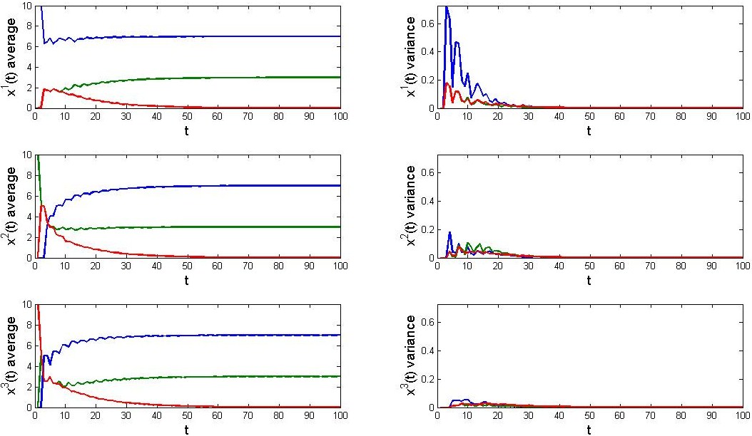
Figure 6: Plots of the sampled average (left) and variance (right) of players’ allocations $x^{i}(t)$, $i=1,2,3$ generated by bargaining protocol (18)–(20) for the robust game associated with the data in row I of Table 2. Sampled averages of the allocations $x^{i}(t)$ converge to the same point $\tilde{x}=[7\,3\,0]^{\prime}\in C(v^{\max})$, while sampled variances go rapidly to zero.

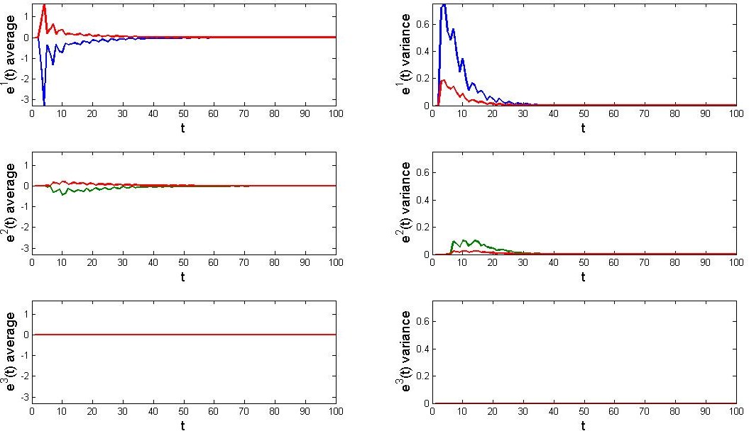
Figure 7: Plots of the sampled average (left) and sampled variance (right) of the errors $e^{i}(t)$, $i=1,2,3$ for the bargaining protocol (18)–(20) and the robust game associated with the data in row I of Table 2. Sampled averages and the variances of the errors $e^{i}(t)$ converge to zero.

In Figures 6 and 7, we report our simulation results for the average of the sample trajectories obtained by Monte Carlo runs. Figure 6 shows the sampled average and variance of the allocations $x^{i}(t)$, $i=1,2,3$ per iteration $t$. In accordance with the convergence result of Theorem 1, the sampled averages of the players’ allocations $x^{i}(t)$ converge to the same point, namely $x=[7\,3\,0]^{\prime}$ which is in the core of the robust game $C(v^{\rm max})$. Figure 7 shows that the sample average and sampled variance of the errors $e^{i}(t)$ converge to 0, as expected in view of Lemma 3(b).

5.1.2 Average game

In this numerical example, for scenario I data as given in row I of Table 2, we consider the average TU game and its corresponding bargaining protocol (32)–(34). We at first provide a sample example and report the outcomes for the first three steps of the algorithm, as reported below:

$$\begin{array}[]{l}\bar{v}(0)=[5.5\;1.6\ldots 10]^{\prime}\\ \bar{v}(1)=[4.8\;1.8\ldots 10]^{\prime}\\ \bar{v}(2)=[4.6\;1.8\ldots 10]^{\prime}\\ \bar{v}(3)=[4.7\;1.8\ldots 10]^{\prime}\end{array}\,\begin{array}[]{l}x^{1}(0)=[10\;0\;0]^{\prime}\\ x^{1}(1)=[10\;0\;0]^{\prime}\\ x^{1}(2)=[5\;2.5\;2.5]^{\prime}\\ x^{1}(3)=[4.7\;2.6\;2.7]^{\prime}\end{array}\,\begin{array}[]{l}x^{2}(0)=[0\;10\;0]^{\prime}\\ x^{2}(1)=[0\;5\;5]^{\prime}\\ x^{2}(2)=[0\;5\;5]^{\prime}\\ x^{2}(3)=[2.5\;3.75\;3.75]^{\prime}\end{array}\,\begin{array}[]{l}x^{3}(0)=[0\;0\;10]^{\prime}\\ x^{3}(1)=[0\;5\;5]^{\prime}\\ x^{3}(2)=[5\;2.5\;2.5]^{\prime}\\ x^{3}(3)=[5\;2.5\;2.5]^{\prime}.\end{array}$$

Recalling that the initial players’ allocations are $x^{1}(0)=[10\;0\;0]^{\prime}$, $x^{2}(0)=[0\;10\;0]^{\prime}$, and $x^{3}(0)=[0\;0\;10]^{\prime}$, we note that at time $t=1$, bargaining involves player 2 and 3 who update their allocations to $x^{2}(1)=[0\;5\;5]^{\prime}$ and $x^{3}(1)=[0\;5\;5]^{\prime}$, respectively. At time $t=2$, the bargaining involves player 1 and 3 who update their allocations, respectively, to $x^{1}(2)=[5\;2.5\;2.5]^{\prime}$ and $x^{3}(2)=[5\;2.5\;2.5]^{\prime}$. Notice that the obtained allocations for $t=1,2$ are feasible for the bounding sets and, therefore, no projection is performed. Finally, at time $t=3$, the bargaining involves player 1 and 2 who update their allocations to $x^{1}(3)=[4.7\;2.6\;2.7]^{\prime}$ and $x^{2}(3)=[2.5\;3.75\;3.75]^{\prime}$, respectively. Here $x^{1}(3)$ results from projecting onto the bounding set of player 1.

For the average game associated with the data in row I of Table 2, we have $v^{\rm mean}=[5.5\ 1.5\ 0\ 0\ 0\ 0\ 10]^{\prime}$ and the core $C(v^{\rm mean})$ given by

$$C(v^{\rm mean})=\{x\in\mathbb{R}^{3}:\,x_{1}\geq 5.5,\,x_{2}\geq 1.5,\,x_{3}\geq 0,\,x_{1}+x_{2}\geq 0,\,x_{1}+x_{3}\geq 0,$$

$$x_{2}+x_{3}\geq 0,\,x_{1}+x_{2}+x_{3}=10\}.$$

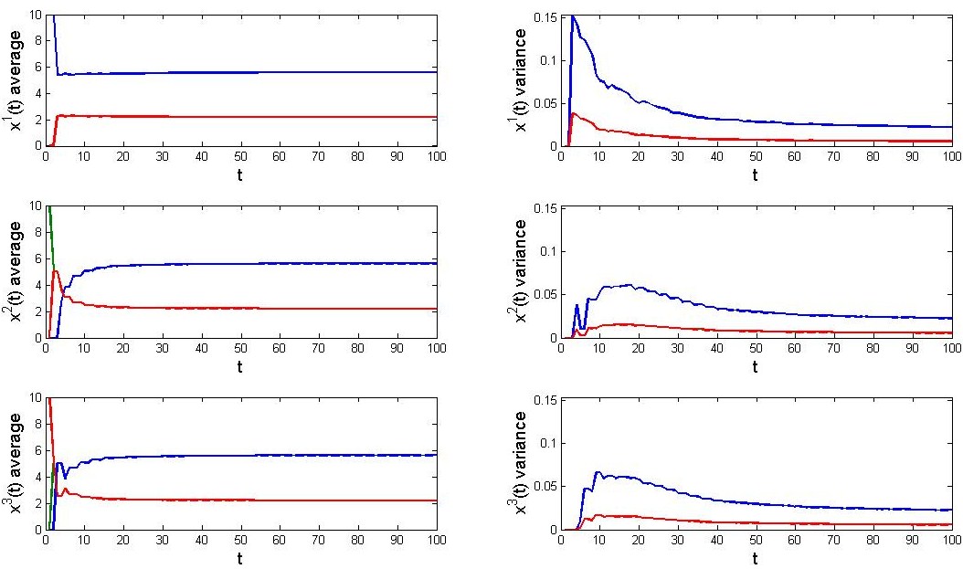
Figure 8: Plots of the sampled averages (left) and variances (right) of players’ allocations $x^{i}(t)$, $i=1,2,3,$ obtained by bargaining protocol (32)–(34) for the average game associated with the data in row I of Table 2. Sampled averages converge to point $\tilde{x}=[5.6\ 2.2\ 2.2]^{\prime}\in C(v^{\rm mean})$, which is the average of the limit points of the 50-sample trajectories.

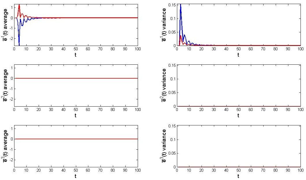
Figure 9: Plots of the sampled average (left) and variance (right) of the errors $\bar{e}^{i}(t)$, $i=1,2,3,$ for bargaining protocol (32)–(34) and the average game associated with the data in row I of Table 2. The sampled average and variance of the errors $\bar{e}^{i}(t)$ goes to 0.

In Figures 8 and 9, we depict our simulation results generated by bargaining protocol (32)–(34) for the average game. Figure 8 shows that the sampled average of the allocations $x^{i}(t)$, $i=1,2,3$ converge to a common point $\tilde{x}=[5.6\ 2.2\ 2.2]^{\prime}$ which belongs to the core $C(v^{\rm mean})$ of the average game, as guaranteed by Theorem 3. The sampled variance does not converge to zero as the common limit point of the allocations $x^{i}(t)$ can be different for different runs. Figure 9 demonstrates that the sampled average and variance of the errors $\bar{e}^{i}(t)$, $i=1,2,3,$ converge to zero, as predicted by Lemma 7(b).

5.2 Simulation Scenario II

Here, we report the simulation results obtained by the bargaining protocol (32)–(34) for the average game corresponding to the data in row II of Table 2. In this case the core of the robust game is empty, so we do not consider the robust game. The average game has characteristic function $v^{\rm mean}=[6.5\,2.5\,0\,0\,0\,0\,10]^{\prime}$ and its core is

$$C(v^{\rm mean})=\{x\in\mathbb{R}^{3}:\,x_{1}\geq 6.5,\,x_{2}\geq 2.5,\,x_{3}\geq 0,\,x_{1}+x_{2}\geq 0,\,x_{1}+x_{3}\geq 0,$$

$$x_{2}+x_{3}\geq 0,\,x_{1}+x_{2}+x_{3}=10\}.$$

Figures 10 and 11 show the results for the average game obtained in our simulations. In Figure 10, we report the sampled averages of the players’ allocations $x^{i}(t)$, $i=1,2,3$, obtained by bargaining protocol (32)–(34). In accordance with Theorem 3, the players’ allocations converge to an allocation that lies in the core of the average game $C(v^{\rm mean})$, precisely to the point $\tilde{x}=[6.6\ 2.6\ 0.8]^{\prime}\in C(v^{\rm mean})$. Here, again, the sampled variance of the allocations does not converge to zero as their common limit point is different for different runs. Figure 11 shows that the sampled average and variance of the errors $\bar{e}^{i}(t)$, $i=1,2,3$, converge to zero.

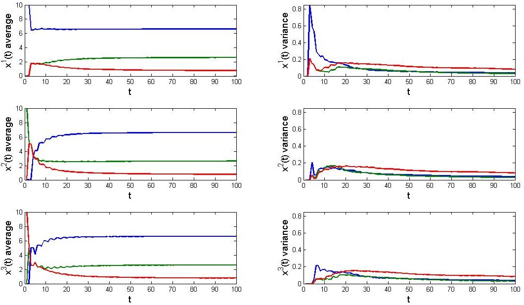
Figure 10: Plots of the sampled averages (left) and variances (right) of the players’ allocations $x^{i}(t)$, $i=1,2,3$ obtained by the bargaining protocol (32)–(34) for the average game associated with the data in row II of Table 2. Sampled averages converge to point $\tilde{x}=[6.6\ 2.6\ 0.8]^{\prime}\in C(v^{\rm mean})$, which is the average of the limit points of the 50-sample trajectories.

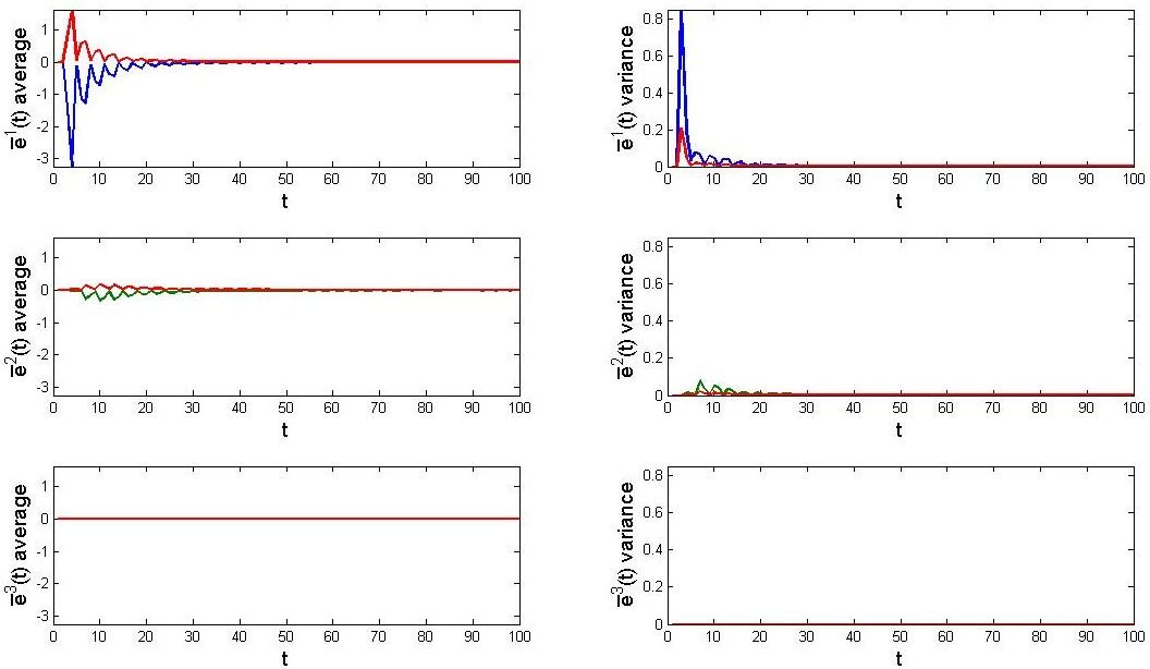
Figure 11: Plots of the sampled average and variance of the errors $\bar{e}^{i}(t)$, $i=1,2,3$ for the bargaining protocol (32)–(34) and the average game associated with the data in row II of Table 2. The sample average and variance of the errors $\bar{e}^{i}(t)$ converge to zero.

6 Conclusions

This article deals with dynamics and robustness within the framework of coalitional TU games. With respect to a sequence of TU games, each with a random characteristic function, the novelty of the work lies in the design of a decentralized allocation process defined over a communication graph of players. The allocation process captures the main features of bargaining in a realistic scenario. The proposed bargaining scheme is proven to converge, with probability 1, in either a robust game setting or an average game setting, under mild assumptions on the communication topology among the players and the stochastic properties of the random characteristic function. The key properties that distinguish this work from the existing work on dynamic games are: (1) the introduction of a time-varying communication graph, termed players’ neighbor-graph, over which the bargaining protocol takes place; and (2) the distributed bargaining protocol for players’ allocations updates subject to local information exchange with neighboring players.

References

- [1] T. Arnold and U. Schwalbe. Dynamic coalition formation and the core. Journal of Economic Behavior and Organization, 49:363–380, 2002.
- [2] D. Bauso, F. Blanchini, and R. Pesenti. Optimization of long-run average-flow cost in networks with time-varying unknown demand. IEEE Transactions on Automatic Control, 55(1):20–31, 2010.
- [3] D. Bauso and P. V. Reddy. Robust allocation rules in dynamical cooperative TU games. Proc. of the 49th Conference on Decision and Control, 2010.
- [4] D. Bauso and J. Timmer. Robust dynamic cooperative games. International Journal of Game Theory, 38(1):23–36, 2009.
- [5] J.C. Cesco. A convergent transfer scheme to the core of a TU-game. Revista de Matemáticas Aplicadas, 19(1–2):23–35, 1998.
- [6] J. Drechsel. Cooperative Lot Sizing Games in Supply Chains. Springer-Verlag. Series: Lecture Notes in Economics and Mathematical Systems, Berlin, Germany, 1 edition, 2010.
- [7] F. Facchinei and J-S. Pang. Finite-dimensional variational inequalities and complementarity problems, volume I-II. Springer-Verlag, New York, 2003.
- [8] J.A. Filar and L.A. Petrosjan. Dynamic cooperative games. International Game Theory Review, 2(1):47–65, 2000.
- [9] D. Granot. Cooperative games in stochastic characteristic function form. Management Sci., 23:621–630, 1977.
- [10] B.C. Hartman, M. Dror, and M. Shaked. Cores of inventory centralization games. Games and Economic Behavior, 31:26–49, 2000.
- [11] A. Haurie. On some properties of the characteristic function and the core of a multistage game of coalitions. IEEE Transactions on Automatic Control, 20(2):238–241, 1975.
- [12] A.J. Hoffman. On approximate solutions of systems of linear inequalities. Journal of Research of the National Bureau of Standards, 49:263–265, 1952.
- [13] E. Lehrer. Allocation processes in cooperative games. International Journal of Game Theory, 31:341–351, 2002.
- [14] A. Nedić, A. Olshevsky, A. Ozdaglar, and J.N. Tsitsiklis. Distributed subgradient methods and quantization effects. Proc. of the 47th CDC Conference, 54(11):4177–4184, 2008.
- [15] A. Nedić, A. Olshevsky, A. Ozdaglar, and J.N. Tsitsiklis. On distributed averaging algorithms and quantization effects. IEEE Transactions on Automatic Control, 54(11):2506–2517, 2009.
- [16] A. Nedić and A. Ozdaglar. Distributed subgradient methods for multi-agent optimization. IEEE Transactions on Automatic Control, 54(1):48–61, 2009.
- [17] A. Nedić, A. Ozdaglar, and P.A. Parrilo. Constrained consensus and optimization in multi-agent networks. IEEE Transactions on Automatic Control, 55(4):922–938, 2010.
- [18] B. T. Polyak. Introduction to Optimization. Optimization Software, Inc., New York, 1987.
- [19] S. Sundhar Ram, A. Nedić, and V.V. Veeravalli. Incremental stochastic subgradient algorithms for convex optimization. SIAM Journal on Optimization, 20(2):691–717, 2009.
- [20] S. Sundhar Ram, A. Nedić, and V.V. Veeravalli. Distributed stochastic subgradient algorithm for convex optimization. Journal of Optimization Theory and Applications, 147(3):516–545, 2010.
- [21] H. Robbins and D. Siegmund. A convergence theorem for nonnegative almost supermartingales and some applications. In Optimizing Methods in Statistics, pages 233–257. Academic Press, New York, 1971.
- [22] R. T. Rockafellar and R. J-B. Wets. Variational Analysis. Springer-Verlag, Berlin, Germany, 1998.
- [23] W. Saad, Z. Han, M. Debbah, A. Hjörungnes, and T. Başar. Coalitional game theory for communication networks. IEEE Signal Processing Magazine, Special Issue on Game Theory, 26(5):77–97, 2009.
- [24] J. Suijs and P. Borm. Stochastic cooperative games: Superadditivity, convexity, and certainty equivalents. Games and Economic Behavior, 27(2):331–345, 1999.
- [25] J. Timmer, P. Borm, and S. Tijs. On three shapley-like solutions for cooperative games with random payoffs. International Journal of Game Theory, 32:595–613, 2003.
- [26] J.N. Tsitsiklis. Problems in Decentralized Decision Making and Computation. PhD thesis, Dept. of Electrical Engineering and Computer Science, MIT, 1984.
- [27] J. von Neumann and O. Morgenstern. Theory of Games and Economic Behavior. Princeton Univ. Press, 1944.