Electron-nuclear dynamics in a quantum dot under non-unitary electron control

Abstract

We introduce a method for solving the problem of an externally controlled electron spin in a quantum dot interacting with host nuclei via the hyperfine interaction. Our method accounts for generalized (non-unitary) evolution effected by external controls and the environment, such as coherent lasers combined with spontaneous emission. As a concrete example, we develop the microscopic theory of the dynamics of nuclear-induced frequency focusing as first measured in Science 317, 1896 (2007); we find that the nuclear relaxation rates are several orders of magnitude faster than those quoted in that work.

The nuclear environment in III-V quantum dots has been recognized in recent years as the main source of decoherence for the electron spin and thus constitutes an important hurdle for quantum technologies with these systems. The microscopic dynamics of the closed electron-nuclear spin system have been investigated in important recent theoretical contributions wangluke ; coishschliemanndenghu . In these works wangluke , controls have been represented as ideal, unitary rotations of the electron spin, and the nuclear polarization along the external field is taken to be unaltered during the electron evolution. This no longer is the case in experiments involving controls that couple the system to an additional bath, which can exchange polarization with the system. Such experiments are relevant because incoherent interactions are needed to initialize and read out the system. These experiments in quantum dots (QDs) observed dynamic nuclear polarization and nuclear feedback effects greilichnuclei ; bracker ; sam . While the details of the various experiments differ, the main common feature is that an external control interacts with the electron, and through the hyperfine interaction the nuclear spins are also partially polarized. The theories employed to describe such experiments are usually in the form of rate equations and some sort of Fermi golden rule, and typically invoke phenomenological terms. Other theories christtaylor employed a more microscopic approach, but without including, e.g., feedback and a complete treatment of control fields.

In this Letter, we develop a theory that addresses such experiments involving non-unitary evolution of the electron while still treating the electron-nuclear interaction microscopically. We make use of the operator sum representation of quantum evolution and its simplified form in the spin vector (SV) representation and develop a theory that is perturbative with respect to the hyperfine coupling. We develop both Markovian and non-Markovian treatments, and by comparison of the two we establish the validity regime of the Markovian approximation.

In order to illustrate the power of our approach, we apply it to the experiment of Ref.greilichnuclei , a proper microscopic theory of which is lacking to date. This experiment demonstrated nuclear-induced focusing of the electron precession rates in a QD ensemble through the feedback dynamics of the electron and nuclear spins. This mechanism is largely driven by non-unitary evolution of the electron spin, making it difficult to solve conventional Master Equations to analyze the dynamics. Instead, a phenomenological treatment was introduced in the Supporting Online Material of greilichnuclei and further developed in sam . Our microscopic solution does not invoke phenomenological quantities and provides a unified description of the experiments in greilichnuclei ; sam . One of our striking results is that the nuclear relaxation process is several orders of magnitude faster than what is used in greilichnuclei ; sam .

The system we consider is a single electron trapped in a QD and subject to an external in-plane static magnetic field $B_{z}$, which splits the spin states along the $z$ direction. The electron interacts through the hyperfine contact interaction with $N$ nuclear spins in the QD ($N\approx 10^{5}$). There is also an external time dependent field acting on the electron, as well as the photon bath that drives spontaneous emission (electron-hole recombination). The total Hamiltonian is $H=H_{0}+H_{hf}+H_{p}+H_{rad}$, where

$$H_{0} = \omega_{e}\hat{S}_{z}+\epsilon_{T}|T\rangle\langle T|+\omega_{n}{\sum}_{i}\hat{I}^{i}_{z}$$ (1)

$$H_{hf} = {\sum}_{i}A_{i}\hat{S}_{z}\hat{I}^{i}_{z}+{\sum}_{i}{A_{i}}/{2}(\hat{S}_{+}\hat{I}^{i}_{-}+\hat{S}_{-}\hat{I}^{i}_{+})$$ (2)

$$H_{p} = \Omega(t)|\bar{x}\rangle\langle T|+h.c.$$ (3)

$$H_{rad} = {\sum}_{k}g_{k}(|z\rangle\langle T|+|\bar{z}\rangle\langle T|)a_{k}^{\dagger}e^{i\omega_{k}t}+h.c.$$ (4)

In Eqs. (1)-(4), $\hat{S}_{j}(\hat{I}_{j})$ is the electron (nuclear) spin operator along the $j$ axis, $\hat{S}_{\pm}=\hat{S}_{x}\pm i\hat{S}_{y}$, $\Omega(t)$ contains the pulse information, $|z\rangle(|\bar{z}\rangle)$ is the spin up (down) state along the B-field direction, $|\bar{x}\rangle$ is the spin down state along the optical axis $x$, $|T\rangle$ is the excited trion state, $g$ is the coupling to the radiation bath, and $a^{\dagger}$ is the bath photon creation operator. In the hyperfine Hamiltonian $H_{hf}$, the first term is referred to as the Overhauser term, while the second is called the ‘flip-flop’ term.

The couplings $\Omega(t)$ arise from periodic, ultrafast laser fields like those used in greilichnuclei . Since $A_{i}/\omega_{e}\ll 1$ for moderate magnetic fields, we give a perturbative treatment in this small parameter. We first focus on the zeroth order solution (electron spin periodically driven without nuclear coupling).

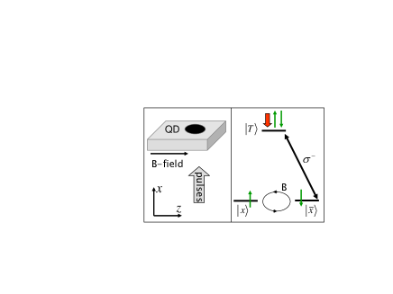
Figure 1: Color online. Left: Experimental setup of greilichnuclei ; sam . Right: Relevant QD states and polarization selection rules.

The primary effect of the pulses on the electron spin dynamics is the creation or destruction of spin polarization depending on the spin state. This arises from the selection rules of the three-level system in conjunction with the perpendicular external magnetic field. For concreteness, we consider $\sigma^{-}$ pulses, in which case only $|\bar{x}\rangle$ is coupled to the light and excited by it to the trion, see Fig. 1. Depending on the pulse parameters, a certain population is moved to the trion. This population subsequently decays back to the spin subspace via spontaneous emission of a photon. Due to the B-field, the population decays equally to the $|x\rangle$ and $|\bar{x}\rangle$ states, changing the electron spin polarization economou05 .

This physics describes non unitary evolution of the electron spin due to the coupling of the system to the photon bath. To describe this mathematically in the spin subspace we need a generalization of the usual unitary evolution operator to a set of so-called Kraus operators $\{E_{j}\}$ which transform the density matrix as $\sum_{j}E_{j}\rho E^{\dagger}_{j}$ nielsenchuang . These can be found by solving for the non-unitary part of the evolution of an arbitrary initial system density matrix and relating it to the final density matrix. Following this standard procedure supplement we find the following Kraus operators in the $|x\rangle,|\bar{x}\rangle$ basis

$$E_{1}=\left[\begin{array}[]{cc}1&0\\ 0&q\\ \end{array}\right],~{}E_{2}=\left[\begin{array}[]{cc}0&k\\ 0&0\\ \end{array}\right],~{}E_{3}=\left[\begin{array}[]{cc}0&0\\ 0&k\\ \end{array}\right],$$ (11)

where $q=q_{o}e^{i\phi}$ and $k=\sqrt{\frac{1-q_{o}^{2}}{2}}$. The parameter $q_{o}^{2}$ is the probability to go from $|\bar{x}\rangle$ to $|\bar{x}\rangle$; it is related to the pulse area and takes values from 0 to 1. The quantity $(1-q_{o}^{2})$ is related to the probability of population remaining in the trion state after the passage of the pulse, and thus $q_{o}$ quantifies the deviation from unitary dynamics in the qubit subspace (for unitary evolution $q_{o}=1$). The parameter $\phi$ is the spin rotation angle caused by the pulse and is a function of the detuning. We have therefore found 2-d matrices to describe the more complicated dynamics of the pulse followed by spontaneous emission.

In between pulses the evolution is simply Larmor precession under $B_{z}$, given by $U=e^{-i\omega_{e}T_{R}\hat{S}_{z}}$, where $T_{R}$ is the period of the pulse train. We are interested in finding the steady state electron spin. For this, the SV representation ($S_{e,j}=2\hbox{Tr}(\rho\hat{S}_{j})$) is most convenient as all the operations act on the left side of the SV. As a result of the non-unitarity of the evolution, in addition to the transformation of the SV a new contribution is generated at each cycle:

$$S_{e}(nT_{R})=S_{e}^{(n)}=Y_{e}S_{e}^{(n-1)}+K_{e},$$ (12)

where we found that $(Y_{e})_{ij}=2\sum_{\ell}\text{Tr}\left[\hat{S}_{i}E_{\ell}U\hat{S}_{j}U^{\dagger}E_{\ell}^{\dagger}\right],$ $(K_{e})_{j}=2\sum_{\ell}\text{Tr}\left[\hat{S}_{j}E_{\ell}E_{\ell}^{\dagger}\right]$. In the limit $n\rightarrow\infty$ the steady state is $S_{e}^{(\infty)}=(1-Y_{e})^{-1}K_{e}$ (explicit expression is in supplement ). We therefore see that a $3\times 3$ matrix, $Y_{e}$, and a three-dimensional vector, $K_{e}$, are the quantities that determine the dynamics of the electron spin. Because its structure is convenient we use the equivalent and more compact $4\times 4$ matrix that contains all the information:

$$\mathcal{Y}_{e}=\left[\begin{array}[]{cccc}1&0&0&0\\ K_{e,x}&Y_{e,xx}&Y_{e,xy}&Y_{e,xz}\\ K_{e,y}&Y_{e,yx}&Y_{e,yy}&Y_{e,yz}\\ K_{e,z}&Y_{e,zx}&Y_{e,zy}&Y_{e,zz}\end{array}\right].$$ (17)

In this 4-d representation, the steady-state SV $\mathcal{S}_{e}^{(\infty)}=(1,S_{e,x}^{(\infty)},S_{e,y}^{(\infty)},S_{e,z}^{(\infty)})$ is the eigenvector of $1-\mathcal{Y}_{e}$ with eigenvalue 0. This more compact representation will prove very useful when we introduce the nuclear spin.

Having solved the zeroth order problem, we proceed to the inclusion of the hyperfine interaction. For simplicity we assume that the nuclear spin has $I=1/2$. The nuclear spins affect each other through their interactions with the electron. When $A\sqrt{N}/\omega_{e}\ll 1$, where $A$ is a typical value of $A_{i}$, flip-flops occur slowly so that multinuclear effects such as dark state saturation christtaylor are negligible, and the primary effect of the nuclear spins on the electron is a shift of the precession frequency through the Overhauser term (Overhauser shift). Therefore, we consider first a single nuclear spin interacting with the electron and incorporate multinuclear effects by shifting the electron Zeeman frequency by an amount proportional to the net nuclear polarization greilichnuclei ; sam .

For a single nuclear spin interacting with the electron spin via the hyperfine Hamiltonian we use a SV representation, which in this case is 15-d. For the type of control used in Ref. greilichnuclei ; sam , there are no nuclear effects during the ultrashort (i.e., broadband) pulses, which do not distinguish between the electron spin eigenstates along the field $B_{z}$. Therefore, the Kraus operators are simply tensor products between the $E_{j}$’s of Eq. (11) and the identity. Following the same prescription as for the single spin, we define a 16-d SV $\mathcal{S}_{i}=4\text{Tr}\left(\rho G_{i}\right),$ where $\rho$ is the $4\times 4$ density matrix of the two spins and the generators $G_{i}$ are tensor products of spin operators (including the identity) $G_{4k+\ell}=\hat{S}_{k}\otimes\hat{I}_{\ell}$, where $k,\ell$ run from 0 to 3. With our conventions, $\mathcal{S}_{0}=1$. The 16-d analogue of $\mathcal{Y}_{e}$ is given by $\mathcal{Y}_{ij}=4\sum_{\ell}\text{Tr}\left[G_{i}E_{\ell}U_{e,n}G_{j}U_{e,n}^{\dagger}E_{\ell}^{\dagger}\right]$. In general $\mathcal{S}$ is not simply a tensor product of the two individual SVs, but contains quantum correlations (entanglement).

The pulses are expected to ‘interrupt’ the electron-nuclear evolution only for $q_{o}\ll 1$, while entanglement will build up when $q_{o}\sim 1$. Therefore a Markovian approximation should be sufficient for short pulse train periods and pulses of strength $q_{o}\sim 0$ (as in greilichnuclei ; sam ) .

Markovian approximation–To find an effective relaxation rate for the nuclear spin, we use the equation $\mathcal{S}(t+T_{R})=\mathcal{Y}\mathcal{S}(t)$ for the 16-d case. In the Markovian approximation, we only keep the separable (tensor product) part of $\mathcal{S}$, i.e., $\mathcal{S}=\mathcal{S}^{(\infty)}_{e}\otimes\mathcal{S}_{n}$, where we have used that the timescales of evolution for the electron and the nuclei are quite different merkulov , so that we can assume that the electron steady state is reached quickly compared to the nuclear dynamics greilichnuclei ; sam ; nazarov ; rudnerlevitov . The equation for the 4-d nuclear SV is then $\mathcal{S}_{n}(t+T_{R})=\mathcal{Y}_{n}\mathcal{S}_{n}(t),$ where $\mathcal{Y}_{n}$ explicitly contains electron SV components. Since the nuclear evolution is much slower than the pulse repetition rate, we can coarse grain this equation, and obtain a differential equation for the nuclear SV, $\frac{d}{dt}\mathcal{S}_{n}={1\over T_{R}}(\mathcal{Y}_{n}-1)\mathcal{S}_{n},$ which gives $\mathcal{S}_{n}(t)=e^{(\mathcal{Y}_{n}-1)t/T_{R}}\mathcal{S}_{n}(0).$ For small flip-flop coupling (but keeping the Overhauser term to all orders), we find the two smallest eigenvalues of $1-\mathcal{Y}_{n}$ to be $\lambda_{1}=0$ and

$$\lambda_{2}=\frac{A^{2}}{\omega_{e}^{2}}\frac{1+S_{e,z}^{2}+(S_{e}^{2}-1)\cos(\frac{AT_{R}}{2})}{1+S_{e,z}^{2}+(S_{e,z}^{2}-1)\cos(\frac{AT_{R}}{2})}\sin^{2}\frac{\omega_{e}T_{R}}{2},$$ (18)

where $S_{e}$ is the length of the electron steady state SV, and for brevity we have suppressed the superscript $\infty$ foot1b . The zero eigenvalue corresponds to the nuclear steady-state SV, which to leading order in the flip-flop term is $\mathcal{S}_{n}^{(\infty)}=(1,0,0,S_{n,z}^{(\infty)})$ where

$$S_{n,z}^{(\infty)}=\frac{2S_{e,z}[\sin^{2}\left(\frac{AT_{R}}{4}\right)+S_{e}^{2}\cos^{2}\left(\frac{AT_{R}}{4}\right)]}{1+S_{e,z}^{2}+(S_{e}^{2}-1)\cos(\frac{AT_{R}}{2})}.$$ (19)

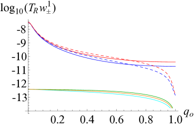
Figure 2: Color online. Plot of the log of the nuclear relaxation rates multiplied by $T_{R}$ from our current theory (upper set of curves) with our Markovian approximation (solid) and exact numerical (dashed) as function of $q_{o}$. The lower curves are based on Refs. greilichnuclei ; sam and are several orders of magnitude less. Pulse parameters are $\phi=\pi/2,T_{R}=3900.3/\omega_{e},A/\omega_{e}=10^{-5}.$

The nonzero eigenvalue $\lambda_{2}$ gives the nuclear relaxation rate $\gamma_{n}=\lambda_{2}/T_{R}$. The single nucleus spin flip rates, which are generally different in the presence of nonzero polarization sam , are $w^{1}_{\pm}=\gamma_{n}(1\pm S_{n,z}^{(\infty)})/2$, where $w^{1}_{+}$ ($w^{1}_{-}$) is the rate to flip from down (up) to up (down). Fig. 2 shows that our rates are orders of magnitude larger than those of greilichnuclei ; sam . The heuristic expressions only took into account that the relaxation rates should vanish when $T_{R}$ is a multiple of the electron spin precession period as well as the overall scale factor $A^{2}/\omega_{e}^{2}$. The first of these features arises because an electron spin synchronized with the pulses is unaffected by them so that no nuclear relaxation takes place. The scale factor is fixed by noting that energy conservation leads to a suppression of hyperfine flip-flops when $\omega_{e}\gg\omega_{n}$; only virtual flip-flops are allowed and since these must come in pairs, their effect is second-order in $A/\omega_{e}$.

Our theory reveals an additional dependence of the relaxation rate $\gamma_{n}$ on the orientation of the electron spin that was overlooked by greilichnuclei ; sam . When the electron SV is transverse to the B-field ($S_{e,z}\approx 0$ and $S_{e}\gg 0$), flip-flops are not suppressed by energy conservation and angular momentum is freely transferred from the electron to the nuclei, leading to a strong enhancement of $\gamma_{n}$. This is also clear from Eq. (18) where the denominator is close to zero when $S_{e,z}\approx 0$ while the numerator remains finite due to $S_{e}\gg 0$. These conditions are realized in the regime most relevant for the experiments in Refs. greilichnuclei ; sam where $q_{o}\ll 1$, that is, when the pulses drive most of the population out of the qubit subspace, re-orienting the electron spin along the optical ($x$) axis. Note that the enhancement of $\gamma_{n}$ depends crucially on the openness of the system since the photon bath acts as an angular momentum reservoir. Our predicted timescale can be checked experimentally by measuring in a single QD the frequency of the pump-probe signal at various timescales. By systematically varying the B-field and pulse parameters the relaxation rates could be mapped out as a function of the parameters.

The probability distribution for the net multinuclear polarization $m/2$ is obtained from a kinetic equation for $m$, which is the difference in the number of spins pointing up and down:

$$\frac{dP(m)}{dt} = -\sum_{\pm}\left[w_{\pm}(m){N\mp m\over 2}\right]P(m)$$

$$+ \sum_{\pm}P(m\pm 2)w_{\mp}(m\pm 2)\left[{N\pm m\over 2}+1\right],$$

where $w_{\pm}(m)$ are the rates in the presence of nuclear polarization $m/2$. These are found by implementing the Overhauser shift, $w_{\pm}(m)=w_{\pm}^{1}(\omega_{e}+mA)$, where we have assumed equal couplings for all nuclear spins foot3 . Examples of the resulting distribution are shown in Fig. 3 for typical values of the parameters. In general, large $T_{R}$ results in more peaks in $P(m)$ and thus gives rise to a greater degree of nuclear state “narrowing” ($T_{2}^{*}$ is enhanced). Furthermore, the sharpest peaks occur at values of $m$ such that $(\omega_{e}+mA)T_{R}$ is an odd integer multiple of $\pi$, and the locations of these peaks can be controlled by adjusting $\omega_{e}T_{R}$. A systematic exploration of the parameter space can help tailor the nuclear state.

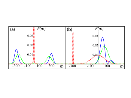
Figure 3: Color online. The nuclear polarization probability distribution with $N=5000$ nuclei and pulse parameters $\phi=\pi/4,q_{o}=0.2,A/\omega_{e}=10^{-5}$ and for (a) $T_{R}=797.9/\omega_{e}$ and (b) $T_{R}=800.3/\omega_{e}$, from our Markovian theory (blue/solid line), the theory from Ref.greilichnuclei (red/dotted) and the one from Ref.sam (green/dashed).

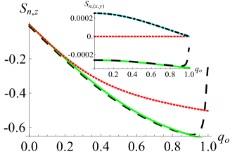
Figure 4: Color online. Nuclear steady state SV $z$ component as function of $q_{o}$ for Markovian approximation Eq. (19) (red/dotted), analytical non-Markovian, Eq. (21) (green/solid) and exact numerical (black/dashed) for $\phi=\pi/2,T_{R}=3900.3/\omega_{e},A/\omega_{e}=10^{-5}$. Inset shows $S_{n,x}$, $S_{n,y}$.

Beyond the Markovian approximation–Our analysis above provides analytic expressions for the nuclear dynamics in the Markovian approximation, an approach valid for $q_{o}\ll 1$ (see Fig. 2). Our formalism however is not inherently Markovian, and we now present an analytical non-Markovian expression for the nuclear steady state. We return to the 16-d matrix $\mathcal{Y}$ and perform a perturbative expansion in the coupling which is a controlled approximation in the hyperfine coupling. The steady state nuclear SV turns out to be

$$S_{n}^{(\infty)}=c(1+q_{o}^{2}-2q_{o}\cos\phi,(1-q_{o}^{2})\tan(\omega_{e}T_{R}/2),$$

$$\qquad\qquad q_{o}\omega_{e}T_{R}\sin\phi),$$ (21)

where $c$ is in foot2 . Nonzero $x,y$ components arise from expanding the Overhauser interaction in addition to the flip-flop in deriving Eqn. (21). Fig. 4 shows that the dynamics become less Markovian as the pulses become more unitary ($q_{o}\rightarrow 1$).

In conclusion, we have developed a formalism for analyzing experiments with generalized, non-unitary controls on the electron spin confined in a QD and coupled to the host nuclei. By applying it to the experiments of greilichnuclei ; sam we have found that the nuclear relaxation is orders of magnitude faster than previously thought. Our method is in general non-Markovian and is applicable to controls other than ultrafast lasers by appropriate choice of the Kraus operators. It can have wide application to other systems, such as gated QDs and NV centers in diamond dutt_nv . An interesting application of the theory would be to use it for the design of the final nuclear state.

This work was supported by LPS/NSA (EB) and in part by ONR and LPS/NSA (SEE).

References

- (1) W. Yao, R.-B. Liu, and L. J. Sham, Phys. Rev. B 74, 195301 (2006); L. Cywinski, W. M. Witzel and S. Das Sarma, Phys. Rev. B 79, 245314 (2009).
- (2) W. A. Coish, J. Fischer and D. Loss, Phys. Rev. B 81, 165315 (2010); B. Erbe and J. Schliemann, Phys. Rev. Lett. 105, 177602 (2010); C Deng and X. Hu, Phys. Rev. B 73 241303(R) (2006).
- (3) A. Greilich et al., Science 317, 1896 (2007).
- (4) A. S. Bracker et al., Phys. Rev. Lett. 94, 047402 (2005); D. J. Reilly et al., Science 321, 817 (2008); X. Xu et al., Nature 459, 1105 (2009); Foletti et al., Nature Phys. 5, 903 (2009); C. Latta et al., Nature Phys. 5, 758 (2009); T. D. Ladd et al., Phys. Rev. Lett. 105, 107401 (2010); E. A. Chekhovich et al., Phys. Rev. Lett. 104, 066804 (2010).
- (5) S. G. Carter et al., Phys. Rev. Lett. 102, 167403 (2009).
- (6) H. Christ et al., Phys. Rev. B 75, 155324 (2007); J. Taylor et al., Phys. Rev. Lett. 91, 246802 (2003).
- (7) S. E. Economou et al., Phys. Rev. B 71, 195327 (2005).
- (8) M. A. Nielsen and I. L. Chuang, Quantum Computation and Quantum Information (Cambridge Univ. Press).
- (9) See supplement.
- (10) I. A. Merkulov, Al. L. Efros, and M. Rosen, Phys. Rev. B 65, 205309 (2002).
- (11) J. Danon and Yu. V. Nazarov, arXiv:1011.3378 (2010).
- (12) M. S. Rudner and L. S. Levitov, Phys. Rev. Lett. 99, 246602 (2007).
- (13) We drop the nuclear Zeeman splitting, since .
- (14) The case of unequal hyperfine couplings can be treated by introducing a probability distribution and flip rates for each different value of the coupling and solving a set of rate equations like Eq. (Electron-nuclear dynamics in a quantum dot under non-unitary electron control).
- (15) , where is in supplement .
- (16) M. V. G. Dutt et al., Science 316, 1312 (2007).