On the dynamics of bubbles in boiling water

Abstract

We investigate the dynamics of many interacting bubbles in boiling water by using a laser scattering experiment. Specifically, we analyze the temporal variations of a laser intensity signal which passed through a sample of boiling water. Our empirical results indicate that the return interval distribution of the laser signal does not follow an exponential distribution; contrariwise, a heavy-tailed distribution has been found. Additionally, we compare the experimental results with those obtained from a minimalist phenomenological model, finding a good agreement.

1 Introduction

Bubbles are ubiquitous in nature and their dynamics is both fascinating and very complex[1, 2]. It is not surprising that bubbles are an effervescent source of research. For instance, bubbles appear in the context of energy generation[3, 4], collapsing bubbles can emit ligth[5], turbulent thermal convection has been observed in a single soap bubble[6], cooperative and avalanches-like dynamics are present in collapsing of aqueous foams[7, 8], and singularities emerge when air bubbles detache from a nozzle submerged in water[9].

Despite the fact that the fundamental equations ruling the behavior of moving fluids are well known, an analytical or even a numerical approach can become infeasible for many common situations. This is particularly true for bubbles in turbulent fluids, where, at higher Reynolds numbers, the number of mesh points required to solve each bubble as well as the flow around it grows up leading to a long simulation time[10].

A very familiar case, where bubbles appears in such contexts, is the boiling process of water[11]. For exemple, when the temperature reaches 100^∘C the vapor pressure is 1 bar and we can observe the spontaneous process of bubble formation (nucleation)[12]. Although it is an ordinary process, nucleate boiling has several complex aspects involving thermal interactions between bubbles and the heated surface and among the nucleation sites. There are also hydrodynamics interactions bubble to bubble and bubble to liquid bulk[13]. In this scenario, simple models, whether phenomenological or not, and simple experiments have been designed to try to clarify this intricate dynamics. For instance, extensive studies have been done by considering nonlinear models and experiments of boiling[13] as well as evaporation in microchannels[14] or in short capillary tube[15]. However, as far the authors know, much less attention has been paid to clouds of bubbles, i.e., a system containing many interacting bubbles (see for instance Ref.[16]). Our main goal here is attempt to fill this hiatus by using a simple experiment that basically consists of a laser beam passing through a sample of boiling water. We also comfront the experimental results with a minimalist model towards improving our understanding of this complex system.

This article is organized as follows. Primarily, we describe the experimental setup and the data acquisition. Next, we report a statistical analysis of the data and present a model. Finally, we end this work with some concluding comments and a summary.

2 Experimental setup and data presentation

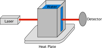
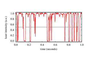
Figure 1: (left panel) A schematic representation of the experimental setup: a laser beam passes through a sample of boiling water which is in contact with the heat plate. The laser intensity is monitored by the detector (photodiode) and recorded. (right panel) A typical laser intensity signal for a sample of approximately 300 ml of boiling water.

The experiment consists of samples of approximately 300 ml of distilled water at atmospheric pressure and confined by impermeable metallic walls with glass windows through which the laser beam is transmitted, as shown in Figure 1 (left panel). At the bottom, the confining vessel is in contact with a heat plate that employs a power of around 300 W, in such way that the temperature in the contact interface is approximately 300 ^∘C. After the boiling process becomes stable, i.e., the water temperature stabilizes, we start to record the He-Ne laser (10 mW) intensity signal that passes through the sample by using a photodiode detector (Thorlabs DET100A) coupled to an oscilloscope (Tektronix TDS5032B) with a sampling rate of a thousand points per second. Typical recording times are of the order of 10 minutes and the height of the incident beam does not significantly change the statistical results, avoiding the water-air interface.

Figure 1 (right panel) shows a typical record signal. We can see that the signal is characterized by intermittent valleys. While the emerging dynamic is complex, the individual processes generating the bubble are qualitatively simple. At the button of the confining vessel the temperature is higher what makes a small fraction of the liquid to evaporate, producing the bubbles. These nucleation sites are not static and depend on the heat transfer and also on the liquid-wall interactions. The bubbles depart from the nucleation sites and rise through the confining vessel. Along this movement the bubbles continuously interact with each other, with the liquid and with the walls. When one or more bubbles crossing the laser path they scatter the light, producing a decrease in the record signal. Naturally, this intrincated signal reflects the complex collective dynamical behavior of the bubbles. Similar situations are customary when dealing with time series. For instance, the earth seismic and geomagnetic activity can be investigated by considering a seismogram and the DST index.

3 Data analysis

Due the conditions of the signal, a natural variable to investigate the system dynamics is the time difference between the extreme events characterized by sharped valleys. This analysis is frequently employed in the physics and financial literature[17, 18, 19, 20] and it shows to be useful when investigating the underling mechanism ruling the system[21, 22, 23, 24].

A possible manner to obtain these extreme events is considering a threshold value $q$ and archiving the initial times $t_{i}$ for which laser signal is below this edge. The difference between two consecutive times, $\tau_{i}=t_{i+1}-t_{i}$, is the so called return interval. This procedure is presented in Figure 1, where the right panel shows horizontal line segments representing the return intervals for $q=0.5$. Figure 2a displays the probability density functions (pdf) of $\tau_{i}$, $\rho(\tau)$, for three values of $q$.

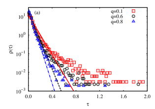
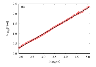
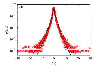
Figure 2: (a) Probability distribution of the return interval $\tau$ for three values of $q$ (indicated in the figure) in comparison with the exponential distribution of Eq.1 for $\bar{\tau}_{0.1}=0.0808$ (continuos line), $\bar{\tau}_{0.6}=0.0564$ (dashed line) and $\bar{\tau}_{0.8}=0.0438$ (dashed-dotted line). (b) DFA analysis for the laser intensity signal: $\log_{10}[F(n)]$ versus $\log_{10}(n)$ in comparison with a linear fit, where we found $F(n)\propto n^{h}$ with $h\approx 0.65$. (c) Distribution of scaled variable $\xi=\tau/\bar{\tau}_{q}$ for eight equally spaced threshold values from 0.1 to 0.9 in comparison with a stretched exponential (continuos line) and with a Weilbull distribution (dashed line) both with $\gamma=2(1-h)=0.7$. (d) Distribution of the return interval increments $\Delta\xi=\xi_{i+1}-\xi_{i}$ compared with Eq.3 when considering the stretched exponential (continuos line) and the Weilbull distribution (dashed line) both with $\gamma=0.7$. Notice that in the tail of the distributions the noise increases. This occurs because of the finite size of the set $\{\tau_{i}\}$ and also due to the small probability of finding large time intervals.

Clearly, the distribution is dependent on $q$, and it is also well known that for Gaussian random uncorrelated variables the return interval $\tau_{i}$ is exponentially distributed according to[25]

$$\rho(\tau)=\frac{1}{\bar{\tau}_{q}}e^{-{\tau}/{\bar{\tau}_{q}}}\,,$$ (1)

where $\bar{\tau}_{q}$ is the mean value of return interval related to the threshold value $q$. Figure 2a shows our data compared with this pdf, resulting in a poor agreement.

The weak agreement indicate that memory effects can be present in the bubble dynamics. To address this question, we may use the detrended fluctuation analysis (DFA)[26]. It basically consists of calculating the root mean square fluctuation function $F(n)$ (see for instance [27]) for the integrated and detrended time series for different values of the time scale $n$. When we have scale-invariant time series, $F(n)$ follows a power law behavior $F(n)\sim n^{h}$, where $h$ measures the degree of correlation in the time series: if $h=0.5$, the series is uncorrelated, while $h>0.5$ indicates long-range correlations. Figure 2b presents the results concerning the laser signal where we found $h\approx 0.65$ leading to long-range correlations.

Empirical results have claimed that in the presence of power law correlation in the data the pdf $\rho(\tau)$ is usually adjusted by a stretched exponential[21, 22, 23] or by a Weilbull distribution[24], i.e.,

$$\rho(\tau)\sim e^{-A\left({\tau}/{\bar{\tau}_{q}}\right)^{\gamma}}~{}~{}\text{or}~{}~{}\rho(\tau)\sim\left({\tau}/{\bar{\tau}_{q}}\right)^{\gamma-1}e^{-B\left({\tau}/{\bar{\tau}_{q}}\right)^{\gamma}}\,,$$ (2)

where $A$ and $B$ are constants and $\gamma$ is the exponent of the power law autocorrelation function. These two distributions also emerge in the analytical approach of Santhanam and Kantz[25] when considering a Gaussian fractional noise with autocorrelation exponent $\gamma$. It is interesting to note that by employing the scaled variable $\xi=\tau/\bar{\tau}_{q}$ both distributions become independent on $q$ and that the exponents $\gamma$ and $h$ are related via $\gamma=2(1-h)$. Figure 2c displays the distributions of the scaled variable $\xi$ and also the stretched exponential and the Weilbull distributions, which, due to the normalization and the unitary mean value of $\xi$, have just one parameter, $\gamma$, determined from $h$. From this figure, we observe a good data collapse but a poor agreement with both previous distributions, specially for small $\xi$. In this case, the distributions of Eq.2 underestimate the data for $\xi\in[0,2]$ and overestimate for $\xi\in[3,7]$. The agreement is not improved if we find $\gamma$ via least square method.

Another aspect to be investigated is the scaled return interval increments $\Delta\xi=\xi_{i+1}-\xi_{i}$. We know that the pdf of the difference between two independent random numbers $X-Y$ is given by the cross-correlation[28]

$$f_{X-Y}(\tau)=\int_{-\infty}^{\infty}f_{X}(x)f_{Y}(x+\tau)dx\,,$$ (3)

where $X$ is distributed according to $f_{X}(x)$ and $Y$ according to $f_{Y}(x)$. In the case of $\Delta\xi$, both distributions are the same and we can use a stretched exponential or the Weibull of Eq.2 to compare with the data. Figure 2d shows this comparison, again finding an imperfect agreement. In addition, we have to mention that the return interval series is week correlated ($h\approx 0.55$), thus the previous equation should be viewed as an approximation.

4 Modeling

In principle, we should be able to describe the dynamics of boiling fluid since the physical transport phenomena are well known to follow the Navier-Stokes equation. However, technical difficulties as numerical instability because of the complex boundary of the two phases and the large amount of simulation time required to do the integrations make this task very difficult. Thus, our goal is to understand this complex phenomenon from a minimalist model. Therefore, we retain only the relevant ingredients to reproduce the main aspects of the experimental data.

In an approximate scenery, we can employ a two-state model for which only matters whether there are bubbles in the laser path or not. When there are bubbles, the laser bean is considered totally scattered and the passing intensity signal is zero. On the other hand, when there are no bubbles, the beam passes without scattering and the intensity signal is one.

In addition to the above two-state approximation for the laser signal, a significant ingredient of these empirical data is the power law correlation presented in Figure 2b. It has been reported that a symbol series (here 0 or 1) can present long-range correlations when it is generated by using only two uncorrelated random numbers[29, 30]. In this context, a possible way to model our data is considering a one-dimensional lattice where the sites represent the laser intensity signal in a given time. In the first site of the lattice we start to fill it drawing a discrete random number from a Bernoulli distribution with probability parameter $p$. If the random number is 1, there are bubbles in the laser patch and the laser signal is zero for this time. Otherwise, there are no bubbles in the laser path and the laser signal is one for this time and also for the next $[x]$ times (sites), where $[x]$ is the integer part of a random number $x$ distributed according to a distribution $P(x)$. All of the other sites of this lattice are filled by repeating the above procedure. Due to the fact that the simulated laser signal is only zeros or ones, it does not depend on the threshold value $q$. Actually, in this approach the return interval $\tau$ is exactly the length of the consecutive zero sites. Thus, we effectively focus our attention on the the scaled variable $\xi$.

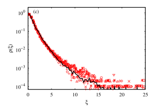
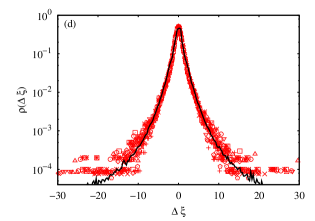
Figure 3: A comparison between the experimental (a) and the simulated (b) return intervals. The simulated result was obtained by considering a Pareto distribution with $k=1$ and $\alpha=1.8$ and the parameter $p=0.2$ for a lattice with $5\times 10^{4}$ sites averaged over $200$ realizations. Figure (c) shows the distribution of the return interval for eight equally spaced threshold values from 0.1 to 0.9 compared with the simulated result (continuos lines). Figure (d) presents the comparison for the return interval increments $\Delta\xi=\xi_{i+1}-\xi_{i}$.

The proposed model appears to be very ad hoc since we have a function to choose plus a parameter. However, when performing the simulations, we empirically found that short tail distributions such as exponential, Gaussian, lognormal, and gamma are not able to improve the agreement found when comparing with the analytical expressions of Eq.2. In contrast, when considering the most simple distribution with power law tail, i.e., the Pareto one

$$P(x)=\begin{cases}\alpha k^{\alpha}x^{-\alpha-1}&\text{if $x>k$,}\\ 0&\text{if $x<k$,}\end{cases}$$ (4)

where $k>0$, $\alpha>0$ are parameters of the distribution, the agreement with our data is very good.

Figure 3 shows the simulated return interval in comparison with experimental data. For the simulation, we have fixed the value $k=1$ and the size of lattice in a such way to have $5\times 10^{4}$ return intervals, typically the number found in the experimental data. To obtain the best fit parameters, we incrementally update the values of $\alpha$ and $p$ getting the distribution $\rho(\xi)$ which is averaged over $200$ realizations and so confronted with the experimental data via the method of least squares. The best values found for these parameters are $\alpha=1.8$ and $p=0.2$.

The previous model claims for an analytical approach. Indeed, it may be view as a sum of random numbers in which the number terms is also a random number. Thus, supposing known the distribution of Pareto sums, we may write

$$\rho(\tau)=N\sum_{n=1}^{\infty}(1-p)^{n}S_{n}(\alpha_{n},k_{n})\,,$$ (5)

where $N$ is the normalization factor, $(1-p)^{n}$ is the probability of summing $n$ consecutive numbers and $S_{n}(\alpha_{n},k_{n})$ is the distribution of Pareto sums. However, to obtain a general expression for $S_{n}(\alpha_{n},k_{n})$ may not be a easy task[31, 32, 33]. It can be argued that these cumbersome calculations are avoided if we consider a stable distribution for $P(x)$. In fact, for this case the sum of stable variables is well known to be a stable distribution, but the support of $P(x)$ is only positive when the stable index, $\alpha^{\prime}$, is less that one and the skewness parameter is equals to one[34]. The stable distribution is asymptotically a power law with $P(x)\sim x^{-1-\alpha^{\prime}}$ which is not compatible the exponent found when considering the Pareto distribution.

The comparison with the previous model also indicates that the laser signal is very close to a point possess, since the deflection times are very short when compared with inter-event times $\tau_{i}$. By comparing our model with Refs.[35, 36, 37], we find that the laser signal can be viewed as non-Poisson renewal process. This process is characterized by a sequence of events spaced by time intervals that are independent random variables. Moreover, the time intervals are draw from the same probability density $\psi(\tau)\sim\tau^{-\mu}$, where $\mu$ is the renew index. Confronting this expression with the Pareto distribution, we can see that the renew index is $\mu=\alpha+1\approx 2.8$ for our case. In addition, following Grigolini et. al[35], it is also possible to show that a fully asymmetric Lévy stable distribution of index $\delta=(\mu-1)^{-1}\approx 0.56$ emerges for number of events in an time interval $\tau^{\prime}$. Further, the renew process may be also connected with a noise whose power spectrum is $1/f^{\eta}$, where $\eta=3-\mu\approx 0.2$ in our case.

The previous findings suggest that a $1/f^{0.2}$ noise is present in the context of a first-order phase transition, in contrast with the common association among inverse power laws noise and critical phenomena[38, 39]. This has been also reported in the context of first-order electronic phase transitions[40] and for polymer folding[41]. From a general point of view, all the empirical discoveries suggest that, at boiling temperature, the fluctuations between the two phases (here, the bubble and the liquid bulk) play an essential role in the system dynamics, generating the nontrivial aspects reported here.

5 Summary

We have reported statistical analysis from the bubbles dynamics in a sample of boiling water. Our analysis was focused on an experiment of laser scattering in which a laser beam passed through the boiling fluid having its intensity monitored. By using this time series we evaluated the return interval distribution finding a non-exponential distribution. In addition, we verified that the dynamical processes that generates the bubbles introduces nontrivial correlations. Employing a minimalist phenomenological model we were able to reproduce the experimental behavior successfully . The model also seems to suggest that a fundamental ingredient generating the nontrivial dynamics is the power law tail related to the waiting time for the bubbles passing through the laser path and also the correlations introduced by the draw of the two random numbers.

References

- [1] Prosperetti A. Bubbles. Phys. Fluids 2004;16:1852-1865.
- [2] Lohse D. Bubble puzzles. Physics Today 2003;56:36-41.
- [3] Joshi JB. Computational flow modelling and design of bubble column reactors. Chem. Eng. Sci. 2001;56:5893-5933.
- [4] Alvarez-Ramirez J, Espinosa-Paredes G, Vazquez A. Detrended fluctuation analysis of the neutronic power from a nuclear reactor. Physica A 2005;351:227-240
- [5] Brenner MP, Hilgenfeldt S, Lohse D. Single-bubble sonoluminescence. 2002;74:425-484.
- [6] Seychelles F, Amarouchene Y, Bessafi M, Kellay H. Thermal convection and emergence of isolated vortices in soap bubbles. Phys. Rev. Lett. 2008;100. 144501,1-4
- [7] Vandewalle N, Lentz JF, Dorbolo S, Brisbois F. Avalanches of popping bubbles in collapsing foams. Phys. Rev. Lett. 2001;86:179-182.
- [8] Ritacco H, Kiefer F, Langevin D. Lifetime of bubble rafts: Cooperativity and avalanches. Phys. Rev. Lett. 2007;98. 244501,1-4.
- [9] Schmidt LE, Keim NC, Zhand WW, Nagel SR. Memory-encoding vibrations in a disconnecting air bubble. Nature Phys. 2009;5:343-346.
- [10] Tryggvason G, Esmaeeli A, Lu J, Biswas S. Direct numerical simulations of gas/liquid multiphase flows. Fluid Dynam. Res. 2006;38:660-681.
- [11] Zahn D. How does water boil? Phys. Rev. Lett. 2004;93. 227801,1-4.
- [12] Brennen CE. Cavitation and Bubble Dynamics. New York: Oxford University Press; 1995.
- [13] Shoji M. Studies of boiling chaos: a review. Int. J. Heat Mass Transfer 2004;47:1105-1128.
- [14] Thome JR. Boiling in microchannels: a review of experiment and theory. Int. J. Heat Fluid Flow 2004;25:128-139.
- [15] Cordonet A, Lima R, Ramos E. Two models for the dynamics of boiling in a short capillary tube. Chaos 2001;11:344-350.
- [16] Iida Y, Lee J, Kozuka T, Yasui K, Towata A, Tuziuti T. Optical cavitation probe using light scattering from bubble clouds. Ultrason. Sonochem. 2009;16:519-524.
- [17] Gumbel EJ. Statistics of Extremes. New York: Dover Publications Inc.; 2004.
- [18] Galambos J. The Asymptotic Theory of Extreme Order Statistics. New York: John Wiley & Sons Inc; 1978.
- [19] Reiss RD, Thomas M, Reiss RD. Statistical Analysis of Extreme Values: From Insurance, Finance, Hydrology and Other Fields. Boston: Birkhauser; 1997.
- [20] Embrechts P, Kluppelberg C, Mikosch T. Modelling Extremal Events for Insurance and Finance. New York: Springer; 1997.
- [21] Bunde A, Eichner JF, Kantelhardt JW, Havlin S. Long-term memory: A natural mechanism for the clustering of extreme events and anomalous residual times in climate records. Phys. Rev. Lett. 2005;94. 048701,1-4.
- [22] Yamasaki K, Muchnik L, Havlin S, Bunde A, Stanley HE. Scaling and memory in volatility return intervals in financial markets. Proc. Natl. Acad. Sci. U.S.A. 2005;102:9424-9428.
- [23] Wang F, Yamasaki K, Havlin S, Stanley HE. Scaling and memory of intraday volatility return intervals in stock markets. Phys. Rev. E 2006;73. 026117,1-8.
- [24] Blender R, Fraedrich K, Sienz F. Extreme event return times in long-term memory processes near 1/f. Nonlinear Processes Geophys. 2008;15:557-565.
- [25] Santhanam MS, Kantz H. Return interval distribution of extreme events and long-term memory. Phys. Rev. E 2008;78. 051113,1-9.
- [26] Peng CK, Buldyrev SV, Havlin S, Simons M, Stanley HE, Goldberger AL. Mosaic organization of DNA nucleotides. Phys. Rev. E 1994;49:1685-1689.
- [27] Kantelhardt JW, Koscielny-Bunde E, Rego HHA, Havlin S, Bunde A. Detecting long-range correlations with detrended fluctuation analysis. Physica A 2001;295:441-454.
- [28] Rohatgi VK. Statistical Inference. New York: John Wiley; 1984.
- [29] Buiatti M, Grigolini P, Palatella L. A non extensive approach to the entropy of symbolic sequences. Physica A 1999;268:214-224.
- [30] Ribeiro HV, Lenzi EK, Mendes RS, Mendes GA, da Silva LR. Symbolic sequences and Tsallis entropy. Braz. J. Phys. 2009;39:444-447.
- [31] Kluppelberg C, Mikosch T. Large deviations of heavy-tailed random sums with applications in insurance and finance. J. Appl. Probab. 1997;34:293-308.
- [32] Zaliapin IV, Kagan YY, Schoenberg FP. Approximating the distribution of Pareto sums. Pure Appl. Geophys. 2005;162:1187-1228.
- [33] Nadarajah S, Ali MM. Pareto random variables for hydrological modeling. Water Resour. Manag. 2008;22:1381-1393.
- [34] Feller W. An Introduction to Probability Theory and Its Applications. Vol. II. New York: John Wiley; 1966.
- [35] Grigolini P, Palatella L, Raffaelli G. Asymmetric anomalous diffusion: an efficient way to detect memory in time series. Fractal 2001;9:439-449.
- [36] Allegrini P, Menicucci D, Bedini R, Fronzoni L, Gemignani A, Grigolini P, West BJ, Paradisi P. Spontaneous brain activity as a source of ideal noise. Phys. Rev. E. 2009;80. 061914,1-13.
- [37] Lowen SB, Teich MC. Fractal renewal processes generate noise. Phys. Rev. E 1993;47:992-1001.
- [38] Chialvo DR. Emergent complex neural dynamics. Nature Phys. 2010;6:744-750.
- [39] Mora T, Bialek W. Are biological systems poised at criticality? arXiv:1012.2242v1 2010.
- [40] Ward TZ, Zhang XG, Yin LF, Zhang XQ, Liu M, Snijders PC, Jesse S, Plummer EW, Cheng ZH, Dagotto E, Shen J. Time-resolved electronic phase transitions in manganites. Phys. Rev. Lett. 2009;102. 087201,1-4.
- [41] Chakrabarty S, Bagchi B. Temperature dependent free energy surface of polymer folding from equilibrium and quench studies. J. Chem. Phys. 2010; 133. 214901,1-8.