The variation of $G$ in a negatively curved space-time

Abstract

Scalar-tensor (ST) gravity theories provide an appropriate theoretical framework for the variation of Newton’s fundamental constant, conveyed by the dynamics of a scalar-field non-minimally coupled to the space-time geometry. The experimental scrutiny of scalar-tensor gravity theories has led to a detailed analysis of their post-newtonian features, and is encapsulated into the so-called parametrised post-newtonian formalism (PPN). Of course this approach can only be applied whenever there is a newtonian limit, and the latter is related to the GR solution that is generalized by a given ST solution under consideration. This procedure thus assumes two hypothesis: On the one hand, that there should be a weak field limit of the GR solution; On the other hand that the latter corresponds to the limit case of given ST solution. In the present work we consider a ST solution with negative spatial curvature. It generalizes a general relativistic solution known as being of a degenerate class (A) for its unusual properties. In particular, the GR solution does not exhibit the usual weak field limit in the region where the gravitational field is static. The absence of a weak field limit for the hyperbolic GR solution means that such limit is also absent for comparison with the ST solution, and thus one cannot barely apply the PPN formalism. We therefore analyse the properties of the hyperbolic ST solution, and discuss the question o defining a generalised newtonian limit both for the GR solution and for the purpose of contrasting it with the ST solution. This contributes a basic framework to build up a parametrised pseudo-newtonian formalism adequate to test ST negatively curved space-times.

I Introduction

The possibility that physics might differ in diverse epochs and/or places in the universe is a question of paramount importance to understand what are the limits of our present physical laws Will:2005va ; Damour:2002vu ; Martins:2009zz ; Barrow:2005hw . This issue is at present very much at the forefront of the debate in gravitational physics and cosmology as a result of the observations of a possible variation of the fine structure constant $\alpha_{em}$ at high redshifts ($z>0.5$) by Webb et al Webb:2000mn . These observations remind us that our physics is based on peculiar coupling constants that might also be evolutionary on the cosmological scale.

Variations of fundamental constants are a common feature in the generalizations of Einstein’s theory of general relativity (GR) Will:2005va . Extensions of GR have not only been claimed to be unavoidable when approaching the Planck scale of energies, since gravitation is expected to be unified with all the other fundamental interactions, but they have also been advocated as an explanation for the late time acceleration of the universe recently unveiled by cosmological observations Lobo:2008sg ; Bertolami:2007gv ; Nunes:2009dj ; Odintsov 2010 .

Scalar-tensor (ST) gravity theories, in particular, provide an appropriate theoretical framework for the variation of Newton’s gravitational constant, which is induced by the dynamics of a scalar-field non-minimally coupled to the space-time geometry. The experimental scrutiny of scalar-tensor gravity theories requires a detailed analysis of their post-newtonian features, and is encapsulated into the so-called parametrised post-newtonian formalism (PPN)  Will:2005va ; Damour:2002vu ; Martins:2009zz ; Bohmer:2009yx . This procedure assumes two hypothesis: On the one hand, that there should be a weak field limit of the GR solution; On the other hand that the latter corresponds to the limit case of a given ST solution.

In the present work we investigate the impact of a hyperbolic geometry on the possible variation of Newton’s constant $G$. This question has been somewhat overlooked in the past, and, as we will show in the present work, raises a fundamental question regarding the physical interpretation of the results. To address this issue we derive a new scalar-tensor solution with an hyperbolic threading of the spatial hypersurfacesLobo:2009du . Our solution extends a general relativistic solution known as being of a degenerate class A2 for its unusual propertiesStephani:2003tm ; Ehlers & Kundt 1962 . The latter GR solution is characterised by a threading of the spatial hypersurfaces by means of pseudo-spheres instead of spheres. It does not exhibit the usual weak field limit in the region where the gravitational field is static, because the gravitational field has a repulsive character. This absence of a weak field limit for the hyperbolic GR solution means that such limit is also absent for comparison with the ST solution, and thus one cannot barely apply the PPN formalism. To address the latter question, we believe that one should look at the perturbations of the general relativistic limit rather than of the absent newtonian weak field. At least this enables us to assess the effects of the variation of $G$.

II Scalar-tensor gravity theories

In the Jordan-Fierz frame, scalar-tensor gravity theories can be derived from the action

$$S=\int\,\sqrt{-g}\,\left\{\left[\Phi R-\frac{\omega{\Phi}}{\Phi}\,(\nabla(\Phi))^{2}\right]+16\Pi G_{N}\,{\cal L}_{m}\right\}$$ (1)

where $R$ is the usual Ricci curvature scalar of a spacetime endowed with the metric $g_{ab}$, $\Phi$ is a scalar field, $\omega(\Phi)$ is a dimensionless coupling function, $U(\Phi)$ is a cosmological potential for $\Phi$, and ${\cal L}_{m}$ represents the Lagrangian for the matter fields (note that in this work we shall use units that set $c=1$). Since $\Phi$ is a dynamical field, the trademark of these theories is the variation of $G=\Phi^{-1}$ and the archetypal theory is Brans-Dicke theory in which $\omega(\Phi)$ is a constant Brans:1961sx .

In this frame the energy-momentum tensor of the matter $T^{ab}=2/\sqrt{|g|}\,\delta S_{m}/\delta g_{ab}$ is conserved, i.e., $\nabla_{a}T^{ab}=0$. This means that the matter test particles follow the geodesics of the spacetime metrics, and the scalar field feels the presence of matter and influences the spacetime curvature, and hence the metric. Therefore the notorious feature of this class of theories is the latter non-minimal coupling between the scalar field and the spacetime geometry, in a similar way to that of the dilaton of string theory. Due to this coupling, the gravitational physics is governed by this interaction and the derivation of exact solutions is considerably more difficult than in GRBarrow:1994nx .

This transpires perhaps in a more transparent way if we recast the theory in the so-called Einstein frame by means of an appropriate conformal transformation. Following Damour and Nordvedt’s notation Damour:1993id , we rescale the original metric according to ($g_{ab}\to{\tilde{g}}_{ab}=A^{-2}(\varphi)\,g_{ab}$, where $A^{-2}(\varphi)=(\Phi/\Phi_{\ast})$ with $\Phi_{\ast}=G^{-1}$ being a constant that we take to be the inverse of Newton’s gravitational constant, and $\frac{{\rm d}\ln{\Phi}}{{\rm d}\varphi}=\sqrt{\frac{16\pi}{\Phi_{\ast}}}\,\alpha(\varphi)$). The action becomes

$${\cal L}_{\varphi}=\tilde{R}-\tilde{g}^{ab}\varphi_{,a}\varphi^{,b}+2U(\varphi)+16\pi\tilde{{\cal L}_{m}}(\Psi_{m},A^{2}(\varphi)\tilde{g}_{ab})\;.$$ (2)

Still as in Damour and Nordvedt Damour:1993id we introduce

$${\cal{A}}(\varphi)=\ln A(\varphi)\quad,\qquad\alpha(\varphi)=\frac{\partial{\cal{A}}(\varphi)}{\partial\varphi}\quad,\qquad{\cal{K}}(\varphi)=\frac{\partial\alpha(\varphi)}{\partial\varphi}\;.$$ (3)

Setting $U=0$, the field equations read

$$\tilde{R}_{ab} = 2\partial_{a}\varphi\,\partial_{b}\varphi+8\pi G_{N}\,\left(\tilde{T}_{ab}-\frac{1}{2}\tilde{T}\,\tilde{g}_{ab}\right)$$ (4)

$$\nabla^{a}\,\nabla_{a}\varphi = -4\pi\,G_{N}\,\tilde{T}\;.$$ (5)

This frame has the advantage of decoupling the helicities of the linearised gravitational waves arising as metric perturbations from the massless excitations of the scalar field $\varphi$. Moreover, we can associate with the redefined scalar field the role of a matter source acting on the right-hand side of the field equations by introducing an adequate, effective energy-momentum tensor. The net result can be interpreted as field equations in the presence of two interacting sources: the redefined scalar field and the original matter fields. This mutual coupling between the two components is dependent on $\omega(\phi)$, and is thus, in general, time varying Mimoso:1998dn ; MimosoNunes03 ; Mimoso:1994wn . The only exception occurs when $\omega$ is constant, which corresponds to the BD case. Different scalar-tensor theories correspond to different couplings.

There are not many scalar-tensor solutions of negatively curved universes in the literature, and thus it is of considerable interest to derive and discuss a solution which to the best of our knowledge is new, albeit a vacuum oneO'Hanlon+Tupper 72 . In what follows we address this question by first reviewing the general relativistic solution.

III The general-relativistic vacuum solution with pseudo-spherical symmetry

We consider the metric given by

$$ds^{2}=-e^{\mu(r)}\,{\rm d}t^{2}+e^{\lambda(r)}\,{\rm d}r^{2}+r^{2}\,({\rm d}u^{2}+\sinh^{2}{u}\,{\rm d}v^{2})\,,$$ (6)

where the usual 2$-d$ spheres are replaced by pseudo-spheres, ${\rm d}\sigma^{2}={\rm d}u^{2}+\sinh^{2}{u}\,{\rm d}v^{2}$, hence by surfaces of negative, constant curvature. These are still surfaces of revolution around an axis, and $v$ represents the corresponding rotation angle. For the vacuum case we get

$$e^{\mu(r)}=e^{-\lambda(r)}=\left(\frac{2\mu}{r}-1\right)\;,$$ (7)

where $\mu$ is a constant Stephani:2003tm ; Bonnor & Martins 1991 . This vacuum solution is referred as degenerate solutions of class A Stephani:2003tm , and being an axisymmetric solution it is a particular case of Weyl’s class of solutionsBonnor & Martins 1991 ,

We immediately see that the static solution holds for $r<2\mu$ and that there is a coordinate singularity at $r=2\mu$ (note that $|g|$ neither vanishes nor becomes $\infty$ at $r=2\mu$)Anchordoqui:1995wa ; Lobo:2009du . This is the complementary domain of the exterior Schwarzschild solution. In our opinion this metric can be seen as an anti-Schwarzschild in the same way the de Sitter model with negative curvature is an anti-de Sitter model. In the region $r>2\mu$, likewise what happens in the latter solution, the $g_{tt}$ and $g_{rr}$ metric coefficients swap signs and the metric becomes cosmological.

Using pseudo-spherical coordinates

$$\{x=r\sinh u\cos v,\,y=r\sinh u\sin v,\,z=r\cosh u,\,w=b(r)\}\;,$$ (8)

the spatial part of the metric (6) can be related to the hyperboloid

$$w^{2}+x^{2}+y^{2}-z^{2}=\left(\frac{b^{2}}{r^{2}}-1\right)\,r^{2}\,,$$ (9)

embedded in a 4-dimensional flat space. We then have

$${\rm d}w^{2}+{\rm d}x^{2}+{\rm d}y^{2}-{\rm d}z^{2}=\left((b^{\prime}(r))^{2}-1\right)\,{\rm d}r^{2}+r^{2}\left({\rm d}u^{2}+\sinh^{2}u\,{\rm d}v^{2}\right)\;,$$ (10)

where the prime stands for differentiation with respect to $r$, and

$$b(r)=\mp 2\sqrt{2\mu}\sqrt{2\mu-r}\,.$$ (11)

It is possible to write the line element as

$${\rm d}s^{2}=-\,\tan^{2}\left[\ln\left(\bar{r}\right)^{\mp 1}\right]\,{\rm d}\tau^{2}+\left(\frac{2\mu}{\bar{r}}\right)^{2}\,\cos^{4}\left[\ln\left(\bar{r}\right)^{\mp 1}\right]\,\times$$

$$\times\left[{\rm d}\bar{r}^{2}\,+\bar{r}^{2}\,({\rm d}u^{2}+\sinh^{2}{u}\,{\rm d}\phi^{2})\right]\;,$$ (12)

which is the analogue of the isotropic form of the Schwarzschild solution. In the neighbourhood of $u=0$, i.e., for $u\ll 1$, we can cast the metric of the 2-dimensional hyperbolic solid angle as

$${\rm d}\sigma^{2}\simeq{\rm d}u^{2}+u^{2}{\rm d}v^{2}\,$$ (13)

so that it may be confused with the tangent space to the spherically symmetric $S^{2}$ surfaces in the neighborhood of the poles. The apparent arbitrariness of the locus $u=0$, is overcome simply by transforming it to another location by means of a hyperbolic rotation, as it is done in case of the spherically symmetric case where the poles are defined up to a spherical rotation (SO(3) group). So, the spatial surfaces are conformally flat. However, we cannot recover the usual Newtonian weak-field limit for large $r$, because of the change of signature that takes place at $r=2\mu$.

In what concerns light rays, fixing $u$ and $v$ we have

$$\frac{{\rm d}t}{{\rm d}r}=\pm\frac{r}{2\mu-r}$$ (14)

and we see that this ratio vanishes at $r=0$, becomes equal to one at $r=\mu$ and diverges at $r=2\mu$. This tells us that, similarly to the Schwarzschild solution, the light cones cones close themselves when they approach the $r=2\mu$ event horizon, but otherwise behave exactly in the opposite way to what happens in the Schwarzschild exterior solution. Indeed the Schwarzschild’s outgoing light rays now become ingoing, and conversely.

Analysing the “radial” motion of test particles, we have the following equation

$$\dot{r}^{2}+\left(\frac{2\mu}{r}-1\right)\,\left(1+\frac{h^{2}}{r^{2}\sinh^{2}u_{\ast}}\right)=\epsilon^{2}\,,$$ (15)

where $\epsilon$ and $h$ are constants of motion defined by $\epsilon=\left(\frac{2\mu}{r}-1\right)\,\dot{t}={\rm const_{t}}$ and $h^{2}=r^{2}\,\sinh^{2}u_{\ast}\,\dot{v}={\rm const_{v}}$, for fixed $u=u_{\ast}$, and represent the energy and angular momentum per unit mass, respectively.

We may define the potential

$$2V(r)=\left(\frac{2\mu}{r}-1\right)\,\left(1+\frac{h^{2}}{r^{2}\sinh^{2}u_{\ast}}\right)\;,$$ (16)

which we plot in Figure 1. This potential is manifestly repulsive, crosses the $r$-axis at $r=2\mu$, and asymptotes to the negative value $V_{\infty}=-1$ as $r\to\infty$. It has a minimum at $r_{\pm}=(h^{2}\mp\sqrt{h^{4}-12\mu^{2}h^{2}})/(2\mu)$, provided the angular momentum per unit mass $h$ takes a high enough value. However this minimum, when it exists, falls outside the $r=2\mu$ divide. So we realise that a test particle is subject to a repulsive potential and its radial coordinate is ever increasing, inevitably crossing the event horizon at $r=2\mu$. (A more complete discussion of the geodesics can be found inAnchordoqui:1995wa ).

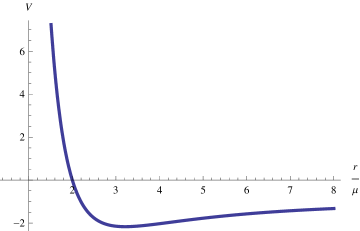
Figure 1: Plot of the anti-Schwarzschild potential $V(r/2\mu)$.

In Bonnor & Martins 1991 it is hinted that the non-existence of a clear newtonian limit is related to the existence of mass sources at $\infty$, but no definite conclusions were drawn.

IV The scalar-tensor solution

In order to derive the scalar-tensor generalization of the metric (6), we apply a theorem by Buchdahl Buchdahl 1959 establishing the reciprocity between any static solution of Einstein’s vacuum field equations and a one-parameter family of solutions of Einstein’s equations with a (massless) scalar field. The Einstein frame description of the scalar-tensor gravity theories fits into the conditions of the Buchdahl theorem. Indeed in this frame, after the conformal transformation of the original metric, we have GR plus a massless scalar field which is now coupled to the matter fields. Therefore, in the absence of matter we can use Buchdahl’s theorem and we are able to derive the scalar-tensor generalisation of the negatively curved metric we have been considering. Given the metric (6), we derive the corresponding scalar-tensor solution

$${\rm d}s^{2} = -\left(\frac{2\mu}{r}-1\right)^{B}\,{\rm d}t^{2}+\left(\frac{2\mu}{r}-1\right)^{-B}\;{\rm d}r^{2}$$

$$\qquad+\left(\frac{2\mu}{r}-1\right)^{1-B}\,r^{2}\,({\rm d}u^{2}+\sinh^{2}{u}\,{\rm d}v^{2})\,,$$

$$\varphi(r) = \sqrt{\frac{C^{2}(2\omega+3)}{16\pi}\varphi_{0}}\,\ln\left(\frac{2\mu}{r}-1\right)\;,$$ (18)

where

$$C^{2}=\frac{1-B^{2}}{2\omega+3}\qquad-1\leq B\leq 1\;.$$ (19)

This clearly reduces to our anti-Schwarzschild metric (6) in the GR limit when $B=1$, and hence $C=0$ implying that $G=\Phi^{-1}$ is constant (we assume $(2\omega+3)>0$ throughout). On the other hand this also shows that the solution has two branches corresponding to $C=\pm\{(1-B^{2})/(2\omega+3)\}^{1/2}$.

Notice that as pointed out by Agnese and La Camera Agnese:1985xj , the $r=2\mu$ limit is no longer just a coordinate singularity, but rather a true singularity as it can be seen from the analysis of the curvature invariants. In the spherically symmetric case, Agnese and La Camera show that the singularity at $r=2\mu$ has the topology of a point, and hence the event horizon of the black hole shrinks to a point. In the Einstein frame this happens because the energy density of the scalar field divergesDavid Wands 1993 . In the case under consideration the $r=2\mu$ condition now corresponds to the areal radius of the pseudo-spheres, $R=\left(\frac{2\mu}{r}-1\right)^{(1-B)/2}\,r$ becoming zero.

Reverting $\varphi=\int\sqrt{\Phi_{0}(2\omega+3)/(16\pi)}\,{\rm d}\ln(\Phi/\Phi_{0})$, and the conformal transformation, $g_{ab}=(2\mu/r-1)^{-C}\,\tilde{g}_{ab}$, we can recast this solution in the original frame in which the scalar-field is coupled to the geometry and the content is vacuum, i.e. the Jordan frame. We derive

$$\Phi(r) = \Phi_{0}\,\left(\frac{2\mu}{r}-1\right)^{C}\;,$$ (20)

$${\rm d}s^{2} = -\left(\frac{2\mu}{r}-1\right)^{B-C}\,{\rm d}t^{2}+\left(\frac{2\mu}{r}-1\right)^{-B-C}\;{\rm d}r^{2}$$ (21)

$$\qquad+\left(\frac{2\mu}{r}-1\right)^{1-B-C}\,r^{2}\,({\rm d}u^{2}+\sinh^{2}{u}\,{\rm d}v^{2})\,.$$

This shows that the gravitational constant $G=\Phi^{-1}$ decays from an infinite value at $r=0$ to a vanishing value at $r=2\mu$ when $C>0$, and conversely, grows from zero at $r=0$ to become infinite at $r=2\mu$, when $C>0$. As we did for the general relativistic case we study the geodesic behaviour of test particles in the scalar-tensor spacetime. The quantities $\epsilon$ and $h$ defined as the energy per unit mass and the angular momentum per unit mass, respectively, now become

$$\epsilon=\left(\frac{2\mu}{r}-1\right)^{B-C}\,\dot{t}\;\qquad,\qquad h=\left(\frac{2\mu}{r}-1\right)^{1-B-C}\,\left(r^{2}\,\sinh^{2}u_{\ast}\,\dot{v}\right)\;,$$ (22)

and are once again first integrals of the motion of test particles. Therefore for the “radial” motion of test particles, we have the following equation

$$\left(\frac{2\mu}{r}-1\right)^{-2C}\,\dot{r}^{2}+\left(\frac{2\mu}{r}-1\right)^{B-C}\,\left(1+\frac{h^{2}}{\left(\frac{2\mu}{r}-1\right)^{(1-B-C)}\,r^{2}\sinh^{2}u_{\ast}}\right)=\epsilon^{2}\;.$$ (23)

This is analogous to the equation of motion of a particle with variable mass under the potential $2V(r)=\left(\frac{2\mu}{r}-1\right)^{B-C}\,\left(1+\frac{h^{2}}{\left(\frac{2\mu}{r}-1\right)^{(1-B-C)}\,r^{2}\sinh^{2}u_{\ast}}\right)\;$. The latter crucially depend on the signs of the exponents of the terms $\xi(r)=\left(\frac{2\mu}{r}-1\right)\;.$ If we recast Eq. (23) as

$$\dot{r}^{2}+\xi^{B+C}\,\left(1+\frac{h^{2}}{\xi^{(1-B-C)}\,r^{2}\sinh^{2}u_{\ast}}\right)-\epsilon^{2}\,\xi^{2C}=0\,\;,$$ (24)

we now have the motion of a test particle with vanishing effective energy under the self-interaction potential

$$2V_{eff}(r)=\xi^{B+C}(r)\,\left(1+\frac{h_{\ast}^{2}}{r^{2}}\,\xi^{B+C-1}\right)-\epsilon^{2}\,\xi^{2C}\;,$$ (25)

where $h_{\ast}=h\sinh u_{\ast}$. In Figures 2 and 3 we plot some possible cases, which help us draw some important conclusions. On the one hand, high values of $\omega$ imply more repulsive potentials, since the higher $\omega$ the closer we are to GR. Notice that high values of $\omega$ mean small $C$, i.e., smaller variation of $G$. It is though remarkable that for larger departures from GR (left plot of 2) $V(r)$ may exhibit a minimum in the range $0<r<2\mu$, leading to closed orbits, something which was not possible in the GR solution. On the other hand comparing the left plots of Figures 2 and 3, we realise that the increase in angular momentum renders the potential more repulsive, shifting the minimum beyond $r=2\mu$.

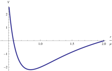
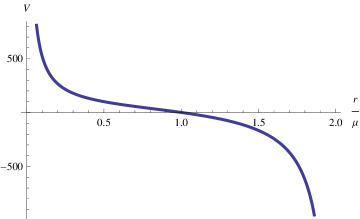
Figure 2: In both plots $\omega=0$, $B=1/2$, $h_{\ast}=1$, $\epsilon=2$, but left one has $C=+1/2$, and right $C=-1/2$.

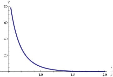
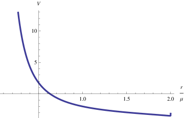
Figure 3: Left plot: $\omega=0$, $B=1/2=C$,$\epsilon=2$, but $h_{\ast}=2$, while right plot: $\omega=10^{4}$, $B=1/2$, $C=1/200$, $\epsilon=2$, $h_{\ast}=1$

Overall, what is most remarkable in what regards the vacuum ST solution derived here is that we are in the presence of a strong gravitational field. The absence of a newtonian asymptotic limit at the GR level is the signature of this situation, and prevents us from performing the usual PPN multipolar expansion that permits to identify the departures from GR. Thus, if one wishes to ascertain how our ST solution departs from GR, we need to look at the perturbation of the GR solution itself (rather than that of the almost Minkowski weak field solution). The way to accomplish this is to generalise the formalism developed in a number of remarkable works for the Schwarzschild solution (see Martel:2005ir and references therein). We have to trade the spherical symmetry of the latter by the pseudo-spherical symmetry of our solution. At present we are pursuing this task and we will report our results elsewhere. From the observational viewpoint what will be needed to test the admissibility of the negatively curved solutions under consideration (both the GR and the ST solutions) is to resort to test of strong fields requiring the detection of gravitational waves (for a discussion see Psaltis:2008bb )).

V Discussion

We have considered a static solution with a pseudo-spherical foliation of space. We reviewed its exotic features, and derived the extended scalar-tensor solution. The fundamental feature of these solutions is the absence of a newtonian weak field limit. Indeed it is known that not all of the GR solutions allow a newtonian limit, and this is the situation here. However, assuming that the solutions of the Einstein field equations represent gravitational fields, albeit far from our common physical settings, it is possible to ascertain the implications of varying $G$ in the strong fields by comparing the ST to their GR counterparts. From the viewpoint of observations this relies on the future detection of gravitational waves. We conclude with a quotation from John Barrow  Barrow:1991fj which seems appropriate here

The miracle of general relativity is that a purely mathematical assembly of second-rank tensors should have anything to do with Newtonian gravity in any limit.

References

- (1) C. M. Will, Living Rev. Rel. 9, 3 (2005). [gr-qc/0510072].
- (2) T. Damour, Astrophys. Space Sci. 283, 445-456 (2003). [gr-qc/0210059].
- (3) C. J. A. P. Martins, Nucl. Phys. Proc. Suppl. 194, 96-99 (2009).
- (4) J. D. Barrow, Phil. Trans. Roy. Soc. Lond. A363, 2139-2153 (2005). [astro-ph/0511440].
- (5) J. K. Webb, M. T. Murphy, V. V. Flambaum et al., Phys. Rev. Lett. 87, 091301 (2001). [astro-ph/0012539].
- (6) F. S. N. Lobo, [arXiv:0807.1640 [gr-qc]].
- (7) O. Bertolami, C. G. Boehmer, T. Harko et al., Phys. Rev. D75, 104016 (2007). [arXiv:0704.1733 [gr-qc]].
- (8) N. J. Nunes, T. Dent, C. J. A. P. Martins et al., [arXiv:0910.4935 [astro-ph.CO]].
- (9) Shin’ichi Nojiri, Sergei D. Odintsov ’Unified cosmic history in modified gravity: from F(R) theory to Lorentz non-invariant models’, [arXiv:1011.0544].
- (10) C. G. Boehmer, G. De Risi, T. Harko et al., Class. Quant. Grav. 27, 185013 (2010). [arXiv:0910.3800 [gr-qc]]
- (11) F. S. N. Lobo, J. P. Mimoso, Phys. Rev. D82, 044034 (2010). [arXiv:0907.3811 [gr-qc]].
- (12) C. Brans, R. H. Dicke, Phys. Rev. 124, 925-935 (1961).
- (13) T. Damour, K. Nordtvedt, Phys. Rev. D48, 3436-3450 (1993).
- (14) J. D. Barrow and J. P. Mimoso, Phys. Rev. D 50 (1994) 3746.
- (15) J. P. Mimoso and A. M. Nunes, Phys. Lett. A 248 (1998) 325.
- (16) J. P. Mimoso & A. Nunes, Astrophys. and Space Sci., 283 (2003) 661 .
- (17) J. P. Mimoso, D. Wands, Phys. Rev. D51, 477-489 (1995). [gr-qc/9405025].
- (18) J. O’Hanlon and B. O. J. Tupper, Il Nuovo Cimento 7, 305 (1972);
- (19) H. Stephani, D. Kramer, M. A. H. MacCallum, C. Hoenselaers and E. Herlt, “Exact solutions of Einstein’s field equations,” Cambridge, UK: Univ. Pr. (2003) 701 P
- (20) J. Ehlers and W. Kundt, “Exact Solutions of the gravitational Field Equation,” in Gravitation: an introduction to current research, ed. L. Witten, pp49 (Wiley, New York and London, 1962)
- (21) W. B. Bonnor and M- A. P. Martins, Classical and Quantum Gravity, 8, 727 (1991).
- (22) M. A. P. Martins, Gen. Rel. Grav. 28 (1996) 1309.
- (23) G. W. Gibbons,“Selfgravitating magnetic monopoles, global monopoles and black holes,” in Lecture notes in physics, 383, pp. 110-133, Berlin, Germany: Springer (1991)
- (24) L. A. Anchordoqui, J. D. Edelstein, C. Nunez and G. S. Birman, arXiv:gr-qc/9509018.
- (25) H. A. Buchdahl, Phys. Rev. 115, 1325 (1959).
- (26) D. Wands, Phd thesis, pp. 20, University of Sussex, 1993.
- (27) A. G. Agnese and M. La Camera, Phys. Rev. D 31 (1985) 1280.
- (28) J. P. Mimoso, F. S. N. Lobo, and N. Montelongo, “Dust solutions with pseudo-spherical symmetry,” in preparation.
- (29) K. Martel, E. Poisson, Phys. Rev. D71, 104003 (2005). [gr-qc/0502028].
- (30) D. Psaltis, ’Probes and Tests of Strong-Field Gravity with Observations in the Electromagnetic Spectrum’, [arXiv:0806.1531 [astro-ph]].
- (31) J. D. Barrow, Gravitation and Hot Big-Bang Cosmology, in Lecture notes in physics, 383, pp. 1-20, Berlin, Germany: Springer (1991)