Theory of non-equilibrium electronic Mach-Zehnder interferometer

Abstract

We develop a theoretical description of interaction-induced phenomena in an electronic Mach-Zehnder interferometer formed by integer quantum Hall edge states (with $\nu=1$ and 2 channels) out of equilibrium. Using the non-equilibrium functional bosonization framework, we derive an effective action which contains all the physics of the problem. We apply the theory to the model of a short-range interaction and to a more realistic case of long-range Coulomb interaction. The theory takes into account interaction-induced effects of dispersion of plasmons, charging, and decoherence. In the case of long-range interaction we find a good agreement between our theoretical results for the visibility of Aharonov-Bohm oscillations and experimental data.

I Introduction

Many recent experiments studied transport through an electronic analog of Mach-Zehnder interferometer (MZI) built on edge states in the quantum Hall regime heiblum03 ; heiblum06 ; heiblum07 ; heiblum07a ; roche07 ; roche08 ; roche09 ; strunk07 ; strunk08 ; strunk10 ; schoenenberger . These experiments show strong Aharonov-Bohm oscillations, which is a manifestation of quantum interference of electrons propagating along the arms of the interferometer. One of remarkable experimental observation is a lobe-type structure in the dependence of visibility on bias voltage. More precisely, the visibility strongly depends on voltage, showing decaying oscillations (“lobes”) characterized by certain energy scale. Such structure can not be explained within a model of non-interacting electrons (which would predict a constant visibility) and thus results from the electron-electron interaction. Therefore, the experiments on Mach-Zehnder interferometers exhibit the physics resulting from an interplay of a quantum interference and the Coulomb interaction under strongly non-equilibrium conditions. Development of a theory of such phenomena is a challenging task.

Various aspects of the relevant physics have been addressed in earlier works. Dephasing of quantum interference in Aharonov-Bohm rings, interferometers and related phenomena have been studied in many works for equilibrium aronov87 ; buettiker ; LeHur ; marquardt04 ; ludwig04 ; gornyi05 ; dmitriev10 and non-equilibrium neder07 ; gutman08 ; gutman10 ; NgoDinh10 setups. The importance of electron-electron interaction for the emergence of the lobe structure has been emphasized in Refs. sukhorukov07, ; Levkivskyi08, . In Ref. Chalker07, the influence of long-range ($1/r$) character of the Coulomb interaction (leading to a dispersion of the plasmon mode) was analyzed. In the works neder08, ; youn08, ; kovrizhin09, a simplified model with a quantum-dot-type treatment of the interaction was solved.

The goal of the present article is to present a systematic theory of transport in a non-equilibrium quantum Hall Mach-Zehnder interferometer and to confront its predictions with the experiment. This theory formulated in terms of functional-bosonization Keldysh action in Sec. II takes into account all effects of the electron-electron interaction, including formation and characteristics of the lobe structure, as well as the dephasing. In Sec. III we apply the theory to the model of short-range interaction. In this way we reproduce the earlier results on the lobe structure Levkivskyi08 and also find the suppression of the interference signal due to dephasing. While showing some similarity to experimental observations, the results of the short-range-interaction model contradict to the experiment in several crucial aspects. This motivates us to explore the more realistic case of $1/r$ Coulomb interaction in Sec. IV. Using our general formalism, we analyze the cases of $\nu=1$ and $\nu=2$ edge modes. The obtained parametric dependences of the interference signal are in good agreement with experiments, although in the case of $\nu=1$ mode some discrepancies remain. We summarize our findings and discuss further research directions in Sec. V.

II General framework

II.1 Model and the functional bosonization

We consider a theoretical model of the Mach-Zehnder interferometer, realized with edge states in the quantum Hall regime at filling fraction $\nu=1$ and $\nu=2$, as schematically shown in Figs. 1 and 2. The outer channels propagating along different arms (index: $\pm$) of the interferometer are coupled by means of two quantum point contacts (QPCs), located at points $x_{1}^{\pm}$ and $x_{2}^{\pm}$. Each QPC can be generally described by the unitary $2\times 2$ scattering matrix

$$S_{j}=\left(\begin{array}[]{cc}ir_{j}&\tau_{j}\\ \tau_{j}&ir_{j}\end{array}\right)\>,\ \ \ j=1,2\>,$$ (1)

where the transmission and reflection coefficients, $\tau_{j}$ and $r_{j}$ are assumed to be real. In case of $\nu=2$ this scattering matrix relates incoming modes of two outer channels (in up/down arms) with the outgoing ones. Electrons in the inner channels are assumed to propagate through the QPCs without scattering.

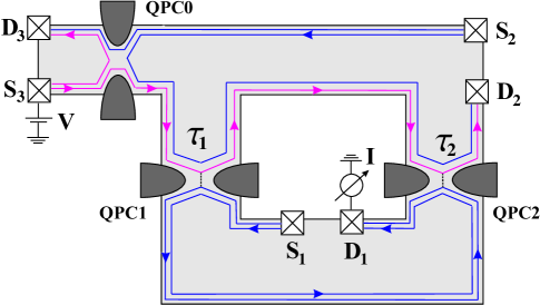
Figure 1: Scheme of an electronic Mach-Zehnder interferometer built on quantum-Hall edge states at filling factor $\nu=2$. Quantum point contact (QPC1 and QPC2) characterized by transmission amplitudes $\tau_{1(2)}$ are used to partially mix the outer edge channels. All Ohmic contacts are grounded, except for the source terminal $S_{3}$ which is kept at voltage $V$. The current is measured in the drain terminal $D_{1}$. The QPC0 is pinched in such a way that the inner channel is completely reflected while the outer one is fully transmitted.

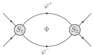
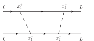
Figure 2: Top: Schematics of a Mach-Zehnder interferometer. Two quantum point contacts are characterized by scattering matrices $S_{1}$ and $S_{2}$. The electron-electron interaction is decoupled via a Hubbard-Stratonovich fields $\varphi^{+}$ and $\varphi^{-}$ on two arms of the interferometer. Bottom: Coordinates on two arms of the interferometer.

The arms of the interferometer can be different, thereby generally $x_{j}^{+}\neq x_{j}^{-}$. The coordinates $L^{\pm}$ and $0$ refer to the points where the MZI is connected to the drain and source reservoirs. Specifying the non-equilibrium boundary conditions, we assume that only one single channel is biased at the chemical potential $eV$, while all others are grounded. In case of $\nu=2$ it will be the outer upper channel, as shown in Fig. 1. In the experiments heiblum06 ; roche07 ; strunk08 such situation is realized with the use of an extra QPC which splits the incoming inner and outer channels [see Fig. 1], so that these channels originate from different reservoirs.

To set the stage, we start by considering the simplest situation, when $r_{j}=1$ and $\tau_{j}=0$, so that outer channels in the two arms of the interferometer are completely decoupled from each other. In this case we model the system by a set of interacting chiral fermions with the action ${\cal S}={\cal S}_{0}+{\cal S}_{\rm int}$, where

$${\cal S}_{0} = -iv\sum_{\alpha}\int dt\,dx\,\psi^{*}_{\alpha}(x)\partial_{x}\psi_{\alpha}(x),$$ (2)

$${\cal S}_{\rm int} = {1\over 2}\sum_{\alpha}\int dt\,dxdx^{\prime}\rho_{\alpha}(x)U_{0}(x-x^{\prime})\rho_{\alpha}(x^{\prime})\,.$$

Here $\psi_{\alpha}$ is a Grassmann field of the chiral fermion in the arm $\alpha=\pm$. In case of $\nu=2$ it has the vector structure $\psi_{\alpha}=(\psi_{1\alpha},\psi_{2\alpha})^{T}$, the subscript $p=1,2$ denoting the outer and the inner channels, respectively. The potential $U_{0}$ describes the bare interaction within the interferometer arm between the chiral electron densities

$$\rho_{\alpha}(x)=\,\psi^{*}_{\alpha}(x+0)\psi_{\alpha}(x),$$

and $v$ denotes the drift velocity in the edge.

In what follows we are going to use the Keldysh version of the functional bosonization lerner04 . Let us recall the basic ideas of this construction. We decouple the interaction term ${\cal S}_{\rm int}$ using the Hubbard-Stratonovich transformation with a field $\varphi$ and double the number of fields; $\psi=(\psi_{f},\psi_{b})^{T}$ (and the same for $\varphi$), where $\psi_{f(b)}$ denote the Grassmann fields residing at the forward (backward) branch of the Keldysh contour. These steps lead us to the action

$$\mathcal{A} = \sum_{\alpha}\left[\int_{{\cal C}_{K}}dtdx\,\psi^{*}_{\alpha}(i\partial_{t}+iv\partial_{x}-\varphi_{\alpha})\psi_{\alpha}\right.$$ (3)

$$+ \left.\frac{1}{2}\int_{{\cal C}_{K}}dtdxdx^{\prime}\,\varphi_{\alpha}U_{0}^{-1}(x-x^{\prime})\varphi_{\alpha}\right]\>,$$

where we assume the implicit summation over the channel indices.

The minimal coupling between fermionic and bosonic degrees of freedom in 1D geometry can be eliminated by a local gauge transformation, $\psi_{\alpha}\rightarrow\psi_{\alpha}e^{i\Theta_{\alpha}}$, if one requires that

$$(\partial_{t}+v\partial_{x})\,\Theta_{\alpha}=-\varphi_{\alpha}.$$ (4)

One has to resolve this differential equation by taking the proper structure of the Keldysh theory into account,

$$\left(\begin{array}[]{c}\Theta_{f}\\ \Theta_{b}\end{array}\right)_{\xi}=-\int d\xi^{\prime}\left(\begin{array}[]{cc}D_{0}^{T}&D_{0}^{<}\\ D_{0}^{>}&D_{0}^{\tilde{T}}\end{array}\right)_{\xi-\xi^{\prime}}\left(\begin{array}[]{c}\varphi_{f}\\ -\varphi_{b}\end{array}\right)_{\xi^{\prime}}.$$ (5)

Here we have denoted $\xi\equiv(x,t)$ and omitted the arm/channel indicies for brevity. At zero temperature elements of the bare particle-hole propagator $\hat{D}_{0}$ in the space-time representation are given by the relations

$$D^{\gtrless}_{0}(\xi) = v^{-1}\,n_{B}^{\gtrless}(t-x/v),$$

$$D^{T/\tilde{T}}_{0}(\xi) = \theta(\mp t)D^{<}_{0}(\xi)+\theta(\pm t)D^{>}_{0}(\xi),$$ (6)

where $n_{B}^{\gtrless}(t)=-i/2\pi(t\mp ia/v)$, $\theta(t)$ is the Heaviside theta-function and $a$ is a short (ultraviolet) cutoff scale that is of the order of magnetic length $l_{B}$. After this gauge transformation the Green function of interacting electron acquires the form

$$G^{>}(\xi_{1},\xi_{2})=g^{>}(\xi_{1}-\xi_{2})\langle e^{i\Theta_{b}(\xi_{1})}e^{-i\Theta_{f}(\xi_{2})}\rangle_{\mathcal{A}_{0}}\,.$$ (7)

Here $g^{>}(\xi)$ is the free zero-temperature Green function,

$$g^{>}(\xi)=\frac{1}{2\pi v}\frac{e^{-i(t-x/v)eV}}{(x/v-t+ia/v)}$$ (8)

that should be understood as a diagonal $4\times 4$ (two arms, two channels) matrix; for the sake of generality, we assume that at $\nu=2$ channels are biased by distinct voltages $V_{p}^{\alpha}$, where $p=1,2$ is the channel index, and $\alpha=\pm$ is the arm index. The average over phases $\Theta(\xi)$ in Eq. (7) is performed with the Gaussian action

$$\mathcal{A}_{0}(\varphi)=\frac{1}{2}\vec{\varphi}^{\,t}U_{0}^{-1}\sigma_{z}\vec{\varphi}-\frac{1}{2}\vec{\varphi}^{\,t}\Pi\vec{\varphi}-\vec{\varphi}^{\,t}\sigma_{z}\rho_{0},$$ (9)

which is a special property of the 1D geometry (Larkin-Dzyaloshinskii theorem). Written in the symbolic form, this expression implies the summation over the Keldysh indices (determining the vector structure of $\vec{\varphi}$) and convolution in the space/time domain, see Eq. (5). The matrix $\Pi$ is the polarization operator ($a,a^{\prime}$ denoting the Keldysh indices)

$$\Pi^{aa^{\prime}}(\xi)=-ig^{aa^{\prime}}(\xi)g^{a^{\prime}a}(-\xi)-(2\pi v)^{-1}\delta(\xi)\,a\,\delta^{aa^{\prime}},$$ (10)

with the last term accounting for the static compressibility of edge channels. The linear in $\varphi$ term in the action (9) describes the response of the system to the external non-equilibrium charge $\vec{\rho}^{\,t}\equiv(\rho_{0},\rho_{0})$ injected from the leads

$$\rho_{0}(\xi)=(2\pi v)^{-1}eV(\,t-x/v).$$ (11)

It is convenient to perform the Keldysh rotation (see e.g., Ref.Kamenev99, ), introducing the “classical” and “quantum” components of the fields

$$\varphi_{c(q)}=(\varphi_{f}\pm\varphi_{b})/2,$$ (12)

Then the polarization operator in the frequency-momentum representation acquires the Keldysh structure with

$$\Pi_{R,A}=-\frac{\nu}{2\pi}\frac{q}{qv-\omega\mp i0};$$

$$\Pi_{K}=(\Pi_{R}-\Pi_{A})\coth(\beta\omega/2).$$ (13)

Minimizing the action (9), $\delta\mathcal{A}_{0}(\varphi)/\delta\varphi_{q}=0$, one obtains the linear equations for the mean value of a classical electrostatic field $\bar{\varphi}_{c}$ and an induced charge $\rho_{i}$ at the edge,

$${U}_{0}^{-1}(q)\bar{\varphi}_{c}=\rho_{i}+\rho_{0},$$

$$\rho_{i}={\Pi}_{R}(q,\omega)\bar{\varphi}_{c}.$$ (14)

Below we concentrate on the experimental situation with a dc applied voltage which introduces a homogeneous charge, so that we can take the limit $\omega=0$, $q\sim 1/L$, with $L$ being the system size.

Evaluation of the Green function (7) is now reduced to a Gaussian integral:

$$G^{>}(\xi,\xi^{\prime})=g^{>}(\xi-\xi^{\prime})\exp\left\{i[\bar{\Theta}(\xi)-\bar{\Theta}(\xi^{\prime})]-J^{>}(\xi-\xi^{\prime})\right\},$$ (15)

where the average phase $\bar{\Theta}$ is induced by the mean classical electrostatic field

$$\bar{\Theta}(\xi)=-v^{-1}\int_{0}^{x}dx^{\prime}\,\bar{\varphi}_{c}(x^{\prime},t+(x^{\prime}-x)/v),$$ (16)

and $J$ is the correlation function of the Gaussian phase fluctuations $\delta\Theta$ around the above mean value:

$$J^{aa^{\prime}}(\xi)=\frac{1}{2}\langle[\,\delta\Theta^{a}(\xi)-\delta\Theta^{a^{\prime}}(0)]^{2}\rangle_{\mathcal{A}_{0}}\,.$$ (17)

The phase-phase correlation function can be expressed in terms of the bare particle-hole propagator $D_{0}$ and the effective interaction

$$\langle\vec{\varphi}\vec{\varphi}^{\,t}\rangle=\frac{i}{2}{\cal U}=\frac{i}{2}(\sigma_{z}U_{0}^{-1}-\Pi)^{-1}\,.$$ (18)

Using the linear relation (5) between the phase and the electrostatic potential, one obtains

$$J^{aa^{\prime}}(\xi)={\cal D}^{aa^{\prime}}(\xi)-{\cal D}^{aa^{\prime}}(0),$$ (19)

where

$${\cal D}=D_{0}{\cal U}D_{0}.$$ (20)

The correlation function $J^{aa^{\prime}}(\xi)$ can be now easily evaluated with the use of $(\omega,q)$ representation. The result reads

$$J^{aa^{\prime}}(\xi)={\nu}^{-1}\left(J^{aa^{\prime}}_{P}(\xi)-J^{aa^{\prime}}_{F}(\xi)\right),$$ (21)

where we decomposed $J(\xi)$ into plasmon (P) and free (F) parts,

$$J^{>}_{P/F}(x,t)=\int_{0}^{\infty}\frac{dq}{q}\left[1-e^{iqx-iu_{P/F}(q)qt}\right]e^{-aq},$$ (22)

with the plasmon velocity

$$u_{P}(q)=v+\nu U_{0}(q)/(2\pi)$$ (23)

and the drift velocity $u_{F}=v$, respectively. Equation (21) is the zero temperature result for the “greater” function. The “lesser” correlation functions satisfies $J^{<}(\xi)=[J^{>}(\xi)]^{*}$, and the (anti-) time-ordered correlators can be reconstructed with the use of basic definitions, akin to Eq. (6).

Equation (22) yields for $J_{F}^{>}$:

$$J_{F}^{>}(\xi)=\ln{x-vt+ia\over ia}\,.$$ (24)

Thus, in the case $\nu=1$ the bare electron pole in Eq. (7) is canceled by the free contribution to $J(\xi)$ and the electron motion is determined solely by the plasmon contribution, whereas for $\nu=2$ both plasmon and free (neutral) modes do influence the behavior of electronic propagator. The plasmon contribution $J_{P}(\xi)$ depends on the specific form of the electron-electron interaction through the momentum dispersion in the velocity $u_{P}(q)$. We consider two models of short-range, $U_{0}(x)\propto\delta(x)$, and long-range, $U_{0}(x)\propto 1/|x|$, interactions in the following Sections III and IV.

II.2 Keldysh action of the Mach-Zehnder interferometer

In this section we generalize the discussion of the functional bosonization to include electron scattering at QPCs which are crucial elements of the MZI layout. In this way we construct the most general Keldysh action ${\cal A}(\varphi)$ of the MZI, which is applicable for arbitrary scattering matrices characterizing two QPCs. The Keldysh action can be expressed in terms of a total single-particle time-dependent interferometer scattering matrix $S(t,t^{\prime},[\varphi])$. It describes scattering of electrons at QPCs as well as their propagation along the arms of the interferometer in the fluctuating Hubbard-Stratonovich field $\varphi$. The $S$-matrix is thus non-local in time and takes different values ($S_{f}=S[\varphi_{f}]$ and $S_{b}=S[\varphi_{b}]$ ) on the forward (backward) branch of the Keldysh contour, since the fields $\varphi_{b}(x,t)$ and $\varphi_{f}(x,t)$ generally differ. The action ${\cal A}(\varphi)$ has the form

$$i\mathcal{A}(\varphi,\vec{\chi}) = \ln\det\left[1+(S_{b}^{\dagger}e^{i\hat{\chi}}S_{f}-1)\hat{f}\right]-i\vec{\varphi}^{\,t}\,\tilde{\Pi}\,\vec{\varphi}\,$$ (25)

$$+ i\vec{\varphi}^{\,t}U_{0}^{-1}\sigma_{x}\vec{\varphi}.$$

Here $\vec{\varphi}=(\varphi_{c},\varphi_{q})^{t}$ is assumed to be written in the Keldysh basis. We have also introduced the electron distribution function in the source reservoirs, $\hat{f}=\mathrm{diag}(f^{+},f^{-})$ (in the case $\nu=2$ each $f^{\pm}$ is itself a diagonal matrix in the channel space with the components $f_{p}^{\pm}$), and auxiliary “counting fields” $\hat{\chi}=\mathrm{diag}(\chi^{+},\chi^{-})$ in the drains which enable us to find the number of transferred electrons. The determinant in Eq. (25) is evaluated with respect to time, arm, and channel indices. Since in this paper we restrict ourselves to the case of zero temperature, the distribution functions in time domain read

$$f_{p}^{\pm}(t,t^{\prime})=-\frac{e^{-ieV_{p}^{\pm}(t-t^{\prime})}}{2\pi i(t-t^{\prime}+i0)},$$ (26)

where $V_{p}^{\pm}$ correspond to voltages applied to the different channels. The polarization operator $\tilde{\Pi}$ has the form

$$\tilde{\Pi}=\left(\begin{array}[]{cc}0&\Pi_{A}\\ \Pi_{R}&0\end{array}\right).$$ (27)

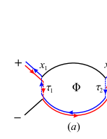
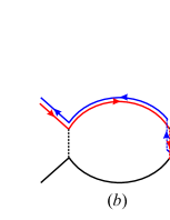
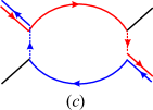
Figure 3: Example of paths contributing to the matrix element $R=Q_{++}$. The paths (a) and (b) give direct contributions, while the path (c) encloses the magnetic flux $\Phi$ and describes the interference process. The corresponding analytical expressions read: (a) $\tau_{1}^{2}\tau_{2}^{2}\Gamma_{1}^{\dagger b}\Gamma_{2}^{b}\Gamma_{2}^{\dagger f}\Gamma_{1}^{f}$; (b) $r_{1}^{2}\tau_{2}^{2}\Gamma_{2}^{\dagger b}\Gamma_{2}^{f}e^{-i\chi}$; (c) $r_{1}r_{2}\tau_{1}\tau_{2}\Gamma_{1}^{\dagger b}\Gamma_{2}^{f}e^{i\Phi}e^{-i\chi}$.

We now specify the total scattering matrix $S$ for the MZI. It can be decomposed into the scattering matrices of the quantum point contacts (QPC), $S_{1}$ and $S_{2}$, and the transfer matrices accounting for the propagation from $0$ (“source”) to $x_{1}$ ($T_{10}$), from $x_{1}$ to $x_{2}$ ($T_{21}$) and from $x_{2}$ to $L$ ($T_{L2}$) (“drain”) (see Fig. 2),

$$S=T_{L2}S_{2}T_{21}S_{1}T_{10}\,.$$ (28)

with the scattering matrices of the contacts defined by Eq. (1). Since the Hubbard-Stratonovich field is diagonal in the channel space, the transfer matrix can be written as

$$T_{ji}(t,t^{\prime})=\Lambda_{ji}(t,t^{\prime})e^{i\theta_{ji}(t^{\prime})},$$ (29)

where the shift operator

$$\Lambda^{\pm}_{ji}(t,t^{\prime})=\delta(t-t^{\prime}-(x_{j}^{\pm}-x_{i}^{\pm})/v)$$ (30)

describes the free propagation, and

$$\theta^{\pm}_{ji}(t)=-v^{-1}\int_{x_{i}^{\pm}}^{x_{j}^{\pm}}dx^{\prime}\varphi^{\pm}(x^{\prime},t+(x^{\prime}-x_{i}^{\pm})/v)$$ (31)

is the electron phase induced by the Hubbard-Stratonovich field during the propagation of an electron from $x_{i}$ to $x_{j}$. The weak variation of magnetic field gives rise to an additional Aharonov-Bohm phase $\Phi=\Phi_{+}-\Phi_{-}$, which we incorporate by $\theta_{21}^{\pm}\rightarrow\theta_{21}^{\pm}+\Phi^{\pm}$. Definition (28) gives both $S_{f}$ and $S_{b}$ depending on weather $\varphi_{f}$ or $\varphi_{b}$ is used to reconstruct the electron phase in Eq. (31). We note, that the phase $\theta_{f/b}^{\pm}$, considered as the function of $(x_{j},t)$, satisfies Eq. (4). However, this phase is different from $\Theta_{f/b}^{\pm}$, because the relation (31) does not contain information about Keldysh distribution functions, as opposed to Eq. (5).

The cumulant generating function of the MZI can be now expressed as a functional integral over $\varphi$,

$${\cal Z}(\vec{\chi})=\int{\cal D}\varphi_{f/b}^{\pm}(x,t)\,\exp\left\{i{\cal A}(\,\varphi,\vec{\chi})\right\}.$$ (32)

In particular, it gives the mean number of transferred charges to the upper/lower drains,

$$N^{\pm}=-i\partial_{\chi^{\pm}}\ln{\cal Z}(\vec{\chi})|_{\vec{\chi}=0}.$$ (33)

A detailed derivation of the action (25) will be published elsewhere NgoDinh . This action bears connection with the solution of the problem of full counting statistics Levitov93 ; counting-statistics . Related Keldysh actions of the determinant structure were found for the problems of a local scatterer in Ref. Snyman08, and of a quantum wire in Ref. gutman10, . One can also show that in the limit of zero tunneling, $\tau_{i}=0$, the full action (25) is reduced to the Gaussian one, given by Eq. (9). In this case the linear in $\varphi$ term and the classical Gaussian fluctuations of $\varphi$, described by $\Pi_{K}$ [see Eq.(13)], happen to be the first two terms in the expansion of the functional determinant of the action (25), while the higher order terms in $\varphi$ vanish.

In general, the integral over the Hubbard-Stratonovich field with the determinant action ${\cal A}(\varphi)$ can not be evaluated analytically. In the following, we proceed with the analysis of the MZI in the weak tunneling limit, $\tau_{j}\ll 1$. Since in the absence of tunneling the MZI is described by the Gaussian action (9), we can introduce the tunneling action ${\cal A}_{t}(\varphi)$, so that ${\cal A}(\varphi)={\cal A}_{0}(\varphi)+{\cal A}_{t}(\varphi)$, where the expansion of ${\cal A}_{t}$ in terms of $\tau_{j}$ starts from the terms of order of ${\cal O}(\tau^{2})$. In Appendix A we show that the tunneling action ${\cal A}_{t}$ can be obtained by a proper regularization of the functional determinant appearing in Eq. (25), yielding

$$i\mathcal{A}_{t}=\ln\det\left[1+\left(e^{i\tilde{\psi}_{b}}S_{b}^{\dagger}(\chi)S_{f}(\chi)e^{-i\tilde{\psi}_{f}}-1\right)\bar{f}\right]\,.$$ (34)

Here

$$S_{f}(\chi)=e^{i\hat{\chi}/2}S_{f}e^{-i\hat{\chi}/2},\quad S_{b}^{\dagger}(\chi)=e^{-i\hat{\chi/2}}S_{b}^{\dagger}e^{i\hat{\chi/2}},$$ (35)

and

$$\tilde{\psi}^{\pm}_{f,b}(t)=-v^{-1}\int_{0}^{L^{\pm}}dx^{\prime}\varphi^{\pm}_{f,b}(x^{\prime},t+x^{\prime}/v)$$ (36)

is the phase collected along the way from $0$ to $L^{\pm}$ without tunneling. In other words, $\tilde{\psi}^{\pm}$ is equal to $\theta_{ij}^{\pm}$ with $x_{i}=0$ and $x_{j}=L^{\pm}$. New distribution functions $\bar{f}^{\pm}_{\alpha}$ are obtained from the original distribution functions in the sources (26) with the use of a gauge transformation,

$$\bar{f}(t,t^{\prime}) = e^{i\hat{\lambda}(t)}\hat{f}(t,t^{\prime})e^{-i\hat{\lambda}(t^{\prime})},$$ (37)

$$\hat{\lambda}^{\pm}_{\alpha}(t) = f_{>}\tilde{\psi}_{f,\alpha}^{\pm}+f_{<}\tilde{\psi}_{b,\alpha}^{\pm},$$ (38)

where we defined the projectors on the hole and particle subspaces

$$f_{\gtrless}(t-t^{\prime})=\pm 1/2\pi i(t-t^{\prime}\mp i0)$$ (39)

(see also Appendix A). According to our general notational conventions, Eq. (38) has to be understood as a convolution in time domain.

To proceed with the evaluation of the tunneling action, we introduce a matrix (in the time, arm, and channel space)

$$Q=e^{i\tilde{\psi}_{b}}S_{b}^{\dagger}(\chi)S_{f}(\chi)e^{-i\tilde{\psi}_{f}}=\left(\begin{array}[]{cc}R&T\\ T^{\prime}&R^{\prime}\end{array}\right).$$ (42)

The second equation in Eq. (42) introduces a block decomposition of $Q$ in the arm space. In the absence of tunneling $Q(t,t^{\prime})=\delta(t-t^{\prime})$ and ${\cal A}_{t}$ vanishes. Since the tunneling affects only outer channels, it is sufficient to keep only the corresponding elements of the matrix $Q$. Therefore, from now on $Q$ is the matrix in the arm and time space only, both for $\nu=1$ and $\nu=2$ setups.

To find $Q$ in the presence of tunneling we define the “hopping” operators at each QPC,

$$\Gamma_{i}^{f/b}(t,t^{\prime})=e^{i{\theta}_{Li}^{-,f/b}(t)}\delta(t-t^{\prime}-(x_{i}^{+}-x_{i}^{-})/v)\,e^{-i{\theta}_{Li}^{+,f/b}(t^{\prime})},$$ (43)

where ${\theta}_{Li}^{\alpha,f/b}(t)$ is the phase picked up by the electron along the path from $x_{i}$ to the drain $\alpha$, as given by the relation (31). We can further formulate a set of simple rules that enable one to express the matrix elements $Q_{\alpha\beta}$ in terms of these operators:

• Each matrix element $Q_{\alpha\beta}$ is associated with a number of possible continuous paths that originate from the source terminal $\alpha$, go to any of the drain terminals and return back to the source $\beta$ (see Fig. 3). The forward and backward paths are allowed to go through the different interferometer arms. In the latter case the associated contribution corresponds to the interference process. Each element $Q_{\alpha\beta}$ is thus a sum of eight contributions.

• Each transmission via QPC $j$ gives the factor $\tau_{j}$. Each reflection gives the factor $\pm ir_{j}$ along the forward/backward path respectively.

• Each tunneling process from arm $+$ to $-$ which happens at the QPC $j$ is associated with the amplitude $\hat{\Gamma}_{i}^{f/b}e^{\mp i\chi/2}$, where $\chi=\chi_{+}-\chi_{-}$. The inverse tunneling process is described by the Hermitian conjugate of this operator. The product of such “hopping” operators must be path-ordered.

• contributions associated with the interference process carry the extra Aharonov-Bohm phase $e^{\pm i\Phi}$.

As an example, three (out of eight) contributions to the matrix element $R=Q_{++}$ are shown in Fig. 3. The full analytical expressions for $Q_{\alpha\beta}$ is presented in Appendix B. The next step is to use the expansion

$$i\mathcal{A}_{t}=\mathrm{Tr}\left((Q-1)\bar{f}-\frac{1}{2}\left((Q-1)\bar{f}\,\right)^{2}\right)+\mathcal{O}(\tau^{3})\,.$$ (44)

Some important technical details of the evaluation of ${\cal A}_{t}$ with the use of this formula are given in Appendix C. We show there that the second-order approximation in $\tau_{j}$ for the tunneling action $\mathcal{A}_{t}$ has a form

$$i\mathcal{A}_{t} = \sum_{ij}\tau_{i}\tau_{j}$$

$$\times \int_{{\cal C}_{K}}dt_{1,2}\,e^{i\Theta(x_{i},t_{1})}\Pi_{ij}(t_{1},t_{2})e^{-i\Theta(x_{j},t_{2})}.$$

Here the summation is performed with respect to QPC indices ($i,j=1,2$) and the time integration goes along the Keldysh contour. The generalized polarization operators for the direct terms read

$$\Pi_{ii}^{T/\tilde{T}}(t_{1},t_{2}) = -\,f^{+}_{>,<}(t_{1}-t_{2})f^{-}_{<,>}(t_{2}-t_{1})\,,$$

$$\Pi_{ii}^{\gtrless}(t_{1},t_{2}) = \Pi_{ii}^{T/\tilde{T}}(t_{1},t_{2})\,e^{\pm i\chi},\quad$$ (46)

and the polarization operators of the interference terms are given by

$$\Pi_{12}^{T/\tilde{T}}(t_{1},t_{2}) = -e^{-i\Phi}f^{+}_{<,>}\left(t_{1}-t_{2}-(x_{1}^{+}-x_{2}^{+})/v\right)$$

$$\times f^{-}_{>,<}\left(t_{2}-t_{1}-(x_{2}^{-}-x_{1}^{-})/v\right)\,,$$

$$\Pi_{12}^{\gtrless}(t_{1},t_{2}) = \Pi_{12}^{\tilde{T}/T}(t_{1},t_{2})\,e^{\pm i\chi},$$ (47)

$$\Pi_{21}^{T/\tilde{T}}(t_{1},t_{2}) = -e^{i\Phi}f^{+}_{>,<}\left(t_{1}-t_{2}-(x_{2}^{+}-x_{1}^{+})/v\right)$$

$$\times f^{-}_{<,>}\left(t_{2}-t_{1}-(x_{1}^{-}-x_{2}^{-})/v\right)\,,$$

$$\Pi_{21}^{\gtrless}(t_{1},t_{2}) = \Pi_{21}^{T/\tilde{T}}(t_{1},t_{2})\,e^{\pm i\chi}.\quad$$ (48)

They are built up from the electron and hole distribution functions

$$f_{\gtrless}^{\pm}(t-t^{\prime})=e^{-ieV^{\pm}(t-t^{\prime})}f_{\gtrless}(t-t^{\prime}).$$ (49)

The polarization operators are dressed by relative gauge factors $\Theta(x_{i},t)=\Theta^{+}(x_{i}^{+},t)-\Theta^{-}(x_{i}^{-},t)$, where the phases $\Theta^{\pm}$ at each arms $\pm$ are linked to the corresponding HS-field $\varphi^{\pm}$ by relation (5), thereby taking the interaction into account.

The structure of the polarization operators can be interpreted as follows. The component $\Pi^{<}\propto f^{+}_{<}f^{-}_{>}$ corresponds to a particle excitation in the arm $+$ and a hole excitation in the arm $-$. This implies the charge transfer from $+$ to $-$, which explains the “counting” factor $e^{-i\chi}$. Similar considerations explain the structure of $\Pi^{>}$. Finally, the components $\Pi^{T/\tilde{T}}$ at $\chi=0$ are related to $\Pi^{\gtrless}$ via the conventional Keldysh-formalism relations, $\Pi^{T/\tilde{T}}\bigl{|}_{\chi=0}(t)=\theta(t)\Pi^{\gtrless}(t)+\theta(-t)\Pi^{\lessgtr}(t)$.

II.3 Gaussian approximation

The Keldysh action enables us to calculate the tunneling current of the interferometer. Specifically, let us consider the current of particles transported from the upper ($+$) to the lower interferometer arm ($-$). This current can be obtained as derivative of the cumulant generating function ${\cal Z}(\vec{\chi})$ with respect to $\chi_{-}$. We express the current as difference of up- and down rates, $I=\sum_{ij}(I_{ij}^{<}-I_{ij}^{>})$, with

$$I_{ij}^{<,>}=-\frac{e}{t_{0}}\tau_{i}\tau_{j}\int_{-\infty}^{\infty}dt_{1}dt_{2}\Pi_{ij}^{<,>}(t_{1},t_{2})$$

$$\times\left\langle e^{i\Theta^{f,b}(x_{i},t_{1})}e^{-i\Theta^{b,f}(x_{j},t_{2})}\right\rangle_{\mathcal{A}_{0}+\mathcal{A}_{t}(\chi=0)}\,,$$ (50)

where we introduced the measurement time $t_{0}$. The average over phases is to be done with the full action. However, to the leading approximation, we can neglect the tunneling action and perform the phase average with the Gaussian action ${\cal A}_{0}$. The corresponding correlation functions of phase variables are given by Eq. (21). Assuming that no interaction is present between the different interferometer arms, we find

$$I_{ij}^{\gtrless} = e\tau_{i}\tau_{j}v^{2}$$

$$\times \int dtG^{+,\gtrless}(x_{i}^{+}-x_{j}^{+},t)G^{-,\lessgtr}(x_{j}^{-}-x_{i}^{-},-t)\,,$$

where the full Green functions are given by Eq. (15). Equation (II.3) was the starting point of the discussion in the works by Chalker, Gefen and Veillette Chalker07 and Levkivskyi and Sukhorukov Levkivskyi08 . We go beyond it by including into consideration the (non-Gaussian) tunneling action that controls the non-equilibrium dephasing.

II.4 Non-Gaussian effects

Let us now improve the result for the tunneling current (II.3) by taking into account the non-Gaussian nature of phase fluctuations, which are described by the tunneling part of the action ${\cal A}_{t}$. These fluctuations are responsible for the intrinsic dephasing in the MZI by the non-equilibrium shot noise generated in the QPCs. To be specific, we evaluate $I_{ij}^{<}$, which requires calculation of the correlation function

$$\left\langle e^{i\Theta^{f}(x_{i},t_{1})}e^{-i\Theta^{b}(x_{j},t_{2})}\right\rangle=\int\mathcal{D}\varphi e^{i\mathcal{A}^{<}_{ij}+i\mathcal{A}_{0}+i\mathcal{A}_{t,\chi=0}},$$ (52)

where we have introduced a linear-in-$\varphi$ term in the action,

$$\mathcal{A}^{<}_{ij}(t_{1},t_{2},[\varphi]) = \Theta^{f}(x_{i},t_{1})-\Theta^{b}(x_{j},t_{2})$$ (53)

$$= \sum_{\alpha}\int dtdx(\vec{\Theta}^{\alpha})^{t}\vec{\cal J}^{\alpha}.$$

Here $\vec{\cal J}^{\pm}=({\cal J}^{\pm,f},{\cal J}^{\pm,b})^{t}$ are source terms acting on both branches of the Keldysh contour,

$$\mathcal{J}^{\pm,f}(x,t) =\pm\delta(x-x^{\pm}_{i})\delta(t-t_{1}),$$

$$\mathcal{J}^{\pm,b}(x,t) =\mp\delta(x-x^{\pm}_{j})\delta(t-t_{2}).$$ (54)

In order to account for the non-Gaussian effects, we proceed with a real-time instanton approach developed in Ref. NgoDinh10, for the problem of tunneling spectroscopy of a biased quantum wire with a scatterer. We look for the optimal (saddle-point) trajectory $\varphi^{\alpha}_{*}(x,t)$, which minimizes the total action $\mathcal{A}_{\rm tot}=\mathcal{A}_{0}+\mathcal{A}_{t}+\mathcal{A}_{ij}^{<}$ at $\chi=0$. In the weak tunneling limit, $\tau_{j}\ll 1$, one can find the instanton trajectory $\varphi^{*}$ approximately by minimizing only the quadratic part of the action, i.e. $\mathcal{A}_{0}+\mathcal{A}_{ij}^{<}$. This yields for the stationary point

$$\vec{\Theta}^{\alpha}[\varphi^{\alpha}_{*}]=-{\cal D}\vec{\mathcal{J}}^{\alpha},$$ (55)

where the particle-hole propagator is defined in Eq. (20). One can show that taking into account corrections of order $\tau^{2}$ which follow from the exact non-linear equation of motion would lead to a contribution of order $\tau^{4}$ to the tunneling action. Thus, such corrections are negligible within the accuracy $\tau^{2}$ of our calculation.

For simplicity, we do not take into account at this stage charging effects on the interferometer arms. These effects will be restored at the end of the calculation as constant-in-time phase shifts evaluated according to Eq. (16).

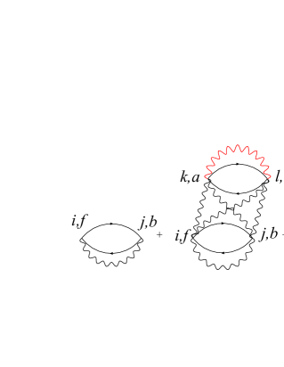
Figure 4: Diagrammatic series for the tunneling current corresponding to the real-time instanton configuration (LABEL:eq:Phi_Inst). Black wavy lines, representing the exponent of the phase correlation function, $\exp\{-J(\xi)\}$, are taken into account by the saddle-point approximation, while the red ones originate from the quantum fluctuations around the instanton.

Following this procedure, we find for the tunneling action in the saddle-point approximation

$$i\mathcal{A}^{*,<}_{t,ij} = \sum_{kl}\tau_{k}\tau_{l}\int_{{\cal C}_{K}}dt^{\prime}_{1,2}e^{i\Theta_{k}^{*}(t_{1}^{\prime})}\tilde{\Pi}_{kl}(t^{\prime}_{1},t^{\prime}_{2})e^{-i\Theta_{l}^{*}(t^{\prime}_{2})}.$$

with the phases

$$i\Theta_{k}^{*,a}(t) = J^{fa}(x_{i}^{+}-x_{k}^{+},t_{1}-t)-J^{ba}(x_{j}^{+}-x_{k}^{+},t_{2}-t)$$

$$+ J^{fa}(x_{i}^{-}-x_{k}^{-},t_{1}-t)-J^{ba}(x_{j}^{-}-x_{k}^{-},t_{2}-t)$$

($a$ is the Keldysh index). In the stationary situation this action should become a function of time difference only, $\mathcal{A}^{*,<}_{t,ij}(t_{1}-t_{2})$. We have also taken into account quantum fluctuations around the instanton trajectory $\varphi^{\alpha}_{*}$. One can prove that, in analogy with Ref. NgoDinh10, , they result in renormalization of the bare polarization operator $\Pi_{kl}$ to the dressed one given by

$$\tilde{\Pi}^{aa^{\prime}}_{kl}(t_{1},t_{2}) = {\Pi}^{aa^{\prime}}_{kl}(t_{1},t_{2})$$ (58)

$$\times \exp\{-J^{aa^{\prime}}(t_{1}-t_{2},x^{+}_{k}-x^{-}_{l})\}$$

$$\times \exp\{-J^{a^{\prime}a}(t_{2}-t_{1},x^{-}_{l}-x^{-}_{k})\}.$$

The tunneling current can be now evaluated by substituting the stationary phase $\Theta^{*}$ into relations (II.3) and (52). The diagrammatic representation resulting from expansion of the exponential of the tunneling action evaluated in the saddle-point approximation is shown in Fig. 4. If we retain only the first term of this expansion (i.e. neglect the tunneling action), we reproduce the result (II.3) of the previous section. The non-Gaussian shot noise modifies this result by the additional factor $e^{i\mathcal{A}_{t}^{*}}$ under the time integral,

$$I_{ij}^{\gtrless} = e\tau_{i}\tau_{j}v^{2}\int dt^{\prime}\exp\{iA_{t,ij}^{*,\gtrless}(t^{\prime})\}$$

$$\times G^{+,\gtrless}(x_{i}^{+}-x_{j}^{+},t^{\prime})G^{-,\lessgtr}(x_{j}^{-}-x_{i}^{-},-t^{\prime}).$$

The full Green’s function $G^{+}$ here contains the extra phase shift, which takes into account the non-equilibrium charge effects. It has to be found in accordance with Eqs. (II.1) and (16). Solving mean field equations (II.1) in the dc limit, i.e. at $\omega=0$, $q\sim 1/L$, with the use of $\rho_{0}=eV/(2\pi v)$ as the injected non-equilibrium charge, one gets the mean electrostatic potential on the upper arm of the interferometer,

$$\bar{\varphi}_{c}^{+}=\nu^{-1}\left(1-\frac{v}{u_{P}(1/L)}\right)eV$$ (60)

and the non-equilibrium phase shift

$$\bar{\Theta}_{c}^{+}(x)=\nu^{-1}\left(\frac{1}{u_{P}(1/L)}-\frac{1}{v}\right)eVx.$$ (61)

Using the expression (II.4), we can now derive a general result for the differential conductance ${\cal G}(V)=dI/dV$. Specifically, the conductance is obtained as a sum of two contributions: ${\cal G}_{0}(V)$ which is independent on the enclosed flux $\Phi$ and another one, ${\cal G}_{\Phi}(V)$, which is sensitive to $\Phi$,

$$\mathcal{G}(V)=\frac{e^{2}}{2\pi\hbar}\Bigl{(}\tau_{1}^{2}\mathcal{I}_{1}+\tau_{2}^{2}\mathcal{I}_{2}+2\tau_{1}\tau_{2}{\rm Re}\left(\mathcal{I}_{\Phi}e^{i\Phi}\right)\Bigr{)}\,,$$ (62)

where

$$\mathcal{I}_{k} \simeq 4\pi v^{2}\int dt\,te^{-ieVt}\mathrm{Im}(G_{0}^{>}(0,t))^{2}\exp\left\{-{\rm Im}\,A_{t,kk}^{*}(t)\right\}\,,$$

$$\mathcal{I}_{\Phi} \simeq 4\pi v^{2}\int dt(t-\Delta t)\,e^{-ieV(t-\Delta t)}\exp\{-{\rm Im}\,A_{t,12}^{*}(t)\}$$ (63)

$$\times \mathrm{Im}(G_{0}^{>}(l^{+},t)G_{0}^{<}(-l^{-},-t)).$$

In this expression $l^{\pm}=x_{2}^{\pm}-x_{1}^{\pm}$ are the lengths of the upper and lower arms of the MZI, and

$$\Delta t=\frac{\partial}{\partial(eV)}\Bigl{[}\,\bar{\Theta}^{+}_{c}(x_{2}^{+})-\bar{\Theta}^{+}_{c}(x_{1}^{+})\Bigr{]}+{l^{+}}/{v}$$ (64)

is the delay time related to the charging effects discussed in Sec. II.1. The explicit form of the delay time $\Delta t$ depends on specific model of the interaction. When deriving the result (63), we have neglected the real part of the tunneling action, ${\rm Re}\,A_{t}^{*}$ (it leads to small corrections only that do not affect the result in any essential way).

III Short-range interaction

In this section we analyze a model of an interferometer with $\nu=2$ channels per interferometer arm and short-range (point-like) interaction, $U_{0}(x-x^{\prime})=U_{0}\delta(x-x^{\prime})$. This model was considered previously in Ref. Levkivskyi08, where non-equilibrium dephasing effects were discarded. We will show that predictions of this model can not be reconciled with the experiments, which can be traced back to the simplified treatment of the interaction. Nevertheless, it is natural to start our analysis from this model that serves nicely for illustration of general principles.

The elementary excitations induced by the short-range interaction interaction are dispersiveness collective charge and neutral modes with velocities $u=v_{F}+{U_{0}}/{\pi}$ and $v$ respectively. The correlation functions read

$$J^{\gtrless}(x,t)=\frac{1}{2}\ln\left(\frac{x-ut_{\mp}}{x-vt_{\mp}}\right),$$ (65)

$$J^{T/\tilde{T}}(x,t)=\theta(t)J^{\gtrless}(x,t)+\theta(-t)J^{\lessgtr}(x,t),$$ (66)

where $t_{\pm}=t\pm i0$. It is easy to verify that Eq. (65) can be also written as

$$J^{T/\tilde{T}}(x,t)=\theta(x)J^{\gtrless}(x,t)+\theta(-x)J^{\lessgtr}(x,t)\,.$$ (67)

The last equation is a consequence of the chirality of the system. Similar relations hold also for the polarization operators $\Pi_{kl}$, and these relations remain unchanged after renormalization.

Using the relations (67) for the correlation functions, one can show that the saddle-point phase $\Theta^{*,a}_{k}$ does not depend on the Keldysh index $a$ if $k=2$. (We remind that, according to our convention, $x_{2}^{\pm}>x_{1}^{\pm}$.) Analogously, the renormalized polarization operator $\tilde{\Pi}^{aa^{\prime}}_{kl}$ does not depend on $a$ ($a^{\prime}$), if $k=2$ ($l=2$). Using the above relations and taking into account contributions from the forward and backward Keldysh contour, we find that the only non-vanishing term in the sum (II.4) for the tunneling action $\mathcal{A}_{t}^{*}$ is the one with $k=l=1$. In other words, the tunneling action in the saddle-point approximation has the only contribution $\propto\tau_{1}^{2}$, which means that only the noise produced by the first contact contributes to dephasing. This remarkable property has a simple physical explanation: in chiral 1D-system particles possess a well-defined prehistory, where the direction in space is linked to the direction of time. At zero temperature but finite voltage the tunneling of electrons via the first QPC is accompanied by a spontaneous emission of non-equilibrium plasmons and neutral modes. They transfer the shot noise $\propto\tau_{1}^{2}$ to the second QPC, where it affects the direct ($I_{22}$) and interference ($I_{12}$) current. On the other hand, the shot noise generated at the second QPC is transferred directly to the drains without affecting the particle interference.

Let us evaluate the tunneling action for the interference current $I_{12}^{<}$,

$$i\mathcal{A}_{t,12}^{*}=\tau_{1}^{2}\int dt^{\prime}_{1,2}e^{i\Theta_{1}^{*}(t^{\prime}_{1})}\tilde{\Pi}_{11}(t^{\prime}_{1}-t^{\prime}_{2})e^{-i\Theta_{1}^{*}(t^{\prime}_{2})},$$ (68)

$$e^{i\Theta_{1}^{*f/b}(t)}=\frac{(t+\frac{l^{+}}{v}\pm i0)^{\frac{1}{2}}(t+\frac{l^{-}}{v}\pm i0)^{\frac{1}{2}}}{(t+\frac{l^{+}}{u}\pm i0)^{\frac{1}{2}}(t+\frac{l^{-}}{u}\pm i0)^{\frac{1}{2}}},$$ (69)

where $l^{\pm}=x_{2}^{\pm}-x_{1}^{\pm}$ are the lengths of the interferometer arms. Remarkably, this action for the interference current does not depend on the times $t_{1,2}$, and therefore, the current factorizes in the one found in Sec. II.3 and a dephasing factor. The dominant large-voltage behavior of (68) is determined by the singularities of the polarization operator at $t^{\prime}_{1}\sim t^{\prime}_{2}\sim 1/eV$, yielding

$$i\mathcal{A}_{t,12}^{*}=-\tau_{1}^{2}\int_{-\infty}^{\infty}dt[\tilde{P}_{11}^{>}(e^{i\Theta_{1}^{*b}(t)-i\Theta_{1}^{*f}(t)}-1)$$

$$+\tilde{P}_{11}^{<}(e^{i\Theta_{1}^{*f}(t)-i\Theta_{1}^{*b}(t)}-1)],$$ (70)

where

$$\tilde{P}_{11}^{\gtrless}=\int dt\tilde{\Pi}_{11}^{\gtrless}(t)=-\frac{v}{u}\theta(\mp eV)\frac{|eV|}{2\pi}.$$ (71)

Thus, for the imaginary part of the action we have

$$\mathrm{Im}\,\mathcal{A}_{t,12}^{*}= - 2\tau_{1}^{2}[\tilde{P}_{11}^{>}+\tilde{P}_{11}^{<}]$$

$$\times \int_{-\infty}^{\infty}dt\sin^{2}\left(\frac{\Theta_{1}^{*b}(t)-\Theta_{1}^{*f}(t)}{2}\right).$$

The only effect of quantum corrections to the saddle-point approximation is a renormalization of the tunneling strength, $\tau_{1}^{2}\rightarrow\tilde{\tau}_{1}^{2}=\tau_{1}^{2}v/u$.

The final result for the dephasing rate depends on relation between the parameters of the problem. In the case $l^{+}/l^{-}>u/v$, we find

$$\mathrm{Im}\,\mathcal{A}_{t,12}^{*}=\tilde{\tau}_{1}^{2}\frac{1}{\pi}|eV|(l^{+}+l^{-})\left(\frac{1}{v}-\frac{1}{u}\right).$$ (73)

Therefore, in this regime the dephasing rate is proportional to the total length of the interferometer. Clearly, there is no dephasing when the velocities are equal to each other, which is the case for the non-interacting system. If parameters are chosen in such a way that $l^{+}/l^{-}<u/v$, we get

$$\mathrm{Im}\mathcal{A}_{t,12}^{*}=\tilde{\tau}_{1}^{2}\frac{1}{\pi}|eV||l^{+}-l^{-}|\left(\frac{1}{v}+\frac{1}{u}\right).$$ (74)

Remarkably, we find no dephasing in the case of equal arm lengths. We offer the following physical interpretation of this result. A tunneling event at the first contact is accompanied by emission of plasmons in the upper and lower interferometer arms. If the arm lengths are equal, the plasmons meet together at the second contact completely phase-coherently. In other words, when electrons tunnel at the first contact, there will be noise created in the upper and lower interferometer arm, and this noise is fully correlated. In the case of equal arm lengths it is possible to restore the complete phase information at the second contact. Thus, dephasing is absent.

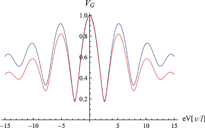
Figure 5: Visibility at $\nu=2$ calculated in the model of strong short-range interaction, $u\gg v$, with equal QPCs, $\tilde{\tau}_{1}^{2}=0.2$. Blue curve: dephasing is neglected; red curve: dephasing by the shot-noise is taken into account. Upper panel: $l^{+}/l^{-}=1.15$; lower panel: $l^{+}/l^{-}=1.35$.

In the case of direct currents, an analogous calculation for the long-time limit gives

$$\mathrm{Im}\,\mathcal{A}_{t,11}^{*}(t) = 0,$$ (75)

$$\mathrm{Im}\,\mathcal{A}_{t,22}^{*}(t) = \tilde{\tau}_{1}^{2}\frac{4}{\pi}|eVt|.$$

As for the time delay $\Delta t$ related to the charging of the upper arm of the interferometer, we obtain, using Eqs. (II.1), (16) and (64),

$$\Delta t=\frac{l^{+}}{2}\left(\frac{1}{u}+\frac{1}{v}\right).$$ (76)

We now have all the ingredients needed to evaluate the visibility of the MZI according to Eqs. (62) and (63) for the differential conductance. We define the voltage dependent visibility as the ratio of the amplitude of Aharonov-Bohm oscillations in conductance to its mean value:

$${\cal V}_{G}(V)=\Bigl{(}\max({\cal G}_{\Phi}(V))-\min({\cal G}_{\Phi}(V))\Bigr{)}/2\,{\cal G}_{0}(V).$$ (77)

We observe that the direct conductance ${\cal G}_{0}(V)$ does not depend on voltage despite a non-zero action $A^{*}_{t,22}$: the latter affects each of the tunneling rates $I^{>}_{22}$ and $I^{<}_{22}$ but does not change their difference. Therefore, the visibility can be expressed via the integral ${\cal I}_{\Phi}$ given by the relation (63) as

$${\cal V}_{G}(V)=\frac{2\tau_{1}\tau_{2}}{\tau_{1}^{2}+\tau_{2}^{2}}|{\cal I}_{\Phi}|\,.$$ (78)

In what follows we consider the limit of strong interaction, $u\gg v$. In this case we represent ${\cal I}_{\Phi}$ in the form

$${\cal I}_{\Phi}={\cal I}_{\Phi}^{(0)}\exp\{-{\rm Im}\,{\cal A}^{*}_{t,12}\},$$ (79)

where ${\cal I}_{\Phi}^{(0)}$ is simplified to

$$\mathcal{I}_{\Phi}^{(0)}= - \int\frac{dt}{\pi}(t-\Delta t)e^{-ieV(t-\Delta t)}$$

$$\times {\rm Im}\left[\frac{1}{(t+i0)(t-\frac{\Delta x^{+}}{v}+i0)^{\frac{1}{2}}(t-\frac{\Delta x^{-}}{v}+i0)^{\frac{1}{2}}}\right]\,.$$

Two examples of the visibility plots in the strong-interaction limit and equal transmissions at both QPCs are shown in Fig. 5, where we have denoted $l=(l^{+}+l^{-})/2$.

While the obtained voltage dependences of visibility does show an oscillatory structure similar to experimentally observed lobes, there are strong differences. Most importantly, in the limit of equal arms, which is predominantly the experimental situation, the visibility calculated in the framework of short-range interaction model oscillates as ${\cal V}_{G}\propto\cos(eVl/v)$ without any decay, since the non-equilibrium dephasing rate vanishes according to the relation (74) whatever strong the interaction is. The situation gets even worse when we try to apply the same model to describe experimental data on MZI at $\nu=1$. Specifically, the model predicts then a constant visibility, which is in stark contrast to the experiments that show lobe structures for $\nu=1$ as well.

To summarize, the Keldysh action approach allows us to determine the tunneling current through the MZI. The theory includes all the effects of the interaction, including charging, renormalization, and dephasing. The dephasing rate grows linearly with voltage; the source of dephasing is the shot noise produced at the first QPC. The calculation of this section were carried out under the assumption of short-range interaction (which would be the case for a system with a nearby metallic gate). Essential discrepancies between the theoretical findings for this model and the experimental data indicate the importance of long-range ($1/r$) character of the Coulomb interaction. The corresponding model will be studied in the next section.

IV Long-range interaction

In this section, we consider the model of the MZI with the long-range Coulomb interaction,

$$U_{0}(x)=\frac{e^{2}}{\epsilon}\frac{1}{\sqrt{x^{2}+b^{2}}},$$ (81)

which is regularized at short distances by the finite width of the edge state $b$. Using the self-consistent electrostatic picture Chklovskii92 of the quantum Hall edge channels in the smooth confining potential, we associate the scale $b$ with the typical width of a compressible strip. The latter satisfies

$$b\gg a\sim l_{B},$$ (82)

where $a$ is the short distance cut-off introduced earlier (see also estimates of typical experimental parameters in Sec. IV.3). The strength of Coulomb interaction is quantified by the dimensionless coupling constant

$$\alpha=\frac{\nu\,e^{2}}{\epsilon\,\pi v},$$ (83)

where $\epsilon$ is the dielectric constant. As discussed below in Sec. IV.3, the edge velocity $v$ (which is also the velocity of the neutral mode at filling factor $\nu=2$) is fixed within the self-consistent electrostatic picture in such a way that $\alpha\sim 1$. In the momentum space

$$U_{0}(q)=\frac{2e^{2}}{\epsilon}K_{0}(|q|b),$$ (84)

with the small-$q$ asymptotic behavior

$$U_{0}(q)\simeq-\frac{2e^{2}}{\epsilon}\ln(|q|bd),\quad q\ll b^{-1},$$ (85)

where $K_{0}$ is the modified Bessel function of the second kind and the numerical constant $d=e^{\gamma_{E}}/2=0.89$.

IV.1 Plasmon correlation function

Consider now the plasmon phase correlation function (22). It is given by

$$J^{>}_{P}(x,t)=\int_{0}^{\infty}\frac{dq}{q}\Bigr{(}1-e^{i\phi(q)}\Bigl{)}e^{-aq},$$ (86)

where we have introduced the phase $\phi(q)$, containing the $x$- and $t$-dependence,

$$\phi(q) = qx-\omega_{P}(q)\,t,$$ (87)

$$\omega_{P}(q) = vq\,(1+{\alpha}\,K_{0}(|q|b)).$$ (88)

As follows from the integral representation (86), at zero temperature $J^{>}_{P}(x,t)$ is an analytic function of time in the upper half-plane. We now analyze this function in the relevant parameter limit

$$\max\{t,x/v\}\gg b/v\gg a/v.$$ (89)

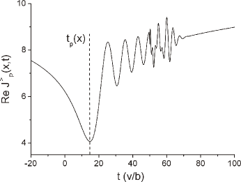
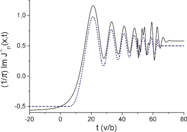
Figure 6: Real (upper panel) and imaginary(lower panel) parts of the plasmon correlation function plotted versus the dimensionless time at fixed $x/b=50.0$; the coupling constant $\alpha=1.0$ and $a/b=0.1$. The dashed line shows the analytical approximation (97).

The time dependence of real and imaginary parts of the phase correlation function $J^{>}_{P}(x,t)$ for typical values of parameters is shown in Fig. 6. One observes characteristic oscillations which stem from the non-linear plasmon dispersion $\omega_{P}(q)=u_{p}(q)q$ given by Eq. (88). As a result, the initially localized density wave packet injected into the interferometer arm at some position $x^{\prime}=0$ and time $t^{\prime}=0$ is spread after some time $t$, when it arrives at given point $x$. This is because its constituents — bosonic modes, with different wave vectors $q$ — propagate with different group velocities. The real part of the phase correlation function has a pronounced minimum at

$$t_{p}(x)=\frac{x}{u_{p}(q)}\Biggl{|}_{q\sim 1/x}\simeq\frac{x}{\alpha\,v\ln\left(e\,x/b\tilde{d}\right)},$$ (90)

where we have introduced

$$\tilde{d}(\alpha)=de^{(\alpha-1)/\alpha},$$ (91)

and the numerical constant $d$ has been defined below Eq. (84). The time $t_{p}(x)$ is a typical time scale required for the fastest plasmon (that has the smallest possible momentum $q\sim 1/x$) to traverse the distance $x$. The plots at Fig. 6 should be contrasted with the behavior of $J^{>}_{P}(x,t)$ in the short-range interaction model given by Eq. (65). In the latter case the real part of $J^{>}_{P}(x,t)$ is a smooth function with logarithmic singularity at $t=x/v$, while the imaginary part is piecewise constant.

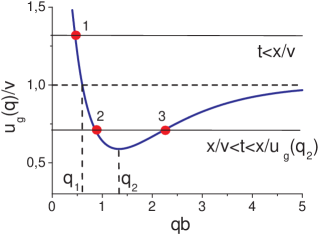
Figure 7: The group velocity of plasmons shown as function of the dimensionless momentum for the coupling constant $\alpha=2$. At $q_{1}b=0.59$ one has $u_{g}(q_{1})=v$ and for $q_{2}b=1.33$ the group velocity is at minimum.

The oscillatory behavior of $J_{P}^{>}(x,t)$ can be qualitatively understood using the stationary phase approximation to the integral (86). For technical details of this analysis we refer the reader to Appendix D. The saddle point $q_{*}(x,t)$ of the phase $\phi(q)$ for given $x$ and $t$ can be found numerically as the solution of the equation

$$x=u_{g}(q_{*})t,$$ (92)

where we introduced the group velocity

$$u_{g}(q) = \frac{\partial\omega_{P}(q)}{\partial q}$$

$$= v\Bigl{(}1+\alpha\,K_{0}(qb)-\alpha\,(qb)K_{1}(qb)\Bigr{)}$$

of the plasmon mode. The plot of the function $u_{g}(q)$ is presented in Fig. 7. As one can see, there are two special momenta, $q_{1}$ and $q_{2}$, both being independent on coupling strength $\alpha$. At $q=q_{1}$ the group velocity matches the drift velocity $u_{g}(q)=v$, while at $q=q_{2}$ the group velocity reaches its minimum. Thus, for given $x$ and at $t<x/v$ the stationary phase equation (92) has a single root (see Fig. 7). In the short-time limit one finds asymptotically

$$q_{*}(x,t) \simeq \left(b\tilde{d}\right)^{-1}e^{-x/\alpha\,vt},$$ (94)

$$\phi(q_{*}) \simeq -\alpha\,q_{*}v\,t,\qquad t\ll x/v.$$

The unique saddle point leads to approximately single-period oscillations in the phase correlation function at

$$t_{p}(x)\lesssim t<x/v,$$ (95)

as is indeed seen in the numerical plots in Fig. 6. We also remark that at $t\sim t_{p}(x)$ the optimal phase $\phi(q_{*})$ becomes of order unity, thus the stationary phase method loses its applicability. At still smaller times the integral (86) is governed by the contribution of the end point at $q=0$ and shows no oscillations. On the other hand, in the time interval

$$x/v<t<x/u_{g}(q_{2})$$ (96)

one finds (see Fig. 7) two distinct roots of the stationary phase equation (92). In this range the plasmon phase correlation functions acquires characteristic beatings arising from the interference of the two contributions (with generally incommensurable phases) corresponding to two stationary-point momenta.

It is shown in Appendix D that at $t<u_{g}(q_{2})$ the imaginary part of the phase correlation function can be approximated in the following way:

$${\rm Im}\,J_{P}^{>}(x,t)=\pi/2-\sqrt{2}\pi{\rm Re}\left[\,{\rm Erfc}\sqrt{-i(\phi_{*}-\phi_{0})}\,\right],$$ (97)

where $\phi_{*}=\phi(q_{*}(x,t))$ is the stationary phase, ${\rm Erfc}(z)$ is the complementary error function, and the constant $\phi_{0}$ is defined as the root of the equation ${\rm Re}\left[{\rm Erfc}\sqrt{i\phi_{0}}\right]=1/\sqrt{2}$. The above approximation is shown by the dotted line in Fig. 6; one finds a good agreement with the exact numerical curve. We will use this approximation later to evaluate the dephasing action with the logarithmic accuracy.

IV.2 Visibility

Let us turn now to the analysis of the visibility. For that purpose we have to find the differential conductance in accordance with general relations (62) and (63) of Sec. II. We will first perform the analysis in the framework of the Gaussian approximation (Sec. II.3), i.e. neglecting the tunneling action ${\rm Im}\,A^{*}_{t}$ in Eq. (63). Later we will include the effects of the non-Gaussian fluctuations.

IV.2.1 Filling factor $\nu=1$

In the case $\nu=1$ the Green function $G_{0}$ at zero bias is determined solely by the plasmon part of the total correlation function $J(\xi)$, since the free part $J_{F}(\xi)$ cancels against the bare Green function $g_{0}$:

$$G_{0}^{>}(x,t)=\frac{1}{2\pi i\,a}e^{-J^{>}_{P}(x,t)}.$$ (98)

The “lesser” Green function satisfies $G_{0}^{<}(x,t)=\left(G_{0}^{>}(x,t)\right)^{*}$. In the case of finite voltage the above expression for the upper arm is modified to

$$G_{+}^{\gtrless}(x,t)=\exp\left\{-ieV\left(t-\frac{x}{u_{P}(1/L)}\right)\right\}G_{0}^{\gtrless}(x,t),$$ (99)

where we took into account the non-equilibrium phase shift (61).

In the following we concentrate on the case of symmetric interferometer, $l^{+}=l^{-}\equiv l$. We will show that, in contrast to the results of Sec. III, even in this situation the visibility is a non-trivial function of voltage. A small mismatch in the lengths of upper and lower arms will not affect our conclusions essentially.

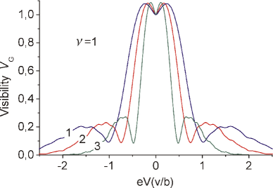
Figure 8: Visibility of Aharonov-Bohm oscillations in a symmetric Mach-Zehnder interferometer at $\nu=1$ calculated in the model of long-range Coulomb interaction with the coupling constant $\alpha=1$, shown for $a/b=0.1$ and different ratios of $l/b$: (1)-30; (2)-50; (3)-100.

In the Gaussian approximation the visibility of interference oscillations can be found by integrating Eq. (63) over the time numerically. As discussed above, we neglect the dephasing caused by the shot noise at this stage and will restore it later. Using Eqs. (64), we obtain for the delay time

$$\Delta t\,=\,\frac{l}{u_{P}(1/L)}\,\simeq\,t_{p}(l)\,.$$ (100)

In a typical experimental layout the distance from source to drain $L$ is of the order of MZI size $l$. Thus, within the logarithmic accuracy (i.e. up to a numerical factor in the argument of the logarithm) the delay time is actually equal to the scale $t_{p}(l)$ defined by Eq. (90).

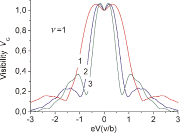
Figure 9: Visibility of Aharonov-Bohm oscillations in a symmetric MZI at $\nu=1$ calculated in the model of long-range Coulomb interaction for different coupling constant $\alpha$: (1)-2.0; (2)-1.0; (3)-0.5. The other parameters are: $l/b=30$ and $a/b=0.1$.

The visibility ${\cal V}_{G}$ calculated in accordance with the definition (77) is shown in Fig. 8 for different values of the ratio $l/b$ and in Fig. 9 for different values of the coupling constant $\alpha$. In all cases the MZI is symmetric, meaning that $l^{+}=l^{-}$ and both QPCs are equivalent. The plots clearly show a non-trivial voltage dependence of visibility, with three lobes. The width $\epsilon_{0}$ of the central peak scales as

$$\epsilon_{0}\sim 2\pi/t_{p}(l)\sim 2\pi\alpha\frac{v}{l}\ln(l/b)$$ (101)

A dip in the visibility at small voltage is the result of a zero-bias anomaly in the direct ${\cal G}_{0}(V)$ and interference ${\cal G}_{\Phi}(V)$ part of conductance.

As has been already emphasized, the appearance of the lobe structure in visibility in the model of long-range Coulomb interaction at $\nu=1$ crucially depends on non-linearity of plasmon dispersion, which gives rise to the oscillatory behavior of the phase correlator $J_{P}(x,t)$ as the function of time. We also note that additional weak oscillations in ${\cal V}_{G}$ (seen on top of the lobe pattern) stem from the beating in the plasmon correlation function in the time interval (96), which is due to plasmons with short momenta $q\sim b^{-1}$.

Our calculations in this subsection are closely related to those of Ref. Chalker07, where the effect of non-linearity of plasmon dispersion on properties of a $\nu=1$ MZI was analyzed. The crucial difference is that we also take into account the phase shift (61) representing a non-equilibrium charging effect. For this reason, our non-equilibrium Green function (99) and the resulting visibility ${\cal V}_{G}$ differ from their counterparts in the work Chalker07, . The voltage dependence of visibility shown in Figs. 8 and 9 results from a combined effect of non-linear dispersion and charging.

IV.2.2 Filling factor $\nu=2$

We have carried out analogous calculations for the setup with $\nu=2$. As before, we concentrate on the symmetric MZI. In the case of two edge states per interferometer arm a tunneled electron excites plasmon and neutral modes. The electron propagator at zero voltage acquires the form

$$G_{0}^{>}(x,t)=\frac{1}{2\pi\sqrt{iav}}\frac{e^{-J^{>}_{P}(x,t)/2}}{\sqrt{x/v-t+ia/v}}\,.$$ (102)

The delay time for the setup of Fig. 1 with one of outer channels biased can be found using Eq. (64),

$$\Delta t\simeq\frac{l}{2}\left(\frac{1}{u_{P}(1/l)}+\frac{1}{v}\right)\,.$$ (103)

It is instructive to compare this result with Eq. (100): one sees a clear manifestation of two modes (plasmon and neutral) for $\nu=2$ instead of a single plasmon mode at $\nu=1$. The voltage dependence of visibility calculated numerically in the Gaussian approximation is shown by the upper curve in Fig. 10. (The lower curve in the same plot is the visibility calculated in the instanton approximation, which takes into account the extra dephasing due to the non-equilibrium shot-noise, Sec. IV.2.3.) One can see that the voltage dependence of visibility is qualitatively different from the $\nu=1$ setup. Specifically, the visibility ${\cal V}_{G}(V)$ shows many oscillations (“lobes”) as the function of bias with a typical width given by the Thouless energy of the MZI,

$$\epsilon_{\rm Th}=\pi v/l\,.$$ (104)

This energy scale differs from the characteristic scale $\epsilon_{0}$ characterizing lobes in the $\nu=1$ MZI [see Eq. (101)] by a logarithmic factor.

The results of this subsection should be also contrasted with those of Sec. III. The visibility ${\cal V}_{G}(V)$ calculated there for the same setup ($\nu=2$) but in the model of short-range interaction demonstrates the $\cos$-like oscillations which, however, do not decay in the case of a symmetric MZI. In the $1/r$ model of Coulomb interaction considered here, the visibility ${\cal V}_{G}(V)$ oscillations do decay already in the Gaussian approximation, as seen in Fig. 10. Furthermore, as we are going to show in Sec. IV.2.3, the shot-noise dephasing leads in this case to an additional suppression of oscillations of visibility and to a decay of visibility down to zero at high voltage (rather than to a constant as in the Gaussian model).

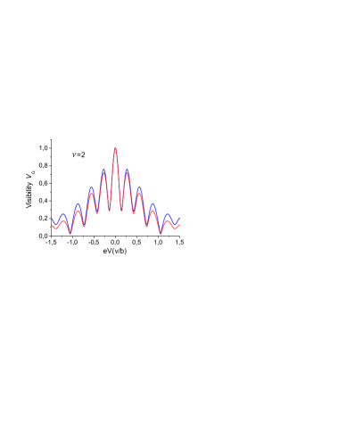
Figure 10: Visibility of Aharonov-Bohm oscillations in a symmetric MZI at $\nu=2$ calculated in the model of long-range Coulomb interaction with the coupling constant $\alpha=1$, shown for $l/b=30$ and $a/b=0.1$. Upper curve: Gaussian approximation; lower curve: shot-noise dephasing with $\tau_{1}^{2}=0.2$ is taken into account.

IV.2.3 Non-equilibrium dephasing by the shot noise

Let us now calculate the suppression of the visibility due to non-Gaussian phase fluctuations following the method of Sec. II.4.

In the instanton approximation the optimal phases $\Theta^{*,a}_{k}$ are expressed in terms of the phase correlation function $J(x,t)$ according to Eq. (LABEL:eq:Phi_Inst). We saw in section III that the special properties (67) of the causal correlators $J^{T/\tilde{T}}(x,t)$ in the case of short-range interaction greatly simplify the calculations. The question arises whether these properties are also valid in the case of long-range interaction. Since $J^{>}(x,t)=\left(J^{<}(x,t)\right)^{*}$, we conclude that $J^{>}$ and $J^{<}$ may differ only in the imaginary part. As is clearly seen in Fig. 6, at $x>0$ and $t<0$ (or, at $x<0$ and $t>0$) we have ${\rm Im}J^{>}_{P}\simeq{\rm Im}J^{>}_{F}=-\pi/2$, so that the imaginary part of the full correlator, ${\rm Im}J^{>}$, in the same range of parameters is almost zero. It follows that the relations (67) are approximately satisfied. This is a manifestation of the fact that even in the presence of spectral dispersion the edge modes retain their chiral character.

Performing calculation similar to those in Sec. III, we arrive again at the result (III), which can be cast in the form

$$\mathrm{Im}\,\mathcal{A}_{t,12}^{*}=2\tau_{1}^{2}\mathcal{P}(eV)\Upsilon(l),$$ (105)

where $\mathcal{P}(eV)$ is the noise power,

$$\mathcal{P}(eV)=-\int_{-\infty}^{\infty}dt\left(\tilde{\Pi}_{11}^{<}(t)+\tilde{\Pi}_{11}^{>}(t)\right),$$ (106)

and

$$\Upsilon(l)=\int_{0}^{+\infty}dt^{\prime}\sin^{2}\left(\frac{2}{\nu}\mathrm{Im}\,J^{>}_{\rm P}(l,t^{\prime})-\frac{\pi}{\nu}\right)$$ (107)

is a characteristic bosonic dwell time related to the size of the MZI. In what follows, we will find the dephasing action (105) with the logarithmic accuracy (up to a coefficient of order unity under the logarithm).

First, we evaluate the noise, using its representation in terms of interacting Green function

$$\mathcal{P}(eV)=4v^{2}\int_{-\infty}^{+\infty}dt\sin^{2}(eVt/2)\,{\rm Re}\left[G_{0}^{>}(0,t)\right]^{2}.$$ (108)

To derive this expression, we have used the relation $G_{0}^{<}(0,t)=\left(G_{0}^{>}(0,t)\right)^{*}$ and the fact that at zero temperature and at $eV\to 0$ the shot noise should vanish. To find the interacting Green function, we evaluate the momentum integral (86). At large times $t\gg b/v$ it is given by

$$J^{>}_{P}(t)\simeq\ln(1/q^{*})+{\rm const}\,.$$ (109)

Here the momentum $q^{*}$ satisfies the condition $|\phi(q^{*})|\sim 1$, which at $x=0$ leads to

$$(q^{*})^{-1}\simeq\alpha vt\ln\left({evt}/{b\,\tilde{d}}\right)$$ (110)

(here $e$ stands for the base of natural logarithms rather than for the electron charge). On the other hand, at small times $t\ll b/v$ the plasmon correlator is determined by the large-momentum behavior of the integrand in Eq. (86), where interaction is absent and thus $J^{>}_{P}(t)$ should coincide with the free result. An approximation for the interacting Green function which respects both limits is given by

$$G^{>}_{0}(0,t)\sim\frac{1}{2\pi\alpha^{1/\nu}(vt-ia)\ln^{1/\nu}\left(e+ievt/b\,\tilde{d}\right)},$$ (111)

where we have also taken into account that $G^{>}_{0}(0,t)$ must be analytic in the upper half plane of complex $t$. The main contribution to the integral in Eq. (108) comes from times $t\sim 1/eV$. Evaluating the integral, we finally find

$$\mathcal{P}(eV)\sim\frac{|eV|}{2\pi\alpha^{2/\nu}\ln^{2/\nu}\Bigl{(}e+\,v/|eV|b\,\tilde{d}\Bigr{)}}.$$ (112)

Note that the noise power reveals a weak zero-bias anomaly in the chiral 1D system, which originates from the long-range nature of the Coulomb interaction.

Let us now evaluate the bosonic dwell time (107). One can employ the saddle point approximation (97) and change the integration variable from time $t^{\prime}$ to phase $\phi$ using the relation (94). We find with the logarithmic accuracy

$$t\simeq\frac{l}{\alpha\,v}\left[\ln\left(\frac{l}{b\,\phi\,\tilde{d}}\right)\right]^{-1}\,.$$ (113)

This enables us to cast the dwell time (107) into the form

$$\Upsilon(l) \simeq \frac{l}{\alpha v}\int_{0}^{\phi_{\max}}\frac{d\phi}{\phi}\ln^{-2}\left(\frac{l}{b\,\phi\,\tilde{d}}\right)$$ (114)

$$\times \sin^{2}\left[\frac{2\pi\sqrt{2}}{\nu}\mathrm{Re}\left({\rm Erfc}\sqrt{i(\phi_{0}+\phi)}\right)\right],$$

where $\phi_{\max}\sim\alpha(l/b)/e$. This upper limit of integration originates from the fact that the integral in Eq. (107) is actually limited to times $t\lesssim l/v$. Let us now assume that the interaction is not too weak, so that $\phi_{\max}\gg 1$. This is always the case in the experiment, as will be shown in Sec. IV.3. Since the integral (114) converges at large $\phi$ (and is dominated by $\phi\sim 1$), one can now extend the integration up to infinity and also neglect the weak logarithmic dependence on the phase $\phi$. In this way we find

$$\Upsilon(l)\simeq C_{\nu}\left(\frac{l}{\alpha v}\right){\ln^{-2}\left(\frac{l}{b\,\tilde{d}}\right)},$$ (115)

where $C_{1}=3.96$ and $C_{2}=2.97$.

Equation (105) together with Eqs. (112) and (115) is the main result of this subsection. We see that the non-equilibrium dephasing action in the model of long-range Coulomb interaction is a sub-linear function of both the voltage and the size of the interferometer. Equation (105) tells us that the non-equilibrium dephasing in the MZI occurs due to the intrinsic shot noise. This noise is transferred by plasmons (in case of $\nu=1$) or by a superposition of plasmon and neutral bosonic modes (in case of $\nu=2$), which typically propagate through the MZI faster than electrons, as is seen from Eq. (115).

In Fig. 10 we illustrate the suppression of the visibility by the shot noise for the setup with $\nu=2$. The effect of shot-noise dephasing leads to suppression of visibility at high voltages. However, the lobe structure remains well preserved: the dephasing effect becomes strong only for voltages much larger than the period of the oscillations in visibility. The reason for this is twofold. First, this is a factor $\tau_{1}^{2}$ in Eq. (105) that was assumed to be small in our calculation. (We used the value $\tau_{1}^{2}=0.2$ in the plot.) We can expect a somewhat stronger dephasing due to the shot noise $\sim\tau_{1}^{2}(1-\tau_{1}^{2})$, when the QPC transparency is of order $50\%$. Second, there are logarithmic factors in Eqs. (112) and (115); their combined effect at the scale $eV\sim v/b$ and at $\nu=2$ leads to the suppression of the dephasing action by a factor $1/\ln^{3}(l/b)\ll 1$. Because of this factor, the lobe structure should not be destroyed by dephasing (i.e. many oscillations will be seen) even in the case of most noisy QPC with transparency of order $50\%$, in agreement with experiments.

A more detailed comparison of our findings with experiment is presented below.

IV.3 Comparison to experiment

Let us now discuss the relation of theoretical results of Sec. IV to experimental observations. The striking lobe-type structure in the visibility as function of voltage at low temperature was discovered for the first time in the experiment heiblum06 . At filling factor $\nu=1$ three lobes were reported, while at $\nu=2$ five lobes were observed. Later experiments of the same group with the use of somewhat different layout Ofek showed up to 9 lobes for $\nu=2$. The important part of the MZI setup in the experiment heiblum06 was an additional QPC0, which enabled to apply different chemical potentials to the outer and inner edge channels, see Fig. 1. These observations were corroborated by subsequent works roche07 ; strunk08 , where an analogous MZI layout with QPC0 was studied.

Our theoretical calculations carried out within the model of long-range Coulomb interaction (Sec. IV) compare well with the above experimental findings. On the qualitative level, we find three lobes in the case of $\nu=1$ (Figs. 8 and 9) and structure with many lobes for $\nu=2$ (Fig. 10), in agreement with the experiments.

Let us also note that a more complicated behavior of the finite-bias visibility was observed in another experimental work schoenenberger , where the MZI setup did not contain an additional QPC0. The emphasis of this study was on the asymmetry of the MZI characteristics when the transparency of the QPC1 was varied from 0 to 1. We cannot treat this feature within our approximation valid in the weak-tunneling regime.

More quantitative comparison of theoretical and experimental results requires the knowledge of the edge velocity $v$ and the range $b$ of the Coulomb interaction. To estimate them, we use the results of works Chklovskii92, ; Aleiner94, . In Ref. Aleiner94, the excitation spectrum of the compressible Hall liquid in the classical limit $\nu\gg 1$ was found. It consists of the magnetoplasmon mode with

$$\omega_{0}(q)=vq\ln\left(e^{-\gamma}/|q|\bar{l}\right),$$ (116)

and the acoustic spectrum with

$$\omega_{n}(q)=vq/n,\quad n\geq 1,$$ (117)

where $v$ is the drift velocity,

$$v=\frac{\nu e^{2}}{\epsilon\pi\hbar},$$ (118)

and $\bar{l}$ is the half of the width of the depletion layer between the confining gate and the 2DEG. The latter scale was found in Ref. Chklovskii92, and is controlled by the gate voltage,

$$\bar{l}\simeq\frac{V_{g}\epsilon}{4\pi n_{0}e}.$$ (119)

For the typical concentration $n_{0}\sim 2\times 10^{11}$cm^-2, the gate potential $V_{g}\sim$1V, and $\epsilon=12.5$, one thus gets an estimate $\bar{l}\sim 110\,$nm. This result is also believed to be applicable in the case of etched mesostructures, e.g. those used in the MZI setups. In this case the voltage $V_{g}$ should be associated with a work function, which for GaAs-AlGaAs heterostructures has the same energy scale $\sim 1$ eV.

In the quantum Hall regime, at $\nu=1$ and $\nu=2$, one expects that the above modes with $n=0,1$ should match the two chiral bosonic modes of our theory. We thus see that the drift velocity (118) would fix the interaction constant $\alpha$, defined by Eq. (83), to be of order 1. At the same time, comparing the dispersion relation (117) to Eqs. (84) and (88), we obtain the estimate for the scale $b$ in our theory, $b\simeq 2e^{\gamma}\bar{l}\sim 400\,$nm.

Let us first discuss the case $\nu=2$. For the typical size of the MZI, $l\sim 10\,\mu$m, one gets the ratio $l/b\sim 25$. This parameter controls the overall number of lobes in our theory, $N\sim l/\pi b$, cf. Fig.10. For sufficiently large transparency of QPCs the shot-noise dephasing will suppress the visibility at sufficiently large voltages corresponding to lobe indices $\gtrsim 1/\ln^{3}(l/b)$, see Sec. IV.2.3. However, for $l/b\sim 25$ this happens to be not so important for the lobe structure. To find the energy scale for the lobe structure, we estimate the drift velocity according to Eq. (118) that yields $v\sim 10^{5}$ m/s. This results in the following value of the Thouless energy  (104): $\epsilon_{\rm Th}\sim 20\,\mu$eV. This is indeed the typical energy scale seen in the above discussed experiments heiblum06 ; roche07 ; strunk08 .

We turn to the case of filling factor $\nu=1$. We obtain bias dependences of visibility with three lobes in a sufficiently broad range of parameters (see Figs. 8 and 9), in agreement with experimental works heiblum06 ; strunk08 . The energy scale for the lobes in our theory is given by Eq. (101), which is larger than the Thouless energy $\epsilon_{\rm Th}$ by a factor $\ln(l/b)$. For realistic values of parameters (see above), this factor is $\sim 3$. In the experiment the energy scales for $\nu=1$ and $\nu=2$ are practically equal. This discrepancy may be partly explained by the fact that, according to Eq. (118), the drift velocity is expected to be twice smaller for $\nu=1$ compared to $\nu=2$, which reduces the energy scale by factor of 2, partly compensating the logarithmic factor.

V Summary

In this paper we have discussed the influence of the Coulomb interaction on the quantum coherence in the electronic Mach-Zehnder interferometer (MZI) formed by integer quantum Hall edge states at filling fractions $\nu=1$ and $\nu=2$ out of equilibrium. Our main results can be summarized as follows.

1. We have developed the non-equilibrium functional bosonization framework which enables us to build up the Keldysh action of interacting electrons in the MZI. The most non-trivial term in the action is expressed in terms of a single-particle time-dependent interferometer scattering matrix in the dynamically fluctuating field and has a structure of a Fredholm determinant similar to those appearing in the theory of full counting statistics. We have used this action to analyze the limit of weak electron tunneling between interferometer arms in the case of arbitrarily strong e-e interaction. Our theory contains all interaction-induced effects on transport through MZI, including charging, dispersion non-linearity, and non-equilibrium decoherence.

2. Restricting at first the theoretical analysis to the Gaussian approximation for electron phase fluctuations, we have readily reproduced the previous theoretical results related to oscillations (lobe structure) in the dependence of the visibility on the bias voltage. Going beyond the Gaussian approximation, we have used a real-time instanton approach to evaluate the non-equilibrium dephasing rates that lead to further suppression of the Aharanov-Bohm oscillations in conductance with the increase of voltage. We have found that the out-of-equilibrium dephasing rate is proportional to the voltage dependent shot noise of the first quantum point contact (QPC1), defining the MZI, and originates from the emission of non-equilibrium plasmons and neutral bosonic modes in course of inelastic electron tunneling.

3. The results obtained within the model of short-range interaction (Sec. III) show strong contradictions to the experiment. Specifically, in the case of equal arms the visibility oscillations in the $\nu=2$ interferometer do not decay with voltage. For $\nu=1$ the problem is even more severe, as the visibility does not depend on the voltage at all.

4. Considering the realistic model of the long-range ($1/r$) Coulomb interaction, we are able to explain the experimentally observed dependence of the visibility of the interference signal at filling fraction $\nu=1$ and $\nu=2$. The origin of this effect is found to be a combination of three factors:

   • the electrostatic phase shift effect, related to the charge imbalance on different arms of the interferometer,

   • the interaction induced effect of the plasmon dispersion, and

   • the out-of-equilibrium decoherence due to the intrinsic shot noise.

   Using realistic parameters, we find three lobes in the bias dependence of visibility in the case of $\nu=1$ (Figs. 8 and 9) and structures with many lobes for $\nu=2$ (Fig. 10), in agreement with the experiments. The energy scale for the lobe structure in the visibility for $\nu=2$ is given by the Thouless energy of the MZI which is estimated as $\sim 20\,\mu$eV for realistic parameters, again in good agreement with experiment. For $\nu=1$ the energy scale for the lobes in our theory is enhanced by a factor $\ln(l/b)\simeq 3$, which is partly compensated by a difference in the drift velocity (and thus Thouless energy) at $\nu=1$ and $\nu=2$. There remains some discrepancy in this point with the experiment which indicates that the energy scales for $\nu=2$ and $\nu=1$ lobe structures are practically equal. This issue may be worth further study.

We anticipate that the approach developed in this work will be useful for a much broader class of electronic interference setups relevant to current or forthcoming experiments. The prospects for future research include, in particular, interferometers operating in the fractional quantum Hall regime as well as those built on edge states of topological insulators.

VI Acknowledgements

We thank Y. Gefen, I.V. Gornyi, M. Heiblum, I.P. Levkivskyi, S. Ngo Dinh, N. Ofek, and D.G. Polyakov for useful discussions. This work was supported by the German-Israeli Foundation Grant No. 965, by the EUROHORCS/ESF EURYI Awards scheme ( Project “Quantum Transport in Nanostructures” ) and by CFN/DFG.

Appendix A Regularization of the functional determinant

In this appendix we derive an exact expression for the tunneling action ${\cal A}_{t}={\cal A}-{\cal A}_{0}$ where ${\cal A}$ is the action given by Eq. (25) and ${\cal A}_{0}$ is its value in the absence of tunnel coupling between the interferometer arms.

Let us denote the first (determinant) term of the action (25) as

$$i\mathcal{A}_{c}=\ln\det\left[1+(S_{b}^{\dagger}e^{i\hat{\chi}}S_{f}-1)\hat{f}\right].$$ (120)

Then in the absence of tunneling we have

$$i\mathcal{A}_{c}^{(0)}=\ln\det\left[1+(e^{-i\tilde{\psi}_{b}}e^{i\hat{\chi}}e^{-i\tilde{\psi}_{f}}-1)\hat{f}\right]\,,$$ (121)

where

$$\tilde{\psi}^{\pm}_{f/b}=-\frac{1}{v_{F}}\int_{0}^{L^{\pm}}dx^{\prime}\varphi^{\pm}_{f/b}(x^{\prime},t+x^{\prime}/v_{F})$$ (122)

are the phases collected along the way from $0$ to $L^{\pm}$ without tunneling. For the full distribution function $\hat{f}$ one can write:

$$\hat{f}(t_{1},t_{2})=e^{-i\varphi_{L}(t_{1})}f_{F}(t_{1}-t_{2})e^{i\varphi_{L}(t_{2})},$$ (123)

where $\varphi_{L}^{\pm}(t)=eV^{\pm}t$, and $f_{F}$ is the Fermi distribution function in time domain at zero voltage. Since the gauge transformation (123) does not affect the determinant, we can write $i\mathcal{A}_{c}=\ln\det M$ and $i\mathcal{A}_{c}^{(0)}=\ln\det M_{0}$, with

$$M = f_{>}+e^{i\varphi_{L}}S_{b}^{\dagger}e^{i\hat{\chi}}S_{f}e^{-i\varphi_{L}}f_{<}$$

$$M_{0} = f_{>}+e^{-i\tilde{\psi}_{b}}e^{i\hat{\chi}}e^{i\tilde{\psi}_{f}}f_{<}\,.$$ (124)

Here $f_{<}=f_{F}$ and $f_{>}=1-f_{F}$, as explicitly defined by Eq. (39). Note that after the gauge transformation $M_{0}$ does not depend on voltage. The tunneling action can be now represented in the form

$$i\mathcal{A}_{t}=\ln\det MM_{0}^{-1}\,,$$ (125)

and the next step is to invert $M_{0}$.

To perform the inversion, we employ the projection properties of the Fermi distribution function at zero temperature. This approach is well known from the works on Fermi edge singularity Nozieres and its recent generalization on the matrix case dAmbrumenil05 . In the energy domain, $f_{<}$ is the projector on occupied states, whereas $f_{>}$ projects on unoccupied states. Therefore, we have $f_{>}^{2}=f_{>}$, $f_{<}^{2}=f_{<}$, $f_{>}f_{<}=0=f_{<}f_{>}$, and $f_{<}+f_{>}=1$. The same relations hold in the time domain as well, where the product of two operators is understood in the sense of convolution. Let now $\psi^{\vee}(t)$ ($\psi^{\wedge}(t)$) be a function, which is analytic in the lower (upper) complex half-plane. Then the following relation hold:

$$f_{<}e^{i\psi^{\vee}}f_{<} = f_{<}e^{i\psi^{\vee}},\qquad f_{>}e^{i\psi^{\vee}}f_{>}=e^{i\psi^{\vee}}f_{>}$$

$$f_{<}e^{i\psi^{\wedge}}f_{<} = e^{i\psi^{\wedge}}f_{<},\qquad f_{>}e^{i\psi^{\wedge}}f_{>}=f_{>}e^{i\psi^{\wedge}}\,.$$ (126)

For instance, let us proof the first relation:

$$\left(f_{<}e^{i\psi^{\vee}}f_{<}\right)(t_{1},t_{2})$$ (127)

$$= \frac{1}{(2\pi i)^{2}}\int dt\frac{1}{t_{1}-t+i0}e^{i\psi^{\vee}(t)}\frac{1}{t-t_{2}+i0}$$

$$= -\frac{1}{2\pi i}\frac{e^{i\psi^{\vee}(t_{2})}}{t_{1}-t_{2}+i0}=f_{<}(t_{1}-t_{2})e^{i\psi^{\vee}(t_{2})}\,.$$

Due to analytical properties of $\psi^{\vee}(t)$ this integral is defined by a single residue at $t=t_{2}-i0$.

Furthermore, for any function $A(t)$ with the support at real time $t$,

$$A^{\wedge}(t)=\int dt^{\prime}f_{<}(t-t^{\prime})A(t^{\prime})$$ (128)

is the analytic function of complex $t$ in the upper half-plane, and

$$A^{\vee}(t)=\int dt^{\prime}f_{>}(t-t^{\prime})A(t^{\prime})$$ (129)

is the analytic function in the lower half plane, respectively.

With the help of these zero temperature projection properties, we readily obtain the inverse of $M_{0}$. First, let us introduce the quantum component of the field $\tilde{\psi}$ as

$$\tilde{\psi}_{q}=\tilde{\psi}_{f}-\tilde{\psi}_{b}.$$ (130)

Then we define

$$\psi^{\wedge}=f_{<}\tilde{\psi}_{q}+\hat{\chi}/2,$$ (131)

which is analytic in the upper half-plane, and

$$\psi^{\vee}=-f_{>}\tilde{\psi}_{q}-\hat{\chi}/2,$$ (132)

which is analytic in the lower half-plane. Therefore we have

$$\psi^{\wedge}-\psi^{\vee}=\tilde{\psi}_{q}+\hat{\chi},$$ (133)

and thus can write

$$M_{0}=f_{>}+e^{-i\psi^{\vee}}e^{i\psi^{\wedge}}f_{<}=e^{-i\psi^{\vee}}\left[e^{i\psi^{\vee}}f_{>}+e^{i\psi^{\wedge}}f_{<}\right].$$ (134)

The inverse of this operator is given by

$$M_{0}^{-1}=\left[e^{-i\psi^{\vee}}f_{>}+e^{-i\psi^{\wedge}}f_{<}\right]e^{i\psi^{\vee}}\,,$$ (135)

which can be easily checked, using the relations (A). Similarly, we calculate $MM_{0}^{-1}$ and find for the tunneling action:

$$i\mathcal{A}_{t}=\ln\det\left[f_{>}+e^{i\psi^{\vee}+i\varphi_{L}}S_{b}^{\dagger}e^{i\hat{\chi}}S_{f}e^{-i\varphi_{L}-i\psi^{\wedge}}f_{<}\right]\,.$$ (136)

Let us now introduce the extra gauge phase

$$\hat{\lambda}=f_{>}\tilde{\psi}_{f}+f_{<}\tilde{\psi}_{b}.$$ (137)

It enable us to rewrite $\psi^{\wedge\vee}$ in the form

$$\psi^{\wedge} = \tilde{\psi}_{f}-\hat{\lambda}+\hat{\chi}/2,$$

$$\psi^{\vee} = \tilde{\psi}_{b}-\hat{\lambda}-\hat{\chi}/2.$$ (138)

Substituting them into Eq. (136) we finally obtain the tunneling action in the form (34) as stated in the main body of the paper.

Appendix B Matrix elements of $Q$

We define the $Q$-matrix as

$$Q=e^{i\tilde{\psi}_{b}}S_{b}^{\dagger}(\chi)S_{f}(\chi)e^{-i\tilde{\psi}_{f}}=\left(\begin{array}[]{cc}R&T\\ T^{\prime}&R^{\prime}\end{array}\right),$$ (139)

see Eq. (42) of the main text.

To evaluate the action ${\cal A}_{t}$ in the weak tunneling limit up to the terms of order of ${\cal O}(\tau^{2})$, one needs to know the matrix elements $Q_{\mu\nu}$ with the following accuracy:

$$R = 1-\tau_{1}^{2}-\tau_{2}^{2}-\tau_{1}\tau_{2}\left\{\Gamma_{1}^{\dagger b}\Gamma_{2}^{b}e^{i\Phi}+\Gamma_{2}^{\dagger f}\Gamma_{1}^{f}e^{-i\Phi}\right\}$$

$$+\,\tau_{1}\tau_{2}\left\{\Gamma_{1}^{\dagger b}\Gamma_{2}^{f}e^{i\Phi}+\Gamma_{2}^{\dagger b}\Gamma_{1}^{f}e^{-i\Phi}\right\}e^{-i\chi}$$

$$+\,\tau_{2}^{2}\Gamma_{2}^{\dagger b}\Gamma_{2}^{f}e^{-i\chi}+\tau_{1}^{2}\Gamma_{1}^{\dagger b}\Gamma_{1}^{f}e^{-i\chi}+\mathcal{O}(\tau^{3}),$$

$$T^{\prime} = i\tau_{1}\left\{\Gamma_{1}^{b}e^{i\chi/2}-\Gamma_{1}^{f}e^{-i\chi/2}\right\}$$

$$+\,i\tau_{2}e^{i\Phi}\left\{\Gamma_{2}^{b}e^{i\chi/2}-\Gamma_{2}^{f}e^{-i\chi/2}\right\}+\mathcal{O}(\tau^{2}),$$

$$T = i\tau_{1}\left\{\Gamma_{1}^{\dagger b}e^{-i\chi/2}-\Gamma_{1}^{\dagger f}e^{i\chi/2}\right\}$$

$$+\,i\tau_{2}e^{-i\Phi}\left\{\Gamma_{2}^{\dagger b}e^{-i\chi/2}-\Gamma_{2}^{\dagger f}e^{i\chi/2}\right\}+\mathcal{O}(\tau^{2}),$$

$$R^{\prime} = 1-\tau_{1}^{2}-\tau_{2}^{2}-\tau_{1}\tau_{2}\left\{\Gamma_{1}^{b}\Gamma_{2}^{\dagger b}e^{-i\Phi}+\Gamma_{2}^{f}\Gamma_{1}^{\dagger f}e^{i\Phi}\right\}$$

$$+\,\tau_{2}^{2}\Gamma_{2}^{b}\Gamma_{2}^{\dagger f}e^{i\chi}+\tau_{1}^{2}\Gamma_{1}^{b}\Gamma_{1}^{\dagger f}e^{i\chi}$$

$$+\,\tau_{1}\tau_{2}\left\{\Gamma_{2}^{b}\Gamma_{1}^{\dagger f}e^{i\Phi}+\Gamma_{1}^{b}\Gamma_{2}^{\dagger f}e^{-i\Phi}\right\}e^{i\chi}+\mathcal{O}(\tau^{3}).$$

They can be easily deduced using the set of rules formulated in section II.C.

Appendix C Tunneling action

In this Appendix we present technical details of our calculations leading to the tunneling action (II.2). The first step is to evaluate the trace in the expansion (44) of the functional determinant in the channel and time domain using the explicit form of the $Q$-matrix. A representation of the matrix $Q$ in terms of the “hopping” operators $\Gamma_{i}$ defined by Eq. (43) is given in Appendix B. After straightforward (albeit lengthy) calculations, we get

$$i\mathcal{A}_{t} = \sum_{ij}\tau_{i}\tau_{j}\int dt_{1,2}\sum_{aa^{\prime}}P_{aa^{\prime}}$$

$$\times e^{-i\theta^{a}_{i}(t_{1})}\bar{\Pi}_{ij}^{aa^{\prime}}(t_{1},t_{2})e^{i{\theta}^{a^{\prime}}_{j}(t_{2})}.$$

Here $P_{aa^{\prime}}=1$ if $a=a^{\prime}$ and $P_{aa^{\prime}}=-1$ otherwise ($a$ is the Keldysh index). Further,

$${\theta}^{a}_{i}(t)={\theta}^{+,a}(x_{i}^{+},t)-{\theta}^{-,a}(x_{i}^{-},t)$$ (145)

is the relative phase expressed in terms of the phases ${\theta}^{\pm,a}$ accumulated by electron along the paths from scattering point $x^{\pm}_{i}$ to the drain at upper and lower arms,

$${\theta}^{\pm,a}(x^{\pm},t)=-\frac{1}{v}\int_{x^{\pm}}^{L^{\pm}}dx^{\prime}\varphi^{\pm}_{a}(x^{\prime},t+(x^{\prime}-x)/v).$$ (146)

The polarization operator $\bar{\Pi}_{ij}^{aa^{\prime}}$ has the same structure as the operator ${\Pi}_{ij}^{aa^{\prime}}$, defined by the relations (II.2), (II.2) and (II.2). The difference is that $\bar{\Pi}_{ij}^{aa^{\prime}}$ is built up from the gauge transformed distribution function $\bar{f}(t,t^{\prime})$, given by Eq. (37). We also note that the phases ${\theta}^{\pm,a}$ are expressed via $\varphi^{\pm,a}$ by the kinematic relation (146).

The next step is to show that the action (C), in fact, coincides with its final form (II.2). For that we use the relation

$$D_{0}^{R/A}(x,t)=\pm v^{-1}\theta(\pm x)\delta(t-x/v),$$ (147)

which follows directly from the definitions (6) and the standard identity of the Keldysh theory

$$D_{0}^{R/A}(x,t)=\theta(\pm t)\left(D_{0}^{>}(x,t)-D_{0}^{<}(x,t)\right).$$ (148)

The kinematic phase ${\theta}^{\pm,a}$ can be now represented in the symbolic form as

$${\theta}^{\pm,a}(x,t)=\left(D_{0}^{A}\varphi^{\pm}_{a}\right)(x,t).$$ (149)

To proceed further we express the matrix elements of the polarization operator $\bar{\Pi}_{ij}^{aa^{\prime}}$ in terms of the original distribution functions $f_{\alpha}^{\pm}(t,t^{\prime})$, using Eq. (38). This transformation reduces the action (C) to the action (II.2), with the phases $\Theta^{\pm,a}$ equal to

$$\Theta^{\pm,a}(x,t)=\lambda^{\pm}(t-x/v)-\theta^{\pm,a}(x,t).$$ (150)

Let us now show that the relation (150) is in fact equivalent to Eq. (5).

First, using the explicit form (147) of the retarded and advanced particle-hole propagator, one can express the phases $\psi^{\pm}_{f/b}$, defined by Eq. (36), as

$$\psi^{\pm}_{b/f}=\left((D_{0}^{A}-D_{0}^{R})\,\varphi^{\pm}_{b/f}\right)(x,t).$$ (151)

We also use the fact that at zero temperature the Fermi and the Bose distribution functions are closely related to each other, namely $f_{F}(t-t^{\prime})=-n_{B}(t-t^{\prime})$. This enables us to write the gauge phase (38) as

$$\lambda^{\pm}(x-v/t) = \left((n_{B}+1)(D_{0}^{A}-D_{0}^{R})\,\varphi^{\pm}_{f}\right)(x,t)$$ (152)

$$- \Bigl{(}n_{B}(D_{0}^{A}-D_{0}^{R})\,\varphi^{\pm}_{b}\Bigr{)}(x,t).$$

From this relation and Eqs. (149) and (150) one can finally see that

$$\Theta^{\pm,f}=-D_{0}^{T}\varphi_{f}^{\pm}+D_{0}^{<}\varphi_{b}^{\pm},$$ (153)

$$\Theta^{\pm,b}=-D_{0}^{>}\varphi_{f}^{\pm}+D_{0}^{\tilde{T}}\varphi_{b}^{\pm},$$ (154)

which agrees with the desired relation (5). To obtain these identities, we have used the standard properties of the Keldysh propagators,

$$D_{0}^{<} = n_{B}(D_{0}^{R}-D_{0}^{A}),\quad D_{0}^{>}=(n_{B}+1)(D_{0}^{R}-D_{0}^{A}),$$

$$D_{0}^{T} = D_{0}^{R}+D_{0}^{<},\quad D_{0}^{\tilde{T}}=D_{0}^{<}-D_{0}^{A}.$$ (155)

This completes our proof of equivalence between two forms of the action, Eqs. (C) and (II.2).

Appendix D Stationary phase method

To describe the oscillations of the plasmon correlation function $J^{>}_{P}(x,t)$, we analyze the integral (86) in the short time limit $t\ll x/v$. Then the optimal momentum is small, $q_{*}\ll b^{-1}$, which enables us to write

$$\phi(q)=\phi_{*}g(q/q_{*}),$$ (156)

where $|\phi_{*}|\gg 1$ is the stationary phase and

$$g(\lambda)=\lambda(1-\ln\lambda).$$ (157)

Let us consider

$$\partial_{\phi_{*}}J^{>}_{P}=-i\int_{0}^{\infty}d\lambda(1-\ln\lambda)e^{i\phi_{*}g(\lambda)}e^{-aq_{*}\lambda}.$$ (158)

The main contributions to this oscillatory integral come from the stationary points and from the end points. Here we concentrate on the stationary phase contribution, which is responsible for the oscillations in the correlation function. Thus we get

$$\partial_{\phi_{*}}J^{>}_{P}=-i\sqrt{\frac{2\pi i}{-\phi_{*}}}e^{i\phi_{*}}.$$ (159)

Integrating back this equation and taking into account the boundary condition, $\mathrm{Im}J^{>}_{P}\rightarrow\pi/2$ for $t\rightarrow\infty$ ($\phi_{*}\rightarrow-\infty$), one arrives at

$$\mathrm{Im}J^{>}_{P}=\frac{\pi}{2}-\sqrt{2}\pi{\rm Re}\,\mathrm{Erfc}(\sqrt{-i\phi_{*}}),$$ (160)

where ${\rm Erfc}(z)$ is the complementary error function. This formula does not apply at $t\rightarrow 0$ ($\phi_{*}\rightarrow 0$), where the stationary phase is small and the associated approximation breaks down. As is seen in Fig. 6, at $\phi_{*}\sim 1$ the oscillatory behavior crosses over into a smooth one, and with further decrease of $t$ the function $\mathrm{Im}J^{>}_{P}$ saturates at $-\pi/2$. We can approximate this crossover at $\phi_{*}\sim 1$ and saturation at $\phi_{*}\sim 0$ by replacing $\phi_{*}$ in Eq. (160) by $\phi_{*}-\phi_{0}$, where the phase $\phi_{0}\approx 0.12$ satisfies the equation

$$\mathrm{Re}\,\mathrm{Erfc}(\sqrt{i\phi_{0}})=1/\sqrt{2}.$$ (161)

To improve further the accuracy of the approximation, one can also replace the limiting expression for the stationary phase (94) (which was found using the logarithmic approximation to the plasmon dispersion relation) by its exact value found from the numerical solution of Eq. (92). This yields the final approximation, which is shown in Fig.6 by the dotted line.

References

- (1) Y. Ji, Y. C. Chung, D. Sprinzak, M. Heiblum, D. Mahalu, and H. Shtrikman, Nature (London) 422, 415 (2003).
- (2) I. Neder, M. Heiblum, Y. Levinson, D. Mahalu, and V. Umansky, Phys. Rev. Lett. 96, 016804 (2006).
- (3) I. Neder, M. Heiblum, D. Mahalu, and V. Umansky, Phys. Rev. Lett. 98, 036803 (2007).
- (4) I. Neder, F. Marquardt, M. Heiblum, D. Mahalu, and V. Umansky, Nat. Phys. 3, 534 (2007) .
- (5) P. Roulleau, F. Portier, D. C. Glattli, P. Roche, A. Cavanna, G. Faini, U. Gennser, and D. Mailly, Phys. Rev. B 76, 161309(R) (2007).
- (6) P. Roulleau, F. Portier, D. C. Glattli, P. Roche, A. Cavanna, G. Faini, U. Gennser, and D. Mailly, Phys. Rev. Lett. 100, 126802 (2008).
- (7) P. Roulleau, F. Portier, P. Roche, A. Cavanna, G. Faini, U. Gennser, and D. Mailly, Phys. Rev. Lett. 101, 186803 (2008); ibid 102, 236802 (2009).
- (8) L. V. Litvin, H.-P. Tranitz, W. Wegscheider, and C. Strunk, Phys. Rev. B 75, 033315 (2007).
- (9) L. V. Litvin, A. Helzel, H.-P. Tranitz, W. Wegscheider, and C. Strunk, Phys. Rev. B 78, 075303 (2008).
- (10) L. V. Litvin, A. Helzel, H.-P. Tranitz, W. Wegscheider, and C. Strunk, Phys. Rev. B 81, 205425 (2010).
- (11) E. Bieri, M. Weiss, O. Göktas, M. Hauser, C. Schönenberger, and S. Oberholzer, Phys. Rev. B 79, 245324 (2009).
- (12) A.G. Aronov and Y.V. Sharvin, Rev. Mod. Phys. 59, 755 (1987).
- (13) G. Seelig, M. Büttiker, Phys. Rev. B 64, 245313 (2001); G. Seelig, S. Pilgram, A.N. Jordan, and M. Büttiker, Phys. Rev. B 68, 161310 (2003); P. Samuelsson, E.V. Sukhorukov, M. Büttiker, Phys. Rev. B 70, 115330 (2004); H. Forster, S. Pilgram, and M. Büttiker, Phys. Rev. B 72, 075301 (2005); V.S.W. Chung, P. Samuelsson, and M. Büttiker, Phys. Rev. B 72, 125320 (2005).
- (14) K. Le Hur, Phys. Rev. B 65, 233314 (2002); Phys. Rev. Lett. 95, 076801 (2005); Phys. Rev. B 74, 165104 (2006).
- (15) F. Marquardt and C. Bruder, Phys. Rev. Lett. 92, 056805 (2004); Phys. Rev. B 70, 125305 (2004).
- (16) T. Ludwig and A.D. Mirlin, Phys. Rev. B 69, 193306 (2004); C. Texier and G. Montambaux, Phys. Rev. B 72, 115327 (2005).
- (17) I.V. Gornyi, A.D. Mirlin, and D.G. Polyakov, Phys. Rev. Lett. 95, 046404 (2005); Phys. Rev. B 75, 085421 (2007); D. A. Bagrets, I. V. Gornyi, A. D. Mirlin, D. G. Polyakov, Semiconductors 42, 994 (2008).
- (18) A.P. Dmitriev, I.V. Gornyi, V.Yu. Kachorovskii, and D.G. Polyakov, Phys. Rev. Lett. 105, 036402 (2010).
- (19) I. Neder and F. Marquardt, New Journal of Physics 9, 112 (2007).
- (20) D.B. Gutman, Y. Gefen, and A.D. Mirlin, Phys. Rev. Lett. 100, 086801 (2008); Phys. Rev. Lett. 101, 126802 (2008).
- (21) D.B. Gutman, Y. Gefen, and A.D. Mirlin, Phys. Rev. B 80, 045106 (2009); Europhys. Letters 90, 37003 (2010); Phys. Rev. B 81, 085436 (2010).
- (22) S. Ngo Dinh, D.A. Bagrets, and A.D. Mirlin, Phys. Rev. B 81, 081306 (R) (2010).
- (23) E.V. Sukhorukov and V.V. Cheianov, Phys. Rev. Lett. 99, 156801 (2007).
- (24) I.P. Levkivskyi and E.V. Sukhorukov, Phys. Rev. B 78, 045322 (2008)
- (25) D.L. Kovrizhin and J.T. Chalker, Phys. Rev. B 80, 161306 (2009); ibid, 81, 155318 (2010).
- (26) I. Neder and E. Ginossar, Phys. Rev. Lett. 100, 196806 (2008).
- (27) Seok-Chan Youn, Hyun-Woo Lee, and H.-S. Sim, Phys. Rev. Lett. 100, 196807 (2008).
- (28) J.T. Chalker, Y. Gefen, and M.Y. Veillette, Phys. Rev. B 76, 085320 (2007).
- (29) I.V. Lerner and I.V. Yurkevich, in Nanophysics: Coherence and Transport, edited by H. Bouchiat et al. (Elsevier, Amsterdam, 2005), cond-mat/0508223.
- (30) A. Kamenev, A. Levchenko, Advances in Physics 58, 197 (2009).
- (31) L.S. Levitov and G.B. Lesovik, JETP Lett. 58, 230 (1993); L.S. Levitov, H. Lee, and G.B. Lesovik, J. of Math. Phys. 37, 4845 (1996); D.A. Ivanov, H. Lee, and L.S. Levitov, Phys. Rev. B 56, 6839 (1997).
- (32) B.A. Muzykantskii and Y. Adamov, Phys. Rev. B 68, 155304 (2003); A. Shelankov and J. Rammer, Europhysics Letters 63, 485 (2003); K. Schoenhammer, Phys. Rev. B 75, 205329 (2007); J. Phys.: Condens. Matter 21, 495306 (2009); J.E. Avron et al., Commun. Math. Phys. 280, 807 (2008); F. Hassler et al., Phys. Rev. B 78, 165330 (2008); A.G. Abanov and D.A. Ivanov, Phys. Rev. B 79, 205315 (2009); I. Klich and L. Levitov, Phys. Rev. Lett. 102, 100502 (2009).
- (33) I. Snyman, Y.V. Nazarov, Phys. Rev. B 77, 165118 (2008).
- (34) S. Ngo Dinh, D.A. Bagrets, A.D. Mirlin, to be published.
- (35) D.B. Chklovskii, B.I. Shklovskii and L.I. Glazman, Phys. Rev. B 46, 4026 (1992).
- (36) P. Nozières and C. T. De Dominicis, Phys. Rev. 178, 1097 (1969).
- (37) N. d’Ambrumenil and B. Muzykantskii, Phys. Rev. B 71, 045326 (2005).
- (38) N. Ofek, private communication.
- (39) I.L Aleiner and L.I. Glazman, Phys. Rev. Lett. 72, 2935 (1994).