Muon spin rotation study of the intercalated graphite superconductor CaC₆ at low temperatures

Abstract

Muon spin rotation ($\mu$SR) experiments were performed on the intercalated graphite CaC₆ in the normal and superconducting state down to 20 mK. In addition, AC magnetization measurements were carried out resulting in an anisotropic upper critical field $H_{\text{c2}}$, from which the coherence lengths $\xi_{ab}\left(0\right)=36.3(1.5)$ nm and $\xi_{c}\left(0\right)=4.3(7)$ nm were estimated. The anisotropy parameter $\gamma_{H}=$ $H_{\text{c2}}^{ab}/H_{\text{c2}}^{c}$ increases monotonically with decreasing temperature. A single isotropic $s$-wave description of superconductivity cannot account for this behaviour. From magnetic field dependent $\mu$SR experiments the absolute value of the in-plane magnetic penetretion depth $\lambda_{ab}(0)=78(3)$ nm was determined. The temperature dependence of the superfluid density $\rho_{s}\left(T\right)$ is slightly better described by a two-gap than a single-gap model.

I
Introduction

The field of graphite intercalation compounds (GICs) gained attention after the discovery of the superconductor CaC₆ with a rather high value of the superconducting transition temperature $T_{\text{c}}\simeq$ 11.5 K weller_nature . Superconductivity in GICs was first reported in the potassium-graphite compound KC₈ with $T_{\text{c}}\simeq$ 0.14 K Hannay_KC8 . Until the discovery of the superconductor CaC₆ the highest $T_{\text{c}}$ was observed in KTl_1.5C₅ with $T_{\text{c}}\simeq$ 2.7 K, synthesized under ambient pressure wachnik . However, high pressure synthesis was found to increase $T_{\text{c}}$ up to 5 K in metastable compounds such as NaC₂ and KC₃ Belash ; Avdeev . According to experimental and theoretical work CaC₆ can be described as a classical BCS superconductor with a single isotropic gap $\Delta_{0}\simeq 1.7$ meV STSpaper ; LamuraPRL . The upper critical field $H_{\text{c2}}$ shows a remarkable anisotropy with zero temperature values $\mu_{0}H_{\text{c2}}^{c}(0)\simeq 0.3$ T and $\mu_{0}H_{\text{c2}}^{ab}(0)\simeq 1.9$ T, for the external field $H$ parallel to the $c$-axis or parallel to the $ab$-plane, respectively critical_field . A recent ARPES study indicated the existence of a possible second superconducting gap arpes with a small zero temperature value $\Delta_{0,2}\simeq 0.2(2)$ meV. Tunneling experiments pointcontact gave strong indications for the existense of a superconducting anisotropic $s$-wave gap in CaC₆, providing different zero temperature gap values for changing current injection directions, $\Delta_{0}^{c}\simeq 1.7$ meV and $\Delta_{0}^{ab}\simeq 1.44$ meV. The muon-spin rotation ($\mu$SR) technique is a powerful method to characterise the superconducting gap symmetry in superconductors Rustem1 . $\mu$SR measurements down to very low temperatures may allow to access a possible second small gap, which should manifest itself in the low temperature superfluid density in terms of an inflection point Rustem1 . A recent $\mu$SR study DiCastro supports a single gap isotropic $s$-wave description of superconductivity in CaC₆, although the low temperature region was not studied. In this work we present extended measurements down to 20 mK and investigate possible order parameter symmetries (single-gap isotropic $s$-wave, single-gap anisotropic $s$-wave, two-gap isotropic $s$-wave) by means of $\mu$SR experiments.

II Experimental results

CaC₆ samples were prepared from Highly Oriented Pyrolytic Graphite (HOPG, Structure Probe Inc., SPI-2 Grade) and calcium metal (Sigma Aldrich, 99.99% purity) by means of the molten alloy method. The detailed preparation procedure is described elsewhere Emery_synthesis . In order to reduce the melting point of the calcium, lithium (Sigma Aldrich, 99.9% purity) was added. The atomic ratio 3:1 of calcium and lithium was measured in a stainless steel reactor under argon atmosphere. The molten alloy was cleaned in the glove-box. After immersing the graphite pieces the reactor was tightly sealed. Intercalation at 350 ⁰C was carried out in an industrial furnace for 30 days. The resulting sample’s color is gold and the surface possesses a shiny metallic lustre. The final sample is a superconductor with an onset temperature $T_{\text{c}}\simeq 11.2$ K, in reasonable agreement with earlier studies weller_nature ; STSpaper ; LamuraPRL .

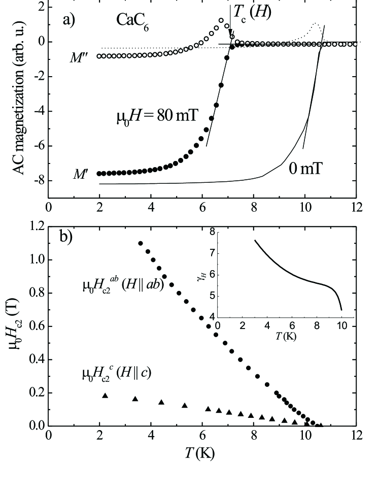
Figure 1: a) AC magnetization curves of CaC₆ taken at $\mu_{0}H=$ 80 mT and 0 mT. $M^{\prime}$ and $M^{\prime\prime}$ denote the real and the imaginary part of the AC magnetization, respectively. The arrow indicates the onset criterion to determine $T_{\text{c}}(H)$ (crossing of the two lines). b) Temperature dependence of the upper critical fields $H_{\text{c2}}^{c}$ and $H_{\text{c2}}^{ab}$ for the external magnetic field $H$$|$$|$$c$ and $H$$|$$|$$ab$, respectively, as determined by AC magnetization. The inset shows the calculated upper critical field anisotropy $\gamma_{H}=H_{\text{c2}}^{ab}/H_{\text{c2}}^{c}$ as a function of temperature.

To characterise our sample we carried out detailed AC magnetization measurements presented in Fig. 1. The AC component of the applied magnetic field was 1 mT at 1 kHz. Figure 1a shows typical AC magnetization curves at 80 mT (real $M^{\prime}(T)$ and imaginary $M^{\prime\prime}(T)$ part), the straight lines indicate the onset criterion to determine $T_{\text{c}}$. The temperature dependence of the upper critical field components $H_{\text{c2}}^{c}$ ($H$$|$$|$$c$) and $H_{\text{c2}}^{ab}$ ($H$$|$$|$$ab$) are displayed in Fig. 1b. The values of the $H_{\text{c2}}^{c}$ and $H_{\text{c2}}^{ab}$ were determined from AC magnetization using the procedure illustrated in Fig. 1a. The upper critical field is anisotropic and follows the temperature dependence as reported in Refs. critical_field and Cubitt_n . In the framework of the anisotropic Ginzburg-Landau theory the upper critical field for $H$$|$$|$$c$ and $H$$|$$|$$ab$ is given by

$$\mu_{0}H_{\text{c2}}^{ab}\left(0\right) = \frac{\Phi_{0}}{2\pi\xi_{ab}\left(0\right)\xi_{c}\left(0\right)},$$

$$\mu_{0}H_{\text{c2}}^{c}\left(0\right) = \frac{\Phi_{0}}{2\pi\xi_{ab}^{\text{2}}\left(0\right)},$$ (1)

where $\Phi_{0}=h/2e=2.07\cdot 10^{-15}$ Tm² is the flux quantum, and $\xi_{ab\text{,}c}$ are the corresponding coherence length components at zero temperature. With the linearly extrapolated values of the upper critical field at zero temperature, $\mu_{0}H_{\text{c2}}^{ab}\left(0\right)=2.1(3)$ T and $\mu_{0}H_{\text{c2}}^{c}\left(0\right)=0.25(2)$ T, and the equation above we obtain $\xi_{ab}\left(0\right)=36.3(1.5)$ nm and $\xi_{c}\left(0\right)=4.3(7)$ nm. These values are comparable to earlier reports such as resistivity measurements ($\xi_{ab}\left(0\right)=29.0$ nm and $\xi_{c}\left(0\right)=5.7$ nm) critical_field , or susceptibility studies ($\xi_{ab}\left(0\right)=35$ nm and $\xi_{c}\left(0\right)=13$ nm) Emery_susc . Remarkably, the upper critical field $H_{\text{c2}}^{ab}$ shows a positive curvature in the studied temperature region which was not observed in previous investigations. A similar positive curvature was observed near $T_{\text{c}}$ in MgB₂ mgb2poscurve where it was explained by a two-gap model. However, we should keep in mind that other explanations are also possible. Complementary experiments, such as studies of the superfluid density, as performed in this work, are necessary to draw definite conclusions.

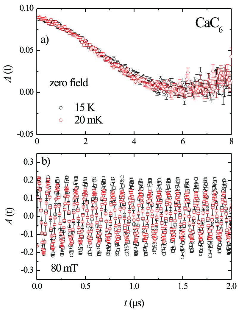
Figure 2: (color online) Measured $\mu$SR asymmetries $A(t)$ in CaC₆. a) Asymmetry in zero magnetic field (ZF). b) Asymmetry in 80 mT transverse field (TF). The black data points were taken at 15 K (well above $T_{\text{c}}$) and the red ones at 20 mK.

The temperature dependence of the upper critical field anisotropy $\gamma_{H}=$ $H_{\text{c2}}^{ab}/H_{\text{c2}}^{c}$ is shown in the inset of Fig. 1b. We interpolated the measured upper critical field values with a third order polynomial and determined the ratio $\gamma_{H}$. The anisotropy paremeter $\gamma_{H}$ increases monotonically with decreasing temperature, showing a similar temperature dependence as with MgB₂ mgb2torque . Note that a single gap isotropic $s$-wave description of superconductivity cannot account for this behaviour of $\gamma_{H}\left(T\right)$.

$\mu$SR experiments were carried out at the $\pi$M3 beamline using the GPS (General Purpose Spectrometer) and the LTF (Low Temperature Facility) spectrometers at the Paul Scherrer Institute PSI Villigen, Switzerland. Six pieces of CaC₆ forming an area of $\simeq$ 10x14 mm² were used in the experiment. In the intercalation process the Ca atoms penetrate from the side of the graphite sample and diffuse along the $ab$-plane. Reducing the sample size in the $ab$-direction favors Ca diffusion, and consequently leads to a higher sample quality than just using one large piece. For the LTF experiments the samples were glued on a silver plate with the help of Apiezon N grease and covered by silver coated polyester foil. In contrast, for the GPS experiments the samples were supported between the two arms of a specially designed fork by means of kapton tape. This technique allows only the incoming muons that stop in the sample to be counted, and therefore the background signal is reduced.

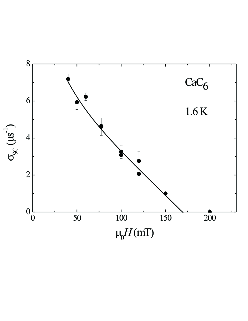
Figure 3: Field dependence of the Gaussian relaxation rate $\sigma_{\text{SC}}$ in CaC₆ measured at $T=1.6$ K. The solid line corresponds to the calculated curve using Eq. (3) (see text).

The magnetic field (80 mT) was applied along the crystallographic $c$-direction at 15 K well above $T_{\text{c}}.$ Then the sample was cooled down to the lowest temperature (20 mK for the LTF spectrometer), and $\mu$SR spectra were recorded with increasing temperature. The same procedure was applied in the GPS spectrometer, down to the lowest temperature of 1.6 K available in this device. The initial spin polarization of the implanted muons is perpendicular to the applied magnetic field $H$. The $\mu$SR experiments were performed at $H>H_{\text{c1}}^{\text{c}}$ so the sample was in the vortex state. Magnetic field dependent measurements were performed in the GPS spectrometer. At each magnetic field $H$ the sample was warmed up to 15 K (well above $T_{\text{c}}$), a $\mu$SR time spectrum was recorded, then it was cooled down to 1.6 K, and another $\mu$SR time spectrum was taken.Before and after the $\mu$SR experiments the same piece of CaC₆ was measured in the AC susceptometer, comparing the two measurements we observed no difference.

In the vortex state of a type II superconductor the muons probe the local magnetic field distribution $P(B)$ due to the vortex lattice field_dist . From the second moment $\langle\Delta B^{2}\rangle$ of $P(B)$ the in-plane magnetic penetration depth $\lambda_{ab}$ can be extracted according to the relation $\langle\Delta B^{2}\rangle=C\lambda_{ab}^{-2}$ ($C$ is a field dependent quantity) from which the superfluid density $\rho_{\text{s}}\propto\lambda_{ab}^{-2}$ can be determined Brandt_num . Thus, $\mu$SR provides a direct method to measure the superfluid density in the mixed state of a type II superconductor. Figure 2a shows the $\mu$SR asymmetries $A(t)$ recorded in LTF in zero magnetic field above $T_{\text{c}}$ and at 20 mK. The two time spectra overlap, indicating the absence of any kind of magnetic order in the sample and in the sample holder. The time dependence of the asymmetry can be described by the static Kubo-Toyabe formula, showing only the presence of randomly distributed nuclear magnetic moments, but no realization of magnetism. Figure 2b shows the $\mu$SR asymmetries taken at 15 K well above $T_{\text{c}}\simeq 11.5$ K and at 20 mK in a field of 80 mT. A clear damping of the $\mu$SR signal at 20 mK due to the presence of the vortex lattice is visible. For a detailed description of $\mu$SR studies of the vortex state in type II superconductors see, e.g. field_dist . The $\mu$SR time spectra were fitted to the following expression:

$$A^{\text{TF}}(t) = A_{\text{SC}}e^{(\sigma_{\text{SC}}t)^{2}/2}\cos(\gamma_{\mu}B_{\text{SC}}+\phi)$$ (2)

$$+A_{\text{bg}}e^{(\sigma_{\text{bg}}t)^{2}/2}\cos(\gamma_{\mu}B_{\text{bg}}+\phi)$$

$$+A_{\text{Ag}}\cos(\gamma_{\mu}B_{\text{Ag}}+\phi)$$

Here the indices SC, bg and Ag denote the sample (superconductor), the background arising from non superconducting parts of the sample and the non-relaxing silver background, respectively. $A$ denotes the initial asymmetry, $\sigma$ is the Gaussian relaxation rate, $\gamma_{\mu}=2\pi\cdot 135.5342$ MHz/T is the muon gyromagnetic ratio, $B$ is the internal magnetic field, and $\phi$ is the initial phase of the moun-spin ensemble. A set of $\mu$SR data were fitted simultaneously with $A_{\text{SC}}$, $A_{\text{bg}}$, $A_{\text{Ag}}$, $B_{\text{bg}}$, $B_{\text{Ag}}$, $\sigma_{\text{bg}}$, and $\phi$ as common parameters, and $B_{\text{SC}}$ and $\sigma_{\text{SC}}$ as free parameters for each temperature. The same expression was used to analyse the data recorded with the GPS spectrometer (where no silver background signal is present). To analyze the magnetic field dependent $\mu$SR measurements $B_{\text{SC}}$ was a free parameter in Eq. (2) since it depends on the applied field.

The analysis of the field dependence of the measured $\mu$SR relaxation rate $\sigma_{\text{SC}}\propto$ $\langle\Delta B^{2}\rangle$ allows to estimate the absolute value of the in-plane magnetic penetration depth $\lambda_{\text{ab}}$, assuming that CaC₆ can be described as a single isotropic $s$-wave gap superconductor. The measured values of $\sigma_{\text{SC}}$ are plotted in Fig. 3. To analyze our data we used the formula developed by Brandt Brandt_num :

$$\sigma_{\text{SC}}\simeq 0.172\gamma_{\mu}\frac{\Phi_{0}}{2\pi}\left(1-\frac{B}{B_{\text{c2}}^{c}}\right)\left[1+1.21\left(1-\sqrt{\frac{B}{B_{\text{c2}}^{c}}}\right)^{3}\right]\lambda_{ab}^{-2}\text{.}$$ (3)

Although the formula was derived for high $\kappa$ type II superconductors ($\kappa\geq 5$), it was suggested to work also for low values of $\kappa$ at magnetic fields $\sqrt{B/B_{\text{c2}}^{c}}\geq 0.5$ DiCastro . From the measured $\mu$SR relaxation rates $\sigma_{\text{SC}}$ and Eq. (3) one obtains $\lambda_{ab}\left(0\right)=78(3)$ nm and $B_{\text{c2}}^{c}(0)=170(5)$ mT. The solid line in Fig. 3 represents the corresponding fit (the point at 200 mT was not included in the fit). To estimate the Ginzburg-Landau parameter $\kappa$ we use our values of $\xi_{ab}\left(0\right)=36.3(1.5)$ nm and $\lambda_{ab}\left(0\right)=78(3)$ nm giving $\kappa\approx 2.1$. It is worth to mention that the value of $B_{\text{c2}}^{\text{c}}$ is smaller than that estimated from the AC magnetization measurements ($B_{\text{c2}}^{c}(0)\simeq 250$ mT), since AC magnetization measurements resulted more data points to determine the upper critical field value we take 250 mT as $B_{\text{c2}}^{c}(0)$ for the further analysis.

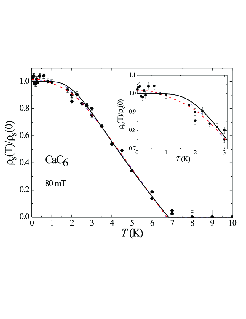
Figure 4: (color online) Temperature dependence of the normalized superfluid density $\rho_{\text{s}}(T)/\rho_{\text{s}}(0)$ in CaC₆ measured at 80 mT. The inset shows the low temperature region. The black line corresponds to a single-gap isotropic $s$-wave, the blue, dotted line to a single-gap anisotropic $s$-wave, and the red, dashed line to a two-gap isotropic $s$-wave description of $\rho_{\text{s}}(T)$. For a detailed explanation see text.

It is generally assumed that the superfluid density $\rho_{\text{S}}$ is related to the in-plane magnetic penetration depth $\lambda_{\text{ab}}$ by the simple relation $\rho_{\text{S}}\propto\lambda_{\text{ab}}^{-2}$. However, for magnetic fields close to $B_{\text{c2}}$ this proportionality must be corrected because the order parameter $\psi\left(r\right)$ is reduced due to the overlapping vortices. In this case the spatial average of the superfluid density is given by DiCastro :

$$\rho_{\text{s}}\left(T\right)\simeq\langle|\psi\left(r\right)|^{2}\rangle\lambda^{-2}\left(T\right)\simeq\left(1-B/B_{\text{c2}}^{c}(T)\right)\lambda_{ab}^{-2}\left(T\right),$$ (4)

where $\langle...\rangle$ means the spatial average. Values of $\lambda_{ab}^{-2}$  were calculated using Eq. (3) and for the values of $B_{\text{c2}}^{c}$ we used the results of our AC magnetization measurements (see Fig. 1b). The temperature dependence of the superfluid density $\rho_{\text{s}}\left(T\right)$ determined at 80 mT is plotted in Fig. 4. We analyzed $\rho_{\text{s}}\left(T\right)$ using three different models: i) single-gap isotropic $s$-wave ii) single-gap anisotropic $s$-wave, and iii) two-gap isotropic $s$-wave. To calculate the temperature dependence of the magnetic penetration depth within the local approximation ($\lambda\gg\xi$) we applied the following formula gap1 ; gap2 :

$$\rho_{\text{s}}\left(T\right)=\rho_{\text{s}}\left(0\right)\left(1+\frac{1}{\pi}\int_{0}^{2\pi}\int_{\Delta\left(T,\phi\right)}^{\infty}\left(\frac{\partial f}{\partial E}\right)\frac{E\text{ }dEd\phi}{\sqrt{E^{2}-\Delta\left(T,\phi\right)^{2}}}\right)\text{,}$$ (5)

where $\rho_{\text{S}}\left(0\right)$ is the zero temperature value of the superfluid density, $f=\left[1+\exp\left((E-E_{\text{F}})/k_{\text{B}}T\right)\right]^{-1}$ is the Fermi function, $\phi$ is the angle along the Fermi surface, and $\Delta\left(T,\phi\right)=\Delta_{0}h\left(T/T_{\text{c}}\right)g\left(\phi\right)$. The temperature dependence of the gap is expressed by $h\left(T/T_{\text{c}}\right)=\tanh\left(1.82\left[1.018\left(T_{\text{c}}/T-1\right)\right]^{0.51}\right)$ gap3 . For the isotropic $s$-wave gap i) $g^{\text{s}}\left(\phi\right)=1$ and for the anisotropic $s$-wave gap ii) $g^{\text{s}_{\text{An}}}\left(\phi\right)=\left(1+a\cos 4\phi\right)/\left(1+a\right)$, where $a$ denotes the anisotropy of the gap. The two-gap fit was calculated using the so called $\alpha$-model and assuming that the total superfluid density is the sum of the two components gap2 ; gap3 :

$$\rho_{\text{s}}\left(T\right)=\rho_{\text{s}}\left(0\right)\left(\omega\frac{\rho\left(T,\Delta_{0,1}\right)}{\rho\left(0,\Delta_{0,1}\right)}+\left(1-\omega\right)\frac{\rho\left(T,\Delta_{0,2}\right)}{\rho\left(0,\Delta_{0,2}\right)}\right)\text{.}$$ (6)

Here $\Delta_{0,1}$ and $\Delta_{0,2}$ are the zero temperature values of the larger and the smaller gap, and $\omega$ $\left(0\leq\omega\leq 1\right)$ is a weighting factor representing the relative contribution of the larger gap to $\rho_{\text{s}}$. The results obtained for the different models are plotted in Fig. 4. The black line represents the result for the single $s$-wave gap model i) with $\rho_{\text{s}}\left(0\right)=96.5(5)$ $\mu$m^-2, $\Delta_{0}=0.79(1)$ meV, $T_{\text{c}}=6.80(2)$ K, and $2\Delta_{0}/k_{\text{B}}T_{\text{c}}=2.70(5)$, describing CaC₆ as weak coupling BCS superconductor. The reduction of $T_{\text{c}}$ agrees well with our AC magnetization measurements for 80 mT. The blue, dotted line represents the anisotropic $s$-wave gap analysis ii) with $\Delta_{0}=0.81(1)$ meV and $a\simeq 0.37$ for the gap anisotropy. These values do not agree with the reported ones from tunneling experiments ($\Delta_{0}^{c}\simeq 1.7$ meV and $\Delta_{0}^{ab}\simeq 1.44$ meV) pointcontact . The two-gap analysis iii) (red, dashed line) yields $\Delta_{0,1}=0.85(2)$ meV for the larger gap and $\Delta_{0,2}=0.23(1)$ meV for the smaller one. Only $\sim 9.4(3)$ % of the superfluid density is associated with the smaller gap. The smaller gap agrees with $\Delta_{0,2}=0.2(2)$ meV reported in arpes . Our larger gap value is significantly smaller ($\Delta_{0,1}=1.9(2)$ meV). It is worth to mention that the applicability of the two gap model at this magnetic field (80 mT) is questionable. The gap magnitude scales with the upper critical field, $\left(\frac{\Delta_{0,1}}{\Delta_{0,2}}\right)^{2}\sim\frac{B_{\text{c2}}^{1}}{B_{\text{c2}}^{2}},$ resulting $B_{\text{c2}}^{2}\sim 12$ mT which is much smaller than the applied magnetic field. Although the best agreement is found for the two-gap scenario, no final conclusion can be drawn from this analysis. All three scenarios describe well the observed temperature dependence of the superfluid density. For a direct comparison with Ref. DiCastro we omitted the values of $\rho_{\text{s}}\left(T\right)$ below 2 K. In this case the single s-wave gap fit yields $\rho_{\text{s}}\left(0\right)=91.6(9)$ $\mu$m^-2, $\Delta_{0}=0.84(1)$ meV, $T_{\text{c}}=6.75(2)$ K, and $2\Delta_{0}/k_{\text{B}}T_{\text{c}}=2.90(5)$. The values presented in Ref. DiCastro are: $\rho_{\text{s}}\left(0\right)=85.1(3)$ $\mu$m^-2, $\Delta_{0}=0.868(5)$ meV, and $2\Delta_{0}/k_{\text{B}}T_{\text{c}}=3.6(1)$. The higher applied magnetic field (120 mT in Ref. DiCastro ) may account for the differences. Here, one should point out that our low temperature data are essential to determine the zero temperature values of $\rho_{\text{s}}$ and $\Delta$.

III Conclusions

In conlusion, we carried out extensive AC magnetization measurements to map the temperature dependence of the upper critical field $H_{\text{c2}}^{ab}$ and $H_{\text{c2}}^{c}$ in CaC₆ and to evaluate the coherence length. The values of $\xi_{ab}\left(0\right)=36.3(1.5)$ nm and $\xi_{c}\left(0\right)=4.3(7)$ nm are in good agreement with those reported previously critical_field ; Emery_susc . We found that the upper critical field anisotropy $\gamma_{H}=$ $H_{\text{c2}}^{ab}/H_{\text{c2}}^{c}$ increases with decreasing temperature. From magnetic field dependent $\mu$SR experiments the absolute value of the in-plane magnetic penetration depth was determined to be $\lambda_{ab}\simeq 78(3)$ nm, in agreement with previously reported values LamuraPRL ; DiCastro . Furthermore, low temperature $\mu$SR experiments were performed in order to map the whole temperature dependence of the superfluid density $\rho_{\text{s}}\left(T\right)$. We analyzed the temperature dependence of $\rho_{\text{s}}$ with three different models: i) single-gap isotropic $s$-wave, ii) single-gap anisotropic $s$-wave, and iii) two-gap isotropic $s$-wave. All models describe the measured $\mu$SR data almost equally well, although a slightly better agreement was achieved using the two-gap model.

This work was partly supported by the Swiss National Science Foundation (SCOPES grant No. IZ73Z0_128242). The $\mu$SR experiments were performed at the Swiss Muon Source, Paul Scherrer Institut, Villigen, Switzerland.

References

- (1) T. E. Weller, M. Ellerby, S. S. Saxena, R. P. Smith, and N. T. Skipper, Nature Physics 1, 39 (2005).
- (2) N. B. Hannay, T. H. Geballe, B. T. Matthias, K. Andres, P. Schmidt, and D. MacNair, Phys. Rev. Lett. 14, 225 (1965).
- (3) R. A. Wachnik, L. A. Pendrys, F. L. Vogel, and P. Lagrange, Solid State Comm. 43, 5 (1982).
- (4) I. T. Belash, A. D. Bronnikov, O. V. Zharikov, and A. V. Pal’nichenko, Synth. Met. 36, 283 (1990).
- (5) V. V. Avdeev, O. V. Zharikov, V. A. Nalimova, A. V. Pal’nichenko, and K. N. Semenenko, Zh. Eksp. Teor. Fiz. 43, 376 (1986).
- (6) N. Bergeal, V. Dubost, Y. Noat, W. Sacks, D. Roditchev, N. Emery, C. H rold, J-F. Mar ch , P. Lagrange, and G. Loupias, Phys. Rev. Lett. 97, 077003 (2006).
- (7) G. Lamura, M. Aurino, G. Cifariello, E. Di Gennaro, A. Andreone, N. Emery, C. H rold, J.-F. Mar ch , and P. Lagrange, Phys. Rev. Lett. 96, 107008 (2006).
- (8) E. Jobiliong, H. D. Zhou, J. A. Janik, Y.-J. Jo, L. Balicas, J. S. Brooks, and C. R. Wiebe, Phys. Rev. B 76, 052511 (2007).
- (9) K. Sugawara, T. Sato, and T. Takahashi, Nat. Phys. 5, 40 (2009).
- (10) R. S. Gonnelli, D. Daghero, D. Delaude, M. Tortello, G. A. Ummarino, V. A. Stepanov, J. S. Kim, R. K. Kremer, A. Sanna, G. Profeta, and S. Massidda, Phys. Rev. Lett. 100, 207004 (2008).
- (11) R. Khasanov, S. Str ssle, D. Di Castro, T. Masui, S. Miyasaka, S. Tajima, A. Bussmann-Holder, and H. Keller, Phys. Rev. Lett. 99, 237601 (2007).
- (12) D. Di Castro, A. Kanigel, A. Maisuradze, A. Keren, P. Postorino, D. Rosenmann, U. Welp, G. Karapetrov, H. Claus, D. G. Hinks, A. Amato, and J. C. Campuzano, Phys. Rev. B 82, 014530 (2010).
- (13) N. Emery, C. H rold, and P. Lagrange, J. Solid State Chem. 178, 2947 (2005).
- (14) R. Cubitt, J. S. White, M. Laver, M. R. Eskildsen, C. D. Dewhurst, D. McK. Paul, A. J. Crichton, M. Ellerby, C. Howard, Z. Kurban, and F. Norris, Phys. Rev. B 75, 140516(R) (2007).
- (15) N. Emery, C. H rold, M. d’Astuto, V. Garcia, Ch. Bellin, J. F. Mar ch , P. Lagrange, and G. Loupias, Phys. Rev. Lett. 95, 087003 (2005).
- (16) H. Suderow, V. G. Tissen, J. P. Brison, J. L. Mart nez, S. Vieira, P. Lejay, S. Lee, and S. Tajima, Phys. Rev. B 70, 134518 (2004).
- (17) M. Angst, R. Puzniak, A. Wisniewski, J. Jun, S. M. Kazakov, J. Karpinski, J. Roos, and H. Keller, Phys. Rev. Lett. 88, 167004 (2002).
- (18) A. Maisuradze, R. Khasanov, A. Shengelaya and H. Keller, J. Phys.: Condens. Matter 21, 075701 (2009).
- (19) E. H. Brandt, Phys. Rev. B 68, 054506 (2003).
- (20) M. Tinkham, Introduction to Superconductivity, Krieger Publishing Company, Malabar, Florida (1975).
- (21) R. Khasanov, A. Shengelaya, A. Maisuradze, F. La Mattina, A. Bussmann-Holder, H. Keller, and K. A. M ller, Phys. Rev. Lett. 98, 057007 (2007).
- (22) A. Carrington and F. Manzano, Physica C 385, 205 (2003).