Statistical Multiresolution Dantzig Estimation in Imaging: Fundamental Concepts and Algorithmic Framework

Klaus Frick Institute for Mathematical Stochastics
University of Göttingen
Goldschmidtstraße 7, 37077 Göttingen
frick@math.uni-goettingen.de
Philipp Marnitz Institute for Mathematical Stochastics
University of Göttingen
Goldschmidtstraße 7, 37077 Göttingen
marnitz@math.uni-goettingen.de
 and  Axel Munk Institute for Mathematical Stochastics
University of Göttingen
Goldschmidtstraße 7, 37077 Göttingen
and
Max Planck Institute for Biophysical Chemistry
Am Faßberg 11, 37077 Göttingen
munk@math.uni-goettingen.de
Abstract.

In this paper we are concerned with fully automatic and locally adaptive estimation of functions in a “signal ++ noise”-model where the regression function may additionally be blurred by a linear operator, e.g. by a convolution. To this end, we introduce a general class of statistical multiresolution estimators and develop an algorithmic framework for computing those. By this we mean estimators that are defined as solutions of convex optimization problems with subscript\ell_{\infty}-type constraints. We employ a combination of the alternating direction method of multipliers with Dykstra’s algorithm for computing orthogonal projections onto intersections of convex sets and prove numerical convergence. The capability of the proposed method is illustrated by various examples from imaging and signal detection.

Key words and phrases:
Alternating Direction Method of Multipliers (ADMM), Biophotonics, Dantzig Selector, Dykstra’s Projection Algorithm, Statistical Imaging, Statistical Multiscale Analysis, Statistical Regularization, Local Adaption, Signal Detection
2000 Mathematics Subject Classification:
Primary: 62G05, 90C06; secondary 68U10
Correspondence to frick@math.uni-goettingen.de

1. Introduction

In numerous applications, the relation of observable data Y𝑌Y and the (unknown) signal of interest u0superscript𝑢0u^{0} can be modeled as an inverse linear regression problem. We shall assume that the data Y={Y𝝂}𝑌subscript𝑌𝝂Y=\left\{Y_{\mathchoice{\mbox{\boldmath$\displaystyle\nu$}}{\mbox{\boldmath$\textstyle\nu$}}{\mbox{\boldmath$\scriptstyle\nu$}}{\mbox{\boldmath$\scriptscriptstyle\nu$}}}\right\} is sampled on the equidistant grid X={1,,m}d𝑋superscript1𝑚𝑑X=\left\{1,\dots,m\right\}^{d}, with m,d𝑚𝑑m,d\in\mathbb{N} and that u0Usuperscript𝑢0𝑈u^{0}\in U for some linear space U𝑈U, such as the Euclidean space or a Sobolev class of functions. Hence the model can be formalized as

Y𝝂=(Ku0)𝝂+ε𝝂,𝝂X.formulae-sequencesubscript𝑌𝝂subscript𝐾superscript𝑢0𝝂subscript𝜀𝝂𝝂𝑋Y_{\mathchoice{\mbox{\boldmath$\displaystyle\nu$}}{\mbox{\boldmath$\textstyle\nu$}}{\mbox{\boldmath$\scriptstyle\nu$}}{\mbox{\boldmath$\scriptscriptstyle\nu$}}}=(Ku^{0})_{\mathchoice{\mbox{\boldmath$\displaystyle\nu$}}{\mbox{\boldmath$\textstyle\nu$}}{\mbox{\boldmath$\scriptstyle\nu$}}{\mbox{\boldmath$\scriptscriptstyle\nu$}}}+\varepsilon_{\mathchoice{\mbox{\boldmath$\displaystyle\nu$}}{\mbox{\boldmath$\textstyle\nu$}}{\mbox{\boldmath$\scriptstyle\nu$}}{\mbox{\boldmath$\scriptscriptstyle\nu$}}},\quad\mathchoice{\mbox{\boldmath$\displaystyle\nu$}}{\mbox{\boldmath$\textstyle\nu$}}{\mbox{\boldmath$\scriptstyle\nu$}}{\mbox{\boldmath$\scriptscriptstyle\nu$}}\in X. (1)

Here we assume that ε={ε𝝂}𝝂X𝜀subscriptsubscript𝜀𝝂𝝂𝑋\varepsilon=\left\{\varepsilon_{\mathchoice{\mbox{\boldmath$\displaystyle\nu$}}{\mbox{\boldmath$\textstyle\nu$}}{\mbox{\boldmath$\scriptstyle\nu$}}{\mbox{\boldmath$\scriptscriptstyle\nu$}}}\right\}_{\mathchoice{\mbox{\boldmath$\displaystyle\nu$}}{\mbox{\boldmath$\textstyle\nu$}}{\mbox{\boldmath$\scriptstyle\nu$}}{\mbox{\boldmath$\scriptscriptstyle\nu$}}\in X} are independent and identically distributed r.v. with 𝐄(ε𝝂)=0𝐄subscript𝜀𝝂0\mathbf{E}\left(\varepsilon_{\mathchoice{\mbox{\boldmath$\displaystyle\nu$}}{\mbox{\boldmath$\textstyle\nu$}}{\mbox{\boldmath$\scriptstyle\nu$}}{\mbox{\boldmath$\scriptscriptstyle\nu$}}}\right)=0 and 𝐄(ε𝝂2)=σ2>0𝐄superscriptsubscript𝜀𝝂2superscript𝜎20\mathbf{E}\left(\varepsilon_{\mathchoice{\mbox{\boldmath$\displaystyle\nu$}}{\mbox{\boldmath$\textstyle\nu$}}{\mbox{\boldmath$\scriptstyle\nu$}}{\mbox{\boldmath$\scriptscriptstyle\nu$}}}^{2}\right)=\sigma^{2}>0 (white noise). Moreover, K:U(m)d:𝐾𝑈superscriptsuperscript𝑚𝑑K:U\rightarrow(\mathbb{R}^{m})^{d} denotes a linear operator that encodes the functional relation between the quantities that are accessible by experiment and the underlying signal. Often the operator K𝐾K does not have a continuous inverse (or its inverse is ill-conditioned in a discrete setting, where K𝐾K is a matrix), that is estimation of u0superscript𝑢0u^{0} given the data Y𝑌Y is an ill-posed problem. As a consequence, estimators for u0superscript𝑢0u^{0} can not be obtained by merely applying the inverse of K𝐾K to an estimator of Ku0𝐾superscript𝑢0Ku^{0}, in general. Instead, more sophisticated statistical regularization techniques have to be employed that, loosely speaking, are capable of simultaneously inverting K𝐾K and solving the regression problem.

The application we primarily have in mind is the reconstruction of low-dimensional signals (e.g. images) u0superscript𝑢0u^{0} which are presumed to exhibit a strong neighborhood structure as it is characteristic for imaging or signal detection problems. These neighborhood relations are often modeled by prior smoothness or structural assumptions on u0superscript𝑢0u^{0} (e.g. on the texture of an image).

The aim of this paper is twofold. First, we will introduce the broad class of statistical multiresolution estimators (SMRE). We claim that numerous regularization techniques, that were recently proposed for different problems in various branches of applied mathematics and statistics, can be considered as special cases of these. Among others, this includes the Dantzig selector (see [4, 7, 29] and references therein) that was recently proposed in the context of high dimensional statistics. Our prior focus, however, will be put on imaging problems and it will turn out that the aforementioned neighborhood relations can be modeled within our SMRE framework in a straightforward manner. This will result in locally adaptive and fully automatic image reconstruction methods.

The high intrinsic structure of the signals that are typically under consideration in imaging is in contrast to the usual situation in high-dimensional statistics. Here u0superscript𝑢0u^{0} is usually assumed to be unstructured but to have a sparse representation with respect to some basis of U𝑈U (cf. [43, 8, 7]). Consequently, the consistent estimation of u0superscript𝑢0u^{0} is realized by minimizing a regularization functional which fosters sparsity, such as the 1subscript1\ell_{1}-norm of the coefficients, subject to an subscript\ell_{\infty}-constraint on the coefficients of the residual, i.e.

infuUu1 s.t. K(YKu)q.subscriptinfimum𝑢𝑈subscriptnorm𝑢1 s.t. subscriptnormsuperscript𝐾𝑌𝐾𝑢𝑞\inf_{u\in U}\left\|u\right\|_{1}\quad\text{ s.t. }\quad\left\|K^{*}(Y-Ku)\right\|_{\infty}\leq q. (2)

In order to apply this approach for image reconstruction, two modifications become necessary: Often one aims to minimize other regularization functionals such as the total variation semi-norm (cf. [34, 37]) or Sobolev norms, say. Hence, we suggest to replace the 1subscript1\ell_{1}-norm in (2) by a general convex functional J𝐽J that models the smoothness or texture information of signals or images (cf. [1, 35]). Furthermore, we relax the subscript\ell_{\infty}-constraint such that neighborhood relations of the image can be taken into account. This generalizes the Dantzig selector to this task in a natural way and obviously increases estimation efficientcy. As we will layout in Paragraph 1.2.2, this requires new algorithms to compute efficiently the resulting large scale optimization problem.

1.1. Statistical Multiresolution Estimation

We will now introduce the announced class of estimators. To this end, let 𝒮𝒮\mathcal{S} be some index set and 𝒲={ωS:S𝒮}𝒲conditional-setsuperscript𝜔𝑆𝑆𝒮\mathcal{W}=\left\{\omega^{S}~{}:~{}S\in\mathcal{S}\right\} be a set of given weight-functions on the grid X={1,,m}d𝑋superscript1𝑚𝑑X=\left\{1,\ldots,m\right\}^{d}. A statistical multiresolution estimator (SMRE) (or generalized Dantzig selector), is defined as a solution of the constrained optimization problem

infuUJ(u) s.t. maxS𝒮|𝝂Xω𝝂S(Λ(YKu))𝝂|q.subscriptinfimum𝑢𝑈𝐽𝑢 s.t. subscript𝑆𝒮subscript𝝂𝑋subscriptsuperscript𝜔𝑆𝝂subscriptΛ𝑌𝐾𝑢𝝂𝑞\inf_{u\in U}J(u)\quad\text{ s.t. }\quad\max_{S\in\mathcal{S}}\left|\sum_{\mathchoice{\mbox{\boldmath$\displaystyle\nu$}}{\mbox{\boldmath$\textstyle\nu$}}{\mbox{\boldmath$\scriptstyle\nu$}}{\mbox{\boldmath$\scriptscriptstyle\nu$}}\in X}\omega^{S}_{\mathchoice{\mbox{\boldmath$\displaystyle\nu$}}{\mbox{\boldmath$\textstyle\nu$}}{\mbox{\boldmath$\scriptstyle\nu$}}{\mbox{\boldmath$\scriptscriptstyle\nu$}}}\left(\Lambda(Y-Ku)\right)_{\mathchoice{\mbox{\boldmath$\displaystyle\nu$}}{\mbox{\boldmath$\textstyle\nu$}}{\mbox{\boldmath$\scriptstyle\nu$}}{\mbox{\boldmath$\scriptscriptstyle\nu$}}}\right|\leq q. (3)

Here, J:U:𝐽𝑈J:U\rightarrow\mathbb{R} denotes a regularization functional that incorporates a priori knowledge on the unknown signal u0superscript𝑢0u^{0} (such as smoothness) and Λ:(m)d(m)d:Λsuperscriptsuperscript𝑚𝑑superscriptsuperscript𝑚𝑑\Lambda:(\mathbb{R}^{m})^{d}\rightarrow(\mathbb{R}^{m})^{d} a possibly non-linear transformation. The constant q𝑞q can be considered as a universal regularization parameter that governs the trade-off between regularity and data-fit of the reconstruction. In most practical situations q𝑞q is chosen to be the α𝛼\alpha-quantile qαsubscript𝑞𝛼q_{\alpha} of the multiresolution (MR) statistic T(ε)𝑇𝜀T(\varepsilon), where T:(m)d:𝑇superscriptsuperscript𝑚𝑑T:(\mathbb{R}^{m})^{d}\rightarrow\mathbb{R} encodes the inequality constraint in (3), i.e.

T(v)=maxS𝒮|𝝂Xω𝝂S(Λ(v))𝝂|,v(m)d.formulae-sequence𝑇𝑣subscript𝑆𝒮subscript𝝂𝑋subscriptsuperscript𝜔𝑆𝝂subscriptΛ𝑣𝝂𝑣superscriptsuperscript𝑚𝑑T(v)=\max_{S\in\mathcal{S}}\left|\sum_{\mathchoice{\mbox{\boldmath$\displaystyle\nu$}}{\mbox{\boldmath$\textstyle\nu$}}{\mbox{\boldmath$\scriptstyle\nu$}}{\mbox{\boldmath$\scriptscriptstyle\nu$}}\in X}\omega^{S}_{\mathchoice{\mbox{\boldmath$\displaystyle\nu$}}{\mbox{\boldmath$\textstyle\nu$}}{\mbox{\boldmath$\scriptstyle\nu$}}{\mbox{\boldmath$\scriptscriptstyle\nu$}}}\left(\Lambda(v)\right)_{\mathchoice{\mbox{\boldmath$\displaystyle\nu$}}{\mbox{\boldmath$\textstyle\nu$}}{\mbox{\boldmath$\scriptstyle\nu$}}{\mbox{\boldmath$\scriptscriptstyle\nu$}}}\right|,\quad v\in(\mathbb{R}^{m})^{d}. (4)

To this end, we assume the distribution of T(ε)𝑇𝜀T(\varepsilon) to be (approximately) known. This can either be obtained by simulations or in some cases the limiting distribution can even be derived explicitly. The regularization parameter q𝑞q then admits a sound statistical interpretation: Each solution u^αsubscript^𝑢𝛼\hat{u}_{\alpha} of (3) satisfies

(J(u^α)J(u0))α𝐽subscript^𝑢𝛼𝐽superscript𝑢0𝛼\mathbb{P}\left(J(\hat{u}_{\alpha})\leq J(u^{0})\right)\geq\alpha

i.e. the estimator u^αsubscript^𝑢𝛼\hat{u}_{\alpha} is more regular (in terms of J𝐽J) than u0superscript𝑢0u^{0} with a probability of at least α𝛼\alpha. To see this simply observe that the true signal u0superscript𝑢0u^{0} satisfies the constraint in (3) with probability at least α𝛼\alpha.

For a given estimator u^^𝑢\hat{u} of u0superscript𝑢0u^{0}, the set 𝒲𝒲\mathcal{W} is assumed to be rich enough in order to catch all relevant non-random signals that are visible in the residual YKu^𝑌𝐾^𝑢Y-K\hat{u}. Then, the average function

μS(v)=|𝝂Xω𝝂S(Λ(v))𝝂|subscript𝜇𝑆𝑣subscript𝝂𝑋subscriptsuperscript𝜔𝑆𝝂subscriptΛ𝑣𝝂\mu_{S}(v)=\left|\sum_{\mathchoice{\mbox{\boldmath$\displaystyle\nu$}}{\mbox{\boldmath$\textstyle\nu$}}{\mbox{\boldmath$\scriptstyle\nu$}}{\mbox{\boldmath$\scriptscriptstyle\nu$}}\in X}\omega^{S}_{\mathchoice{\mbox{\boldmath$\displaystyle\nu$}}{\mbox{\boldmath$\textstyle\nu$}}{\mbox{\boldmath$\scriptstyle\nu$}}{\mbox{\boldmath$\scriptscriptstyle\nu$}}}\left(\Lambda(v)\right)_{\mathchoice{\mbox{\boldmath$\displaystyle\nu$}}{\mbox{\boldmath$\textstyle\nu$}}{\mbox{\boldmath$\scriptstyle\nu$}}{\mbox{\boldmath$\scriptscriptstyle\nu$}}}\right| (5)

evaluated at v=YKu^𝑣𝑌𝐾^𝑢v=Y-K\hat{u} is supposed to be significantly larger than q𝑞q for at least one ω𝒲𝜔𝒲\omega\in\mathcal{W}, whenever YKu^𝑌𝐾^𝑢Y-K\hat{u} fails to resemble white noise. Put differently, the MR-statistic T(YKu^)𝑇𝑌𝐾^𝑢T(Y-K\hat{u}) is bounded by q𝑞q, whenever YKu^𝑌𝐾^𝑢Y-K\hat{u} is accepted as white noise according to the resolution provided by 𝒲𝒲\mathcal{W}. In fact, this is a key observations that reveals numerous potential application areas of the estimation method (3). The examples we have in mind are mainly from statistical signal detection and imaging, where the index set 𝒮𝒮\mathcal{S} is typically chosen to be an overlapping (redundant) system of subsets of the grid X𝑋X and ωSsuperscript𝜔𝑆\omega^{S} is the normalized indicator function on S𝒮𝑆𝒮S\in\mathcal{S}. Consequently the inequality constraint in (3) guarantees that the residual resembles white noise on all sets S𝒮𝑆𝒮S\in\mathcal{S}. In other words, the SMRE approach in (3) yields a reconstruction method that locally adapts the amount of regularization according to the underlying image features. We illustrate this in Section 3 by various examples.

Summarizing, the optimization problem in (3) amounts to choose the most parsimonious among all estimators u^^𝑢\hat{u} for which the residual YKu^𝑌𝐾^𝑢Y-K\hat{u} resembles white noise according to the statistic T𝑇T. If YKu^𝑌𝐾^𝑢Y-K\hat{u} contains some non randon signal, i.e. T(YKu^)𝑇𝑌𝐾^𝑢T(Y-K\hat{u}) is likely to be larger than q𝑞q and u𝑢u happens to lie outside the admissible domain of (3). Thus, the multi-resolution constraint prevents too parsimonious reconstructions due to the minimization of J𝐽J.

1.2. Algorithmic Challenges and Related Work

1.2.1. Multiresolution Methods

SMREs and related MR statistics have recently been studied in various contexts. We give a brief (but incomplete) overview.

Classical MR statistics are obtained from the general form in (4) by setting U=(m)d𝑈superscriptsuperscript𝑚𝑑U=(\mathbb{R}^{m})^{d} and Λ=IdΛId\Lambda=\textnormal{Id}. Moreover, one considers the system 𝒲𝒲\mathcal{W} to contain indicator functions on cubes. To be more precise, define the index set 𝒮𝒮\mathcal{S} to be the system of all d𝑑d-dimensional cubes in X𝑋X and set ωS=χS/#S.superscript𝜔𝑆subscript𝜒𝑆#𝑆\omega^{S}=\chi_{S}/\sqrt{\#S}. Then, the MR-statistic in (4) reduces to

T(v)=maxS𝒮1#S|𝝂Sv𝝂|.𝑇𝑣subscript𝑆𝒮1#𝑆subscript𝝂𝑆subscript𝑣𝝂T(v)=\max_{S\in\mathcal{S}}\frac{1}{\sqrt{\#S}}\left|\sum_{\mathchoice{\mbox{\boldmath$\displaystyle\nu$}}{\mbox{\boldmath$\textstyle\nu$}}{\mbox{\boldmath$\scriptstyle\nu$}}{\mbox{\boldmath$\scriptscriptstyle\nu$}}\in S}v_{\mathchoice{\mbox{\boldmath$\displaystyle\nu$}}{\mbox{\boldmath$\textstyle\nu$}}{\mbox{\boldmath$\scriptstyle\nu$}}{\mbox{\boldmath$\scriptscriptstyle\nu$}}}\right|.

This statistic was introduced in [42] (called scanning statistic there) in order to detect a signal against a noisy background. It was shown in [31] that

limmT(ε)2dlogm=σ a.s.subscript𝑚𝑇𝜀2𝑑𝑚𝜎 a.s.\lim_{m\rightarrow\infty}\frac{T(\varepsilon)}{\sqrt{2d\log m}}=\sigma\quad\text{ a.s.}

If the system 𝒮𝒮\mathcal{S} is reduced to the set of all dyadic squares, then it was proved in [28] that (after suitable transformations) T𝑇T also converges weakly to the Gumbel distribution. There, the authors also established a method for locally adaptive image denoising employing linear diffusion equations with spatially varying diffusivity. SMREs (3) have been studied recently for the case d=1𝑑1d=1 in [12] and [6], where total-variation penalty and the number of jumps in piecewise constant regression were considered as regularization functional J𝐽J, respectively. In [21] consistency and convergence rates for SMREs have been studied in a general Hilbert space setting.

SMREs with squared residuals, that is Λ(v)𝝂=v𝝂2Λsubscript𝑣𝝂superscriptsubscript𝑣𝝂2\Lambda(v)_{\mathchoice{\mbox{\boldmath$\displaystyle\nu$}}{\mbox{\boldmath$\textstyle\nu$}}{\mbox{\boldmath$\scriptstyle\nu$}}{\mbox{\boldmath$\scriptscriptstyle\nu$}}}=v_{\mathchoice{\mbox{\boldmath$\displaystyle\nu$}}{\mbox{\boldmath$\textstyle\nu$}}{\mbox{\boldmath$\scriptstyle\nu$}}{\mbox{\boldmath$\scriptscriptstyle\nu$}}}^{2}, yield another class of estimators that have attracted much attention. Above all, the situation where 𝒮𝒮\mathcal{S} consists of the single set X𝑋X and ωXsuperscript𝜔𝑋\omega^{X} is chosen to be the constant 111 function is of special interest, since then (3) reduces to the penalized least square estimation. In particular (3) then can be rewritten into

infuUJ(u)+λ𝝂X(KuY)𝝂2subscriptinfimum𝑢𝑈𝐽𝑢𝜆subscript𝝂𝑋superscriptsubscript𝐾𝑢𝑌𝝂2\inf_{u\in U}J(u)+\lambda\sum_{\mathchoice{\mbox{\boldmath$\displaystyle\nu$}}{\mbox{\boldmath$\textstyle\nu$}}{\mbox{\boldmath$\scriptstyle\nu$}}{\mbox{\boldmath$\scriptscriptstyle\nu$}}\in X}(Ku-Y)_{\mathchoice{\mbox{\boldmath$\displaystyle\nu$}}{\mbox{\boldmath$\textstyle\nu$}}{\mbox{\boldmath$\scriptstyle\nu$}}{\mbox{\boldmath$\scriptscriptstyle\nu$}}}^{2} (6)

for a suitable multiplier λ>0𝜆0\lambda>0. If J(u)=u1𝐽𝑢subscriptnorm𝑢1J(u)=\left\|u\right\|_{1} the LASSO estimator will result (cf. [43]). Recently, also non-trivial choices of 𝒮𝒮\mathcal{S} were considered. In [3] 𝒮𝒮\mathcal{S} is chosen to consist of a partition of G𝐺G which is obtained beforehand by a Mumford-Shah segmentation. In [15], a subset SX𝑆𝑋S\subset X is fixed and afterwards 𝒮𝒮\mathcal{S} is defined as the collection of all translates of S𝑆S.

In [17] MR-statistics are used for shape-constrained estimation based on testing qualitative hypothesis in nonparametric regression for d=1𝑑1d=1. Here, the weight functions ωSsuperscript𝜔𝑆\omega^{S} incorporate qualitative features such as monotonicity or concavity. Similarly, MR-statistics are used in [18] in order to detect locations of local increase and decrease in density estimation. Much in the same spirit is the work in [16] where multiscale sign tests are employed for computing confidence bands for isotonic median curves.

As mentioned previously, the Dantzig-selector [7] is also covered by the general SMRE framework in (3). To see this, set U=p𝑈superscript𝑝U=\mathbb{R}^{p} (with typically pmmuch-greater-than𝑝𝑚p\gg m), Λ=IdΛId\Lambda=\textnormal{Id} and define the weights

ωS=KχS,S𝒮.formulae-sequencesuperscript𝜔𝑆𝐾subscript𝜒𝑆𝑆𝒮\omega^{S}=K\chi_{S},\quad S\in\mathcal{S}.

Then, each solution of (3) can be considered as a generalized Dantzig selector. The matrix Km×p𝐾superscript𝑚𝑝K\in\mathbb{R}^{m\times p} in this context is usually interpreted as design matrix of a high dimensional linear model. The classical Dantzig selector as introduced in [7] then results in the special case where 𝒮𝒮\mathcal{S} only consists of single-elemented subsets of {1,,p}1𝑝\left\{1,\ldots,p\right\} and J𝐽J is chosen to be the 1subscript1\ell_{1}-regularization functional

J(u)=u1=i=1p|ui|.𝐽𝑢subscriptnorm𝑢1superscriptsubscript𝑖1𝑝subscript𝑢𝑖J(u)=\left\|u\right\|_{1}=\sum_{i=1}^{p}\left|u_{i}\right|.

Hence LASSO and Dantzig selector are uni-scale estimators which take into account the largest (𝒮={X}𝒮𝑋\mathcal{S}=\left\{X\right\}) and smallest (𝒮𝒮\mathcal{S} consists of all singletons in {1,,p}1𝑝\left\{1,\ldots,p\right\}) scales, respectively. In this sense, they constitute two extreme cases of SMRE.

1.2.2. Algorithmic Challenges

From a computational point of view, computing an SMRE amounts to solve the constrained optimization problem (3) which can be rewritten into

infuUJ(u) s.t. μS(YKu)q,(S𝒮).formulae-sequencesubscriptinfimum𝑢𝑈𝐽𝑢 s.t. subscript𝜇𝑆𝑌𝐾𝑢𝑞for-all𝑆𝒮\inf_{u\in U}J(u)\quad\text{ s.t. }\quad\mu_{S}(Y-Ku)\leq q,\;\forall(S\in\mathcal{S}). (7)

We note that in practical applications the number of constraints in (7), that is the cardinality of the index set 𝒮𝒮\mathcal{S}, can be quite large (in Section 3.2 denoising of a 512×512512512512\times 512 image results in more than 666 million inequalities). Moreover, the inequalities (even for the simplest case where Λ=IdΛId\Lambda=\textnormal{Id}) are mutually correlated. Both of these facts turn (7) into a numerically challenging problem and standard approaches (such as interior point or conjugate gradient methods) perform far from satisfactorily.

The authors in [3, 15, 28] approach the numerical solution of (7) by means of an analogon of (6) with spatially dependent multiplier λ(m)d𝜆superscriptsuperscript𝑚𝑑\lambda\in(\mathbb{R}^{m})^{d}, i.e.

infuUJ(u)+𝝂Xλ𝝂(KuY)𝝂2.subscriptinfimum𝑢𝑈𝐽𝑢subscript𝝂𝑋subscript𝜆𝝂superscriptsubscript𝐾𝑢𝑌𝝂2\inf_{u\in U}J(u)+\sum_{\mathchoice{\mbox{\boldmath$\displaystyle\nu$}}{\mbox{\boldmath$\textstyle\nu$}}{\mbox{\boldmath$\scriptstyle\nu$}}{\mbox{\boldmath$\scriptscriptstyle\nu$}}\in X}\lambda_{\mathchoice{\mbox{\boldmath$\displaystyle\nu$}}{\mbox{\boldmath$\textstyle\nu$}}{\mbox{\boldmath$\scriptstyle\nu$}}{\mbox{\boldmath$\scriptscriptstyle\nu$}}}(Ku-Y)_{\mathchoice{\mbox{\boldmath$\displaystyle\nu$}}{\mbox{\boldmath$\textstyle\nu$}}{\mbox{\boldmath$\scriptstyle\nu$}}{\mbox{\boldmath$\scriptscriptstyle\nu$}}}^{2}.

Starting from a (constant) initial parameter λ=λ0𝜆subscript𝜆0\lambda=\lambda_{0}, the parameter λ𝜆\lambda is iteratively adjusted by increasing it in regions which were poorly reconstructed before according to the MR-statistic T𝑇T. This approach strongly depends on the special structure of 𝒮𝒮\mathcal{S} that allows a straightforward identification of each set S𝒮𝑆𝒮S\in\mathcal{S} with a unique point in the grid X𝑋X. Put differently, it is not clear how to modify this paradigm in order to solve (3) for highly redundant systems 𝒮𝒮\mathcal{S} as we have it in mind.

Recently a general algorithmic framework was introduced in [2] for the solutions of large-scale convex cone problems

infuUJ(u) s.t. KuY𝒦subscriptinfimum𝑢𝑈𝐽𝑢 s.t. 𝐾𝑢𝑌𝒦\inf_{u\in U}J(u)\quad\text{ s.t. }\quad Ku-Y\in\mathcal{K}

where 𝒦𝒦\mathcal{K} is a convex cone in some Euclidean space. The approach was realized in the software package Templates for First-Order Conic Solvers (TFOCS) 111available at http://tfocs.stanford.edu/. The above formulation is very general and in order to recover (7) one has to consider the cone

𝒦={(v,q)(m)d×:|𝝂SΛ(v)𝝂|q(S𝒮)}𝒦conditional-set𝑣𝑞superscriptsuperscript𝑚𝑑subscript𝝂𝑆Λsubscript𝑣𝝂𝑞for-all𝑆𝒮\mathcal{K}=\left\{(v,q)\in(\mathbb{R}^{m})^{d}\times\mathbb{R}~{}:~{}\left|\sum_{\mathchoice{\mbox{\boldmath$\displaystyle\nu$}}{\mbox{\boldmath$\textstyle\nu$}}{\mbox{\boldmath$\scriptstyle\nu$}}{\mbox{\boldmath$\scriptscriptstyle\nu$}}\in S}\Lambda(v)_{\mathchoice{\mbox{\boldmath$\displaystyle\nu$}}{\mbox{\boldmath$\textstyle\nu$}}{\mbox{\boldmath$\scriptstyle\nu$}}{\mbox{\boldmath$\scriptscriptstyle\nu$}}}\right|\leq q\;\forall(S\in\mathcal{S})\right\}

The approach in [2] employs the dual formulation of the problem

infξVJ(Kv)+Y,v s.t. v𝒦subscriptinfimum𝜉𝑉superscript𝐽superscript𝐾𝑣𝑌𝑣 s.t. 𝑣superscript𝒦\inf_{\xi\in V}J^{*}(K^{*}v)+\left\langle Y,v\right\rangle\quad\text{ s.t. }v\in\mathcal{K}^{*}

which involves the computation of the dual cone 𝒦superscript𝒦\mathcal{K}^{*} (Jsuperscript𝐽J^{*} denotes the Legendre-Fenchel dual of J𝐽J). This approach is particularly appealing for the uni-scale Dantzig selector since in this situation the cone 𝒦𝒦\mathcal{K} coincides with the epi-graph of the superscript\ell^{\infty}-norm and hence its dual cone is straightforward to compute (it is the epi-graph of the 1superscript1\ell^{1}-norm). As it is argued in [2], this approach is capable of computing Dantzig selectors for large scale problems in contrast to previous approaches such as standard linear programming techniques [7] or homotopy methods such as DASSO [29] or [41]. As the authors stress, their approach works well in the case when 𝒦𝒦\mathcal{K} is the epi-graph of a norm for which the projections onto 𝒦superscript𝒦\mathcal{K}^{*} are tractable and computationally efficient. However, for the applications we have in mind (such as locally adaptive imaging reconstruction), the approach in [2] is only of limited use: In contrast to the aforementioned epi-graphs, the large number of (strongly dependent) constraints in (7) brings about a cone 𝒦𝒦\mathcal{K} that on the one hand exhibits a tremendous amount of faces compared to the dimension of the image space dim(H)=mddimension𝐻𝑚𝑑\dim(H)=md and that on the other hand is no longer symmetric w.r.t. to the q𝑞q-axis. Both of these facts turn the computation of dual cone 𝒦superscript𝒦\mathcal{K}^{*} (or the projections onto it) into a most challenging problem, even in the simplest case when ΛΛ\Lambda is linear.

The aim of this paper is to develop a general algorithmic framework that makes solutions of (7) numerically accessible for many applications. In order to do so we propose to introduce a slack variable in (7) and then use the alternating direction method of multipliers, an Uzawa-type algorithm that decomposes problem (7) into a J𝐽J-penalized least squares problem for the primal variable and a orthogonal projection problem on the feasible set of (7) for the slack variable. This approach has the appealing effect that once an implementation for the projection problem is established, different regularization functionals J𝐽J can easily be employed without changing the backbone of the algorithm. Our work is much in the same spirit as [33], which considered an alternating direction method for the computation of the Dantzig selector recently. In this case the computation of the occurring orthogonal projections are available in closed form, whereas in our applications this is not the case due to the aforementioned dependencies.

In order to tackle the orthogonal projection problem we employ Dykstra’s projection method [5] which is capable of computing the projection onto the intersection of convex bodies by merely using the individual projections onto the latter. The efficiency of the proposed method hence increases considerably if the index set 𝒮𝒮\mathcal{S} can be decomposed into “few” partitions that contain indices of mutually independent inequalities in (7). In particular, by this approach we will be able to compute classical SMRE (as introduced in [12, 21]) in d=2𝑑2d=2 space dimensions which to our knowledge has never been done so far. This puts us into the position to study the performance of such estimators compared with other benchmark methods in locally adaptive signal recovery (such as adaptive weights smoothing cf. [40]). As it will turn out in Section 3 it will outperform these visually as well as quantitatively.

1.3. Organization of the Paper

The paper is organized as follows: In Section 2 we introduce a general algorithmic approach for computing SMREs. We will rewrite (7) into a linearly constrained problem and compute a saddle point of the corresponding augmented Lagrangian by the alternating direction method of multipliers in Paragraph 2.2. Under quite general assumption, we prove convergence of the algorithm in Theorem 2.2 and give some qualitative estimates for the iterates in Theorem 2.4. One of the occurring minimization steps amounts to the computation of an orthogonal projection onto a convex set in Euclidean space. In Paragraph 2.3, this problem will be tackled by means of Dykstra’s projection algorithm introduced in [5]. Finally, we illustrate the performance of some particular instances of SMREs in Section 3: we study problems in nonparametric regression, image denoising and deconvolution of fluorescence microscopy images and compare our results to other methods by means of simulations.

2. Computational Methodology

In this section we will address the question on how to solve the linearly constrained optimization problem (7). After discussing some notations and basic assumptions in Subsection 2.1, we will reformulate the problem in Paragraph 2.2 such that the alternating direction method of multipliers (ADMM), a Uzawa-type algorithm, can be employed as a solution method. As an effect, the task of computing a solution of (7) is replaced by alternating

  1. i)

    solving an unconstrained penalized least squares problem that is independent of the MR-statistic T𝑇T and

  2. ii)

    computing the orthogonal projection on a convex set in Euclidean space that is independent of J𝐽J.

This reveals an appealing modular nature of our approach: The regularization functional J𝐽J can easily be replaced once a method for the projection problem is settled. For the latter we will propose an iterative projection algorithm in Paragraph 2.3 that was introduced by Boyle and Dykstra in [5].

2.1. Basic Assumptions and Notation

From now on, X𝑋X will stand for the d𝑑d-dimensional grid {1,,m}dsuperscript1𝑚𝑑\left\{1,\ldots,m\right\}^{d} and agree upon H=X(m)d𝐻superscript𝑋similar-to-or-equalssuperscriptsuperscript𝑚𝑑H=\mathbb{R}^{X}\simeq(\mathbb{R}^{m})^{d} being the space of all real valued functions v:X:𝑣𝑋v:X\rightarrow\mathbb{R}. Moreover, we assume that 𝒮𝒮\mathcal{S} denotes some index set and that 𝒲={ωS:S𝒮}𝒲conditional-setsuperscript𝜔𝑆𝑆𝒮\mathcal{W}=\left\{\omega^{S}~{}:~{}S\in\mathcal{S}\right\} is a collection of elements in H𝐻H. For two elements v,wH𝑣𝑤𝐻v,w\in H we will use the standard inner product and norm

v,w=𝝂Xv𝝂w𝝂 and v=v,vformulae-sequence𝑣𝑤subscript𝝂𝑋subscript𝑣𝝂subscript𝑤𝝂 and norm𝑣𝑣𝑣\left\langle v,w\right\rangle=\sum_{\mathchoice{\mbox{\boldmath$\displaystyle\nu$}}{\mbox{\boldmath$\textstyle\nu$}}{\mbox{\boldmath$\scriptstyle\nu$}}{\mbox{\boldmath$\scriptscriptstyle\nu$}}\in X}v_{\mathchoice{\mbox{\boldmath$\displaystyle\nu$}}{\mbox{\boldmath$\textstyle\nu$}}{\mbox{\boldmath$\scriptstyle\nu$}}{\mbox{\boldmath$\scriptscriptstyle\nu$}}}w_{\mathchoice{\mbox{\boldmath$\displaystyle\nu$}}{\mbox{\boldmath$\textstyle\nu$}}{\mbox{\boldmath$\scriptstyle\nu$}}{\mbox{\boldmath$\scriptscriptstyle\nu$}}}\quad\text{ and }\quad\left\|v\right\|=\sqrt{\left\langle v,v\right\rangle}

respectively. Next, we assume that Λ:HH:Λ𝐻𝐻\Lambda:H\rightarrow H is continuous such that Λ(0)=0Λ00\Lambda(0)=0 and that for all S𝒮𝑆𝒮S\in\mathcal{S} the mapping

vωS,Λ(v)maps-to𝑣superscript𝜔𝑆Λ𝑣v\mapsto\left\langle\omega^{S},\Lambda(v)\right\rangle

is convex. With this notation, we can rewrite the average function in (5) in the compact form

μS(v)=|wS,Λ(v)|.subscript𝜇𝑆𝑣superscript𝑤𝑆Λ𝑣\mu_{S}(v)=\left|\left\langle w^{S},\Lambda(v)\right\rangle\right|.

We note, that it is not restricitve to consider more generaly Λ:HN:Λ𝐻superscript𝑁\Lambda:H\rightarrow\mathbb{R}^{N} with arbitrary N𝑁N\in\mathbb{N}. This could e.g. be useful for augmenting the constraint set of (7) with further constraints of different type. For the signal and image detection problems as studied in this paper, however, ΛΛ\Lambda is always a pointwise transformation of the residuals. Hence, we will restrict our considerations on the case when Λ:HH:Λ𝐻𝐻\Lambda:H\rightarrow H.

Furthermore, we define U𝑈U to be a separable Hilbert-space with inner product ,Usubscript𝑈\left\langle\cdot,\cdot\right\rangle_{U} and induced norm U\left\|\cdot\right\|_{U}. The operator K:UH:𝐾𝑈𝐻K:U\rightarrow H is assumed to be linear and bounded and the functional J:U:𝐽𝑈J:U\rightarrow\mathbb{R} is convex and lower semi-continuous, that is

{un}nU and limnun=:uUJ(u)lim infnJ(un).\left\{u_{n}\right\}_{n\in\mathbb{N}}\subset U\text{ and }\lim_{n\rightarrow\infty}u_{n}=:u\in U\quad\Longrightarrow\quad J(u)\leq\liminf_{n\rightarrow\infty}J(u_{n}).

Recall the definition of the MR-statistic in (4). Throughout this paper we will agree upon the following

Assumption A.
  1. i)

    For all yH𝑦𝐻y\in H there exists uU𝑢𝑈u\in U such that T(Kuy)<q𝑇𝐾𝑢𝑦𝑞T(Ku-y)<q.

  2. ii)

    For all yH𝑦𝐻y\in H and c𝑐c\in\mathbb{R} the set

    {uU:maxS𝒮μS(Kuy)+J(u)c}conditional-set𝑢𝑈subscript𝑆𝒮subscript𝜇𝑆𝐾𝑢𝑦𝐽𝑢𝑐\left\{u\in U~{}:~{}\max_{S\in\mathcal{S}}\mu_{S}(Ku-y)+J(u)\leq c\right\}

    is bounded.

Under Assumption A it follows from standard techniques in convex optimization, that a solution of (7) exists. As we will discuss in Section 2.2 it even follows that a saddle point of the corresponding Lagrangian exists (cf. Theorem 2.1 below). In this context Assumption A i) is often referred to as Slater’s constraint qualification and is for instance satisfied if K(U)𝐾𝑈K(U) is dense in H𝐻H. Moreover, Assumption A ii) will be needed in order to guarantee convergence of the algorithm for computing such a solution, as it is proposed in the upcoming section. This requirement is fulfilled if J𝐽J is coercive i.e.

limuUJ(u)=.subscriptsubscriptnorm𝑢𝑈𝐽𝑢\lim_{\left\|u\right\|_{U}\rightarrow\infty}J(u)=\infty.

In many applications U𝑈U is some function space and J𝐽J a gradient based regularization method, such as the total variation semi-norm (cf. Section 3.2). Then a typical sufficient condition for Assumption A ii) is that K𝐾K does not annihilate constant functions.

2.2. Alternating Direction Method of Multipliers

By introducing a slack variable vH𝑣𝐻v\in H we rewrite (7) to the equivalent problem

infuU,vHJ(u)+G(v) subject to Ku+v=Y.subscriptinfimumformulae-sequence𝑢𝑈𝑣𝐻𝐽𝑢𝐺𝑣 subject to 𝐾𝑢𝑣𝑌\inf_{u\in U,v\in H}J(u)+G(v)\quad\text{ subject to }\quad Ku+v=Y. (8)

Here, G𝐺G denotes the characteristic function on the feasible region 𝒞𝒞\mathcal{C} of (7), that is,

𝒞={vH:μS(v)q(S𝒮)} and G(v)={0 if v𝒞+ else.formulae-sequence𝒞conditional-set𝑣𝐻subscript𝜇𝑆𝑣𝑞for-all𝑆𝒮 and 𝐺𝑣cases0 if 𝑣𝒞 else\mathcal{C}=\left\{v\in H~{}:~{}\mu_{S}(v)\leq q\;\forall(S\in\mathcal{S})\right\}\quad\text{ and }\quad G(v)=\begin{cases}0&\text{ if }v\in\mathcal{C}\\ +\infty&\text{ else}.\end{cases} (9)

Note that due to the assumptions on ΛΛ\Lambda, the set 𝒞𝒞\mathcal{C} is closed and convex. The technique of rewriting (7) into (8) is referred to as the decomposition-coordination approach, see e.g. Fortin & Glowinski [20, Chap. III]. There, Lagrangian multiplier methods are used for solving (8). To this end, we recall the definition of the augmented Lagrangian of Problem (8), that is

Lλ(u,v;p)=12λKu+vY2+J(u)+G(v)p,Ku+vY,λ>0.formulae-sequencesubscript𝐿𝜆𝑢𝑣𝑝12𝜆superscriptnorm𝐾𝑢𝑣𝑌2𝐽𝑢𝐺𝑣𝑝𝐾𝑢𝑣𝑌𝜆0L_{\lambda}(u,v;p)=\frac{1}{2\lambda}\left\|Ku+v-Y\right\|^{2}+J(u)+G(v)-\left\langle p,Ku+v-Y\right\rangle,\quad\lambda>0. (10)

The name stems from the fact that the ordinary Lagrangian

L(u,v;p)=J(u)+G(v)p,Ku+vY𝐿𝑢𝑣𝑝𝐽𝑢𝐺𝑣𝑝𝐾𝑢𝑣𝑌L(u,v;p)=J(u)+G(v)-\left\langle p,Ku+v-Y\right\rangle

is augmented by the quadratic penalty term (2λ)1Ku+vY2superscript2𝜆1superscriptnorm𝐾𝑢𝑣𝑌2(2\lambda)^{-1}\left\|Ku+v-Y\right\|^{2} that fosters the fulfillment of the linear constraints in (8). The augmented Lagrangian method consists in computing a saddle point (u^,v^,p^)^𝑢^𝑣^𝑝(\hat{u},\hat{v},\hat{p}) of Lλsubscript𝐿𝜆L_{\lambda}, that is

Lλ(u^,v^;p)Lλ(u^,v^;p^)Lλ(u,v;p^),((u,v,p)U×H×H)formulae-sequencesubscript𝐿𝜆^𝑢^𝑣𝑝subscript𝐿𝜆^𝑢^𝑣^𝑝subscript𝐿𝜆𝑢𝑣^𝑝for-all𝑢𝑣𝑝𝑈𝐻𝐻L_{\lambda}(\hat{u},\hat{v};p)\leq L_{\lambda}(\hat{u},\hat{v};\hat{p})\leq L_{\lambda}(u,v;\hat{p}),\quad\forall\left((u,v,p)\in U\times H\times H\right)

We note that each saddle point (u^,v^,p^)^𝑢^𝑣^𝑝(\hat{u},\hat{v},\hat{p}) of the augmented Lagrangian Lλsubscript𝐿𝜆L_{\lambda} is already a saddle point of L𝐿L and vice versa and that in either case the pair (u^,v^)^𝑢^𝑣(\hat{u},\hat{v}) is a solution of (8) (and thus u^^𝑢\hat{u} is a desired solution of (7)). This follows e.g. from [20, Chap 3. Thm. 2.1]. Sufficient conditions for the existence of saddle points are usually harder to come up with. Assumption A summarizes a standard set of such conditions.

Theorem 2.1.

Assume that Assumption A holds. Then, there exists a saddle point (u^,v^,p^)^𝑢^𝑣^𝑝(\hat{u},\hat{v},\hat{p}) of Lλsubscript𝐿𝜆L_{\lambda}.

Proof.

According to [19, Chap. III, Prop. 3.1 and Prop. 4.2] a saddle point of L𝐿L exists, if there is an element u0Usubscript𝑢0𝑈u_{0}\in U such that G𝐺G is continuous at Ku0Y𝐾subscript𝑢0𝑌Ku_{0}-Y and that

limuQJ(u)+G(KuY)=.subscriptsubscriptnorm𝑢𝑄𝐽𝑢𝐺𝐾𝑢𝑌\lim_{\left\|u\right\|_{Q}\rightarrow\infty}J(u)+G(Ku-Y)=\infty. (11)

According to Assumption A i) and due to the continuity of ΛΛ\Lambda the first requirement is clearly satisfied. Further, the coercivity assumption (11) is a consequence of Assumption A ii). ∎

We will use the Alternating Diretion Method of Multipliers (ADMM) (cf. Algorithm 1) as proposed in [20, Chap. III Sec. 3.2] for the computation of a saddle point of Lλsubscript𝐿𝜆L_{\lambda} (and hence of a solution of (7)): Successive minimization of the augmented Lagrangian Lλsubscript𝐿𝜆L_{\lambda} w.r.t. the first and second variable followed by an explicit step for maximizing w.r.t. the third variable is performed. Convergence of this method is established in Theorem 2.2 which is a generalization of [20, Chap. III Thm. 4.1]. We note that the proof, as presented in the Appendix A allows for approximate solution of the individual subproblems. For the sake of simplicity, we present the Algorithm in its exact form.

Algorithm 1 Alternating Direction Method of Multipliers
0:  YH𝑌𝐻Y\in H (data), λ>0𝜆0\lambda>0 (step size), τ0𝜏0\tau\geq 0 (tolerance).
0:  (u[τ],v[τ])𝑢delimited-[]𝜏𝑣delimited-[]𝜏(u[\tau],v[\tau]) is an approximate solution of(8) computed in k[τ]𝑘delimited-[]𝜏k[\tau] iteration steps.
  u0𝟎Usubscript𝑢0subscript0𝑈u_{0}\leftarrow\mathchoice{\mbox{\boldmath$\displaystyle 0$}}{\mbox{\boldmath$\textstyle 0$}}{\mbox{\boldmath$\scriptstyle 0$}}{\mbox{\boldmath$\scriptscriptstyle 0$}}_{U} and v0=p0𝟎Hsubscript𝑣0subscript𝑝0subscript0𝐻v_{0}=p_{0}\leftarrow\mathchoice{\mbox{\boldmath$\displaystyle 0$}}{\mbox{\boldmath$\textstyle 0$}}{\mbox{\boldmath$\scriptstyle 0$}}{\mbox{\boldmath$\scriptscriptstyle 0$}}_{H}
  rKu0+v0Y𝑟norm𝐾subscript𝑢0subscript𝑣0𝑌r\leftarrow\left\|Ku_{0}+v_{0}-Y\right\| and k0𝑘0k\leftarrow 0.
  while r>τ𝑟𝜏r>\tau do
     kk+1𝑘𝑘1k\leftarrow k+1.
     vkv~subscript𝑣𝑘~𝑣v_{k}\leftarrow\tilde{v} where v~𝒞~𝑣𝒞\tilde{v}\in\mathcal{C} satisfies
v~(Y+λpk1Kuk1)2v(Y+λpk1Kuk1)2(v𝒞).superscriptnorm~𝑣𝑌𝜆subscript𝑝𝑘1𝐾subscript𝑢𝑘12superscriptnorm𝑣𝑌𝜆subscript𝑝𝑘1𝐾subscript𝑢𝑘12for-all𝑣𝒞\left\|\tilde{v}-(Y+\lambda p_{k-1}-Ku_{k-1})\right\|^{2}\leq\left\|v-(Y+\lambda p_{k-1}-Ku_{k-1})\right\|^{2}\quad\forall(v\in\mathcal{C}). (12)
     uku~subscript𝑢𝑘~𝑢u_{k}\leftarrow\tilde{u} where u~~𝑢\tilde{u} satisfies
12Ku~(Y+λpk1vk)2+λJ(u~)12Ku(Y+λpk1vk)2+λJ(u)(uU).12superscriptnorm𝐾~𝑢𝑌𝜆subscript𝑝𝑘1subscript𝑣𝑘2𝜆𝐽~𝑢12superscriptnorm𝐾𝑢𝑌𝜆subscript𝑝𝑘1subscript𝑣𝑘2𝜆𝐽𝑢for-all𝑢𝑈\frac{1}{2}\left\|K\tilde{u}-(Y+\lambda p_{k-1}-v_{k})\right\|^{2}+\lambda J(\tilde{u})\leq\frac{1}{2}\left\|Ku-(Y+\lambda p_{k-1}-v_{k})\right\|^{2}+\lambda J(u)\quad\forall(u\in U). (13)
     pkpk1(Kuk+vkY)/λsubscript𝑝𝑘subscript𝑝𝑘1𝐾subscript𝑢𝑘subscript𝑣𝑘𝑌𝜆p_{k}\leftarrow p_{k-1}-(Ku_{k}+v_{k}-Y)/\lambda.
     rmax(Kuk+vkY,K(ukuk1))𝑟norm𝐾subscript𝑢𝑘subscript𝑣𝑘𝑌norm𝐾subscript𝑢𝑘subscript𝑢𝑘1r\leftarrow\max(\left\|Ku_{k}+v_{k}-Y\right\|,\left\|K(u_{k}-u_{k-1})\right\|).
  end while
  u[τ]uk𝑢delimited-[]𝜏subscript𝑢𝑘u[\tau]\leftarrow u_{k} and v[τ]vk𝑣delimited-[]𝜏subscript𝑣𝑘v[\tau]\leftarrow v_{k} and k[τ]k𝑘delimited-[]𝜏𝑘k[\tau]\leftarrow k.
Theorem 2.2.

Every sequence {(uk,vk)}k1subscriptsubscript𝑢𝑘subscript𝑣𝑘𝑘1\left\{(u_{k},v_{k})\right\}_{k\geq 1} that is generated by Algorithm 1 is bounded in U×H𝑈𝐻U\times H and every weak cluster point is a solution of (8). Moreover,

kKuk+vkY2+K(ukuk1)2<.subscript𝑘superscriptnorm𝐾subscript𝑢𝑘subscript𝑣𝑘𝑌2superscriptnorm𝐾subscript𝑢𝑘subscript𝑢𝑘12\sum_{k\in\mathbb{N}}\left\|Ku_{k}+v_{k}-Y\right\|^{2}+\left\|K(u_{k}-u_{k-1})\right\|^{2}<\infty.
Remark 2.3.
  1. i)

    Theorem 2.2 implies, that each weak cluster point of {uk}k1subscriptsubscript𝑢𝑘𝑘1\left\{u_{k}\right\}_{k\geq 1} is a solution of (7). In particular, if the solution usuperscript𝑢u^{\dagger} of (7) is unique (e.g. if J𝐽J is strictly convex), then ukusubscript𝑢𝑘superscript𝑢u_{k}\rightharpoonup u^{\dagger}.

  2. ii)

    Note in particular that (12) is independent of the choice of J𝐽J, while (13) is independent of the multiresolution statistic being used. This decomposition gives the proposed method a neat modular appeal: once an efficient solution method for the projection problem (12) is established (see e.g. Section 2.3), the regularization functional J𝐽J in (3) can easily be replaced by providing an algorithm for the penalized least squares problem (13). For most popular choices of J𝐽J, problem (13) is well studied and efficient computational methods are at hand (see [44] for a extensive collection of algorithms and [32] for an overview on MCMC methods).

For a given tolerance τ>0𝜏0\tau>0, Theorem 2.2 implies that Algorithm 1 terminates and outputs approximate solution u[τ]𝑢delimited-[]𝜏u[\tau] and v[τ]𝑣delimited-[]𝜏v[\tau] of (8). However, the breaking condition in Algorithm 1 merely guarantees that the linear constraint in (8) is approximated sufficiently well. Moreover, we know from construction that v[τ]𝒞𝑣delimited-[]𝜏𝒞v[\tau]\in\mathcal{C}, which implies G(v[τ])=0𝐺𝑣delimited-[]𝜏0G(v[\tau])=0. So, it remains to evaluate the validity of u[τ]𝑢delimited-[]𝜏u[\tau]:

Theorem 2.4.

Let (u^,v^,p^)U×H×H^𝑢^𝑣^𝑝𝑈𝐻𝐻(\hat{u},\hat{v},\hat{p})\in U\times H\times H be any saddle point of Lλsubscript𝐿𝜆L_{\lambda}. Moreover, let τ>0𝜏0\tau>0 and u[τ]U𝑢delimited-[]𝜏𝑈u[\tau]\in U be returend by Algorithm 1. Then,

0J(u[τ])J(u^)Kp^,u[τ]u^Uτ(6p^+4Ku^+2τλ)(τ>0).formulae-sequence0𝐽𝑢delimited-[]𝜏𝐽^𝑢subscriptsuperscript𝐾^𝑝𝑢delimited-[]𝜏^𝑢𝑈𝜏6norm^𝑝4norm𝐾^𝑢2𝜏𝜆for-all𝜏00\leq J(u[\tau])-J(\hat{u})-\left\langle K^{*}\hat{p},u[\tau]-\hat{u}\right\rangle_{U}\leq\tau\left(6\left\|\hat{p}\right\|+\frac{4\left\|K\hat{u}\right\|+2\tau}{\lambda}\right)\quad\forall(\tau>0).

The result in Theorem 2.4 shows how the accuracy of the approximate solution u[τ]𝑢delimited-[]𝜏u[\tau] depends on τ𝜏\tau. Moreover, it reveals that choosing a small step size λ𝜆\lambda in Algorithm 1 possibly yields a slow decay of the objective functional J𝐽J. However, it follows from the definition of Lλsubscript𝐿𝜆L_{\lambda} in (10) that a small value for λ𝜆\lambda fosters the linear constraint in (8).

Corollary 2.5.

Let the assumtions of Theorem 2.4 be satisfied. Moreover, assume that J𝐽J is a quadratic functional, i.e. J(u)=12LuV2𝐽𝑢12superscriptsubscriptnorm𝐿𝑢𝑉2J(u)=\frac{1}{2}\left\|Lu\right\|_{V}^{2}, where V𝑉V is a further Hilbert-space and L:UDV:𝐿superset-of𝑈𝐷𝑉L:U\supset D\rightarrow V is a linear, densely-defined and closed operator. Then

L(u[τ]u^)=𝒪(τ)(τ>0).norm𝐿𝑢delimited-[]𝜏^𝑢𝒪𝜏for-all𝜏0\left\|L(u[\tau]-\hat{u})\right\|=\mathcal{O}(\sqrt{\tau})\quad\forall(\tau>0).
Example 2.6 (Dantzig selector).

As already mentioned in the introduction, SMRE (i.e. finding solutions of (3)) reduces to the computation of Dantzig selectors for the particular setting d=1𝑑1d=1, U=p𝑈superscript𝑝U=\mathbb{R}^{p} (with usually pmmuch-greater-than𝑝𝑚p\gg m) and

J(u)=u1.𝐽𝑢subscriptnorm𝑢1J(u)=\left\|u\right\|_{1}.

When applying Algorithm 1 the subproblem (13) amounts to compute

ukargminup12Ku(Y+λpk1vk)2+λu1.subscript𝑢𝑘subscriptargmin𝑢superscript𝑝12superscriptnorm𝐾𝑢𝑌𝜆subscript𝑝𝑘1subscript𝑣𝑘2𝜆subscriptnorm𝑢1u_{k}\in\operatorname*{\textnormal{argmin}}_{u\in\mathbb{R}^{p}}\frac{1}{2}\left\|Ku-(Y+\lambda p_{k-1}-v_{k})\right\|^{2}+\lambda\left\|u\right\|_{1}.

This is the well known least absolute shrinkage and selection operator (LASSO) estimator [43]. For the classical Dantzig selector, one chooses 𝒮={1,,p}𝒮1𝑝\mathcal{S}=\left\{1,\ldots,p\right\} and defines for S𝒮𝑆𝒮S\in\mathcal{S} the weight ωS=Kχ{S}superscript𝜔𝑆𝐾subscript𝜒𝑆\omega^{S}=K\chi_{\left\{S\right\}}. Hence, the subproblem (12) in this case consists in the orthonormal projection of Yk=Y+λpk1Kuk1subscript𝑌𝑘𝑌𝜆subscript𝑝𝑘1𝐾subscript𝑢𝑘1Y_{k}=Y+\lambda p_{k-1}-Ku_{k-1} onto the set

𝒞={vm:|1jmωjSvj|q for 1Sp}.𝒞conditional-set𝑣superscript𝑚subscript1𝑗𝑚subscriptsuperscript𝜔𝑆𝑗subscript𝑣𝑗𝑞 for 1𝑆𝑝\mathcal{C}=\left\{v\in\mathbb{R}^{m}~{}:~{}\left|\sum_{1\leq j\leq m}\omega^{S}_{j}v_{j}\right|\leq q\text{ for }1\leq S\leq p\right\}.

The implications of Theorem 2.4 in the present case are in general rather weak. If the saddle point u^^𝑢\hat{u} is known to be S𝑆S-sparse and when K𝐾K restricted to the support of u^^𝑢\hat{u} is injective, then it can be shown that |u[τ]u^|1=𝒪(τ)subscript𝑢delimited-[]𝜏^𝑢1𝒪𝜏\left|u[\tau]-\hat{u}\right|_{1}=\mathcal{O}(\tau).

We finally note that for this particular situation a slightly different decomposition than proposed in (2.2) is favorable. To be more precise, define K~=KTK~𝐾superscript𝐾𝑇𝐾\tilde{K}=K^{T}K and Y~=KTY~𝑌superscript𝐾𝑇𝑌\tilde{Y}=K^{T}Y and consider

J(u)+G~(v) subject to K~uv=Y~.𝐽𝑢~𝐺𝑣 subject to ~𝐾𝑢𝑣~𝑌J(u)+\tilde{G}(v)\quad\text{ subject to }\quad\tilde{K}u-v=\tilde{Y}.

where G~~𝐺\tilde{G} is the characteristic function on the set {vH:vq}conditional-set𝑣𝐻subscriptnorm𝑣𝑞\left\{v\in H~{}:~{}\left\|v\right\|_{\infty}\leq q\right\}. Algorithm 1 applied to this modified decomposition then results in the ADMM as introduced in [33]. In this case the projection in step (12) has a closed from.

2.3. The Projection Problem

Algorithm 1 resolves the constrained convex optimization problem (7) into a quadratic program (12) and an unconstrained optimization problem (13). The quadratic program (12) in the k𝑘k-th step of Algorithm 1 can be written as a projection:

infvHvYk2 subject to μS(v)q(s𝒮)subscriptinfimum𝑣𝐻superscriptnorm𝑣subscript𝑌𝑘2 subject to subscript𝜇𝑆𝑣𝑞for-all𝑠𝒮\inf_{v\in H}\left\|v-Y_{k}\right\|^{2}\quad\text{ subject to }\quad\mu_{S}(v)\leq q\;\forall(s\in\mathcal{S}) (14)

where Yk=Y+λpk1Kuk1subscript𝑌𝑘𝑌𝜆subscript𝑝𝑘1𝐾subscript𝑢𝑘1Y_{k}=Y+\lambda p_{k-1}-Ku_{k-1}. We reformulate the side conditions to

v𝒞=S𝒮CS where CS={vH:μS(v)q}.formulae-sequence𝑣𝒞subscript𝑆𝒮subscript𝐶𝑆 where subscript𝐶𝑆conditional-set𝑣𝐻subscript𝜇𝑆𝑣𝑞v\in\mathcal{C}=\bigcap_{S\in\mathcal{S}}C_{S}\quad\text{ where }\quad C_{S}=\left\{v\in H:\mu_{S}(v)\leq q\right\}. (15)

The sets CSsubscript𝐶𝑆C_{S} are closed and convex and problem (14) thus amounts to compute the projection P𝒞(Yk)subscript𝑃𝒞subscript𝑌𝑘P_{\mathcal{C}}(Y_{k}) of Yksubscript𝑌𝑘Y_{k} onto the intersection 𝒞𝒞\mathcal{C} of closed and convex sets. According to this interpretation, we use Dykstra’s projection algorithm as introduced in [5] to solve (14). This algorithm takes an element vH𝑣𝐻v\in H and convex sets D1,,DMHsubscript𝐷1subscript𝐷𝑀𝐻D_{1},\ldots,D_{M}\subset H as arguments. It then creates a sequence converging to the projection of v𝑣v onto the intersection of the Djsubscript𝐷𝑗D_{j} by successively performing projections onto individual Djsubscript𝐷𝑗D_{j}’s. To this end, let PD()subscript𝑃𝐷P_{D}(\cdot) denote the projection onto DH𝐷𝐻D\subset H and SD=PDIdsubscript𝑆𝐷subscript𝑃𝐷IdS_{D}=P_{D}-\textnormal{Id} be the corresponding projection step. Dykstra’s method is summarized in Algorithm 2.

Algorithm 2 Dykstra’s Algorithm
0:  hH𝐻h\in H (data), D1,,DMHsubscript𝐷1subscript𝐷𝑀𝐻D_{1},\ldots,D_{M}\subset H (closed and convex sets)
0:  A sequence {hk}ksubscriptsubscript𝑘𝑘\left\{h_{k}\right\}_{k\in\mathbb{N}} that converges strongly to P𝒟(h)subscript𝑃𝒟P_{\mathcal{D}}(h) where 𝒟=j=1,,MDj𝒟subscript𝑗1𝑀subscript𝐷𝑗\mathcal{D}=\bigcap_{j=1,\ldots,M}D_{j}
  h0,0hsubscript00h_{0,0}\leftarrow h
  for j=1𝑗1j=1 to M𝑀M do
     h0,jPDj(h0,j1)subscript0𝑗subscript𝑃subscript𝐷𝑗subscript0𝑗1h_{0,j}\leftarrow P_{D_{j}}(h_{0,j-1}) and Q0,jSDj(h0,j1)subscript𝑄0𝑗subscript𝑆subscript𝐷𝑗subscript0𝑗1Q_{0,j}\leftarrow S_{D_{j}}(h_{0,j-1})
  end for
  h1h0,Msubscript1subscript0𝑀h_{1}\leftarrow h_{0,M} and k1𝑘1k\leftarrow 1
  for k1𝑘1k\geq 1 do
     hk,0hksubscript𝑘0subscript𝑘h_{k,0}\leftarrow h_{k}
     for j=1𝑗1j=1 to M𝑀M do
        hk,jPDj(hk,j1Qk1,j)subscript𝑘𝑗subscript𝑃subscript𝐷𝑗subscript𝑘𝑗1subscript𝑄𝑘1𝑗h_{k,j}\leftarrow P_{D_{j}}(h_{k,j-1}-Q_{k-1,j}) and Qk,jSDj(hk,j1Qk1,j)subscript𝑄𝑘𝑗subscript𝑆subscript𝐷𝑗subscript𝑘𝑗1subscript𝑄𝑘1𝑗Q_{k,j}\leftarrow S_{D_{j}}(h_{k,j-1}-Q_{k-1,j})
     end for
     hk+1hk,Msubscript𝑘1subscript𝑘𝑀h_{k+1}\leftarrow h_{k,M} and kk+1𝑘𝑘1k\leftarrow k+1
  end for

A natural explanation of the algorithm in a primal-dual framework as well as a proof that the sequence {h(M,k)}ksubscript𝑀𝑘𝑘\left\{h(M,k)\right\}_{k\in\mathbb{N}} converges to P𝒟(h)subscript𝑃𝒟P_{\mathcal{D}}(h) in norm can be found in [23, 13]. For the case when 𝒟𝒟\mathcal{D} constitutes a polyhedron even explicit error estimates are at hand (cf. [46]):

Theorem 2.7.

Let {hk}ksubscriptsubscript𝑘𝑘\left\{h_{k}\right\}_{k\in\mathbb{N}} be the sequence generated by Algorithm 2 and P𝒟(h)subscript𝑃𝒟P_{\mathcal{D}}(h) be the projection of the input hh onto 𝒟𝒟\mathcal{D}. Then there exist constants ρ>0𝜌0\rho>0 and 0c<10𝑐10\leq c<1 such that for all k𝑘k\in\mathbb{N}

hkP𝒟(h)ρck.normsubscript𝑘subscript𝑃𝒟𝜌superscript𝑐𝑘\left\|h_{k}-P_{\mathcal{D}}(h)\right\|\leq\rho c^{k}.
Remark 2.8.

The constant c𝑐c increases with the number M𝑀M of convex sets which intersection form the set D𝐷D that hh is to be projected on. The convergence rate therefore improves with decreasing M𝑀M. For further details and estimates for the constants ρ𝜌\rho and c𝑐c, we refer to [46].

Note that application of Dykstra’s algorithm is particularly appealing if the projections PDjsubscript𝑃subscript𝐷𝑗P_{D_{j}} can be easily computed or even stated explicitly, as it is the case in the following examples.

Example 2.9.

Assume that Λ=IdΛId\Lambda=\textnormal{Id}. Then the sets CSsubscript𝐶𝑆C_{S} are the rectangular cylinders

CS={vH:|ωS,v|q}.subscript𝐶𝑆conditional-set𝑣𝐻superscript𝜔𝑆𝑣𝑞C_{S}=\left\{v\in H~{}:~{}\left|\left\langle\omega^{S},v\right\rangle\right|\leq q\right\}.

The projection can therefore be explicitly computed as

PCS(v)={vsign(ωS,v)ωSωS(|ωS,v|ωSq) if μS(v)>qv else.subscript𝑃subscript𝐶𝑆𝑣cases𝑣signsuperscript𝜔𝑆𝑣superscript𝜔𝑆normsuperscript𝜔𝑆superscript𝜔𝑆𝑣normsuperscript𝜔𝑆𝑞 if subscript𝜇𝑆𝑣𝑞𝑣 elseP_{C_{S}}(v)=\begin{cases}v-\text{sign}\left(\left\langle\omega^{S},v\right\rangle\right)\frac{\omega^{S}}{\left\|\omega^{S}\right\|}\left(\frac{\left|\left\langle\omega^{S},v\right\rangle\right|}{\left\|\omega^{S}\right\|}-q\right)&\text{ if }\mu_{S}(v)>q\\ v&\text{ else}\end{cases}.

The left image in Figure 1 depicts an example for 𝒞𝒞\mathcal{C} for H=2𝐻superscript2H=\mathbb{R}^{2}. For a detailed geometric interpretation of the MR-statistic we also refer to [36].

Example 2.10.

Assume that Λ(v)𝝂=v𝝂2Λsubscript𝑣𝝂superscriptsubscript𝑣𝝂2\Lambda(v)_{\mathchoice{\mbox{\boldmath$\displaystyle\nu$}}{\mbox{\boldmath$\textstyle\nu$}}{\mbox{\boldmath$\scriptstyle\nu$}}{\mbox{\boldmath$\scriptscriptstyle\nu$}}}=v_{\mathchoice{\mbox{\boldmath$\displaystyle\nu$}}{\mbox{\boldmath$\textstyle\nu$}}{\mbox{\boldmath$\scriptstyle\nu$}}{\mbox{\boldmath$\scriptscriptstyle\nu$}}}^{2}. Then, it follows that vωS,Λ(v)maps-to𝑣superscript𝜔𝑆Λ𝑣v\mapsto\left\langle\omega^{S},\Lambda(v)\right\rangle is convex if and only if ω𝝂S0subscriptsuperscript𝜔𝑆𝝂0\omega^{S}_{\mathchoice{\mbox{\boldmath$\displaystyle\nu$}}{\mbox{\boldmath$\textstyle\nu$}}{\mbox{\boldmath$\scriptstyle\nu$}}{\mbox{\boldmath$\scriptscriptstyle\nu$}}}\geq 0 for all 𝝂X𝝂𝑋\mathchoice{\mbox{\boldmath$\displaystyle\nu$}}{\mbox{\boldmath$\textstyle\nu$}}{\mbox{\boldmath$\scriptstyle\nu$}}{\mbox{\boldmath$\scriptscriptstyle\nu$}}\in X. In this case, the sets CSsubscript𝐶𝑆C_{S} are elliptic cylinders

CS={vH:𝝂Xω𝝂Sv𝝂2q}.subscript𝐶𝑆conditional-set𝑣𝐻subscript𝝂𝑋subscriptsuperscript𝜔𝑆𝝂superscriptsubscript𝑣𝝂2𝑞C_{S}=\left\{v\in H~{}:~{}\sum_{\mathchoice{\mbox{\boldmath$\displaystyle\nu$}}{\mbox{\boldmath$\textstyle\nu$}}{\mbox{\boldmath$\scriptstyle\nu$}}{\mbox{\boldmath$\scriptscriptstyle\nu$}}\in X}\omega^{S}_{\mathchoice{\mbox{\boldmath$\displaystyle\nu$}}{\mbox{\boldmath$\textstyle\nu$}}{\mbox{\boldmath$\scriptstyle\nu$}}{\mbox{\boldmath$\scriptscriptstyle\nu$}}}v_{\mathchoice{\mbox{\boldmath$\displaystyle\nu$}}{\mbox{\boldmath$\textstyle\nu$}}{\mbox{\boldmath$\scriptstyle\nu$}}{\mbox{\boldmath$\scriptscriptstyle\nu$}}}^{2}\leq q\right\}.

Moreover, if ω𝝂S{0,1}subscriptsuperscript𝜔𝑆𝝂01\omega^{S}_{\mathchoice{\mbox{\boldmath$\displaystyle\nu$}}{\mbox{\boldmath$\textstyle\nu$}}{\mbox{\boldmath$\scriptstyle\nu$}}{\mbox{\boldmath$\scriptscriptstyle\nu$}}}\in\left\{0,1\right\} for all 𝝂X𝝂𝑋\mathchoice{\mbox{\boldmath$\displaystyle\nu$}}{\mbox{\boldmath$\textstyle\nu$}}{\mbox{\boldmath$\scriptstyle\nu$}}{\mbox{\boldmath$\scriptscriptstyle\nu$}}\in X, then the projection PCSsubscript𝑃subscript𝐶𝑆P_{C_{S}} can be explicitly computed as

PCS(v)={qωS,Λ(v)vχ{ωS=1}+vχ{ωS=0} if μS(v)>qv else.subscript𝑃subscript𝐶𝑆𝑣cases𝑞superscript𝜔𝑆Λ𝑣𝑣subscript𝜒superscript𝜔𝑆1𝑣subscript𝜒superscript𝜔𝑆0 if subscript𝜇𝑆𝑣𝑞𝑣 elseP_{C_{S}}(v)=\begin{cases}\frac{q}{\left\langle\omega^{S},\Lambda(v)\right\rangle}v\chi_{\left\{\omega^{S}=1\right\}}+v\chi_{\left\{\omega^{S}=0\right\}}&\text{ if }\mu_{S}(v)>q\\ v&\text{ else}\end{cases}.

The right image in Figure 1 depicts an example of 𝒞𝒞\mathcal{C} for H=2𝐻superscript2H=\mathbb{R}^{2}.

\psfrag{g}{$Y_{k}$}\psfrag{pg}{$\text{P}_{\mathcal{C}}(Y_{k})$}\psfrag{C}{$\mathcal{C}$}\psfrag{Cs}{$C_{S}$}\psfrag{w1}{$\frac{\omega^{S}}{\left\|\omega^{S}\right\|}$}\psfrag{w}{$q\frac{\omega^{S}}{\left\|\omega^{S}\right\|}$}\includegraphics[width=142.2616pt]{proj.eps}
\psfrag{g}{$Y_{k}$}\psfrag{pg}{$\text{P}_{\mathcal{C}}(Y_{k})$}\psfrag{C}{$\mathcal{C}$}\psfrag{Cs}{$C_{S}$}\psfrag{w1}{$\frac{\omega^{S}}{\left\|\omega^{S}\right\|}$}\psfrag{w}{$q\frac{\omega^{S}}{\left\|\omega^{S}\right\|}$}\includegraphics[width=142.2616pt]{proj_chi2.eps}
Figure 1. Admissible set 𝒞𝒞\mathcal{C} for the projection problem (14) as in Example 2.9 (left) and Example 2.10 (right).

A first approach to use Dykstra’s algorithm to solve (14) is to set M=#𝒮𝑀#𝒮M=\#\mathcal{S} and identify Djsubscript𝐷𝑗D_{j} with CSsubscript𝐶𝑆C_{S} for all j=1,,M𝑗1𝑀j=1,\ldots,M. In view of Remark 2.8, however, it is clearly desirable to decrease the number M𝑀M of convex sets that enter Dykstra’s algorithm. In order to do so, we take a slightly more sophisticated approach than the one just presented. We partition the set 𝒮𝒮\mathcal{S} into 𝒮1,,𝒮Msubscript𝒮1subscript𝒮𝑀\mathcal{S}_{1},\ldots,\mathcal{S}_{M} such that for all SS~𝒮j𝑆~𝑆subscript𝒮𝑗S\not=\tilde{S}\in\mathcal{S}_{j}

ωSωS~ and v𝝂Λ()𝝂~0,(𝝂S,𝝂~S~)formulae-sequencebottomsuperscript𝜔𝑆superscript𝜔~𝑆 and subscript𝑣𝝂Λsubscript~𝝂0for-allformulae-sequence𝝂𝑆~𝝂~𝑆\omega^{S}\bot\,\omega^{\tilde{S}}\quad\text{ and }\quad\frac{\partial}{\partial v_{\mathchoice{\mbox{\boldmath$\displaystyle\nu$}}{\mbox{\boldmath$\textstyle\nu$}}{\mbox{\boldmath$\scriptstyle\nu$}}{\mbox{\boldmath$\scriptscriptstyle\nu$}}}}\Lambda(\cdot)_{\tilde{\mathchoice{\mbox{\boldmath$\displaystyle\nu$}}{\mbox{\boldmath$\textstyle\nu$}}{\mbox{\boldmath$\scriptstyle\nu$}}{\mbox{\boldmath$\scriptscriptstyle\nu$}}}}\equiv 0,\forall(\mathchoice{\mbox{\boldmath$\displaystyle\nu$}}{\mbox{\boldmath$\textstyle\nu$}}{\mbox{\boldmath$\scriptstyle\nu$}}{\mbox{\boldmath$\scriptscriptstyle\nu$}}\in S,\tilde{\mathchoice{\mbox{\boldmath$\displaystyle\nu$}}{\mbox{\boldmath$\textstyle\nu$}}{\mbox{\boldmath$\scriptstyle\nu$}}{\mbox{\boldmath$\scriptscriptstyle\nu$}}}\in\tilde{S}) (16)

and regroup {CS}s𝒮subscriptsubscript𝐶𝑆𝑠𝒮\left\{C_{S}\right\}_{s\in\mathcal{S}} into {D1,,DM}subscript𝐷1subscript𝐷𝑀\left\{D_{1},\ldots,D_{M}\right\} with

Dj=S𝒮jCS.subscript𝐷𝑗subscript𝑆subscript𝒮𝑗subscript𝐶𝑆D_{j}=\bigcap_{S\in\mathcal{S}_{j}}C_{S}. (17)

Given the projections PCSsubscript𝑃subscript𝐶𝑆P_{C_{S}}, the projection onto Djsubscript𝐷𝑗D_{j} can be easily computed: For vH𝑣𝐻v\in H identify the set

Vj={S𝒮j:μS(v)>q}subscript𝑉𝑗conditional-set𝑆subscript𝒮𝑗subscript𝜇𝑆𝑣𝑞V_{j}=\left\{S\in\mathcal{S}_{j}:\mu_{S}(v)>q\right\}

of indices for which v𝑣v violates the side condition (15) and set

PDj(v)=vSVj(P𝒞SId)vsubscript𝑃subscript𝐷𝑗𝑣𝑣subscript𝑆subscript𝑉𝑗subscript𝑃subscript𝒞𝑆Id𝑣P_{D_{j}}(v)=v-\sum_{S\in V_{j}}\left(P_{\mathcal{C}_{S}}-\textnormal{Id}\right)v

To keep M𝑀M small, we choose 𝒮1{1,,N}subscript𝒮11𝑁\mathcal{S}_{1}\subset\left\{1,\ldots,N\right\} as the biggest set such that (16) holds for all S,S~𝒮1𝑆~𝑆subscript𝒮1S,\tilde{S}\in\mathcal{S}_{1}. We then choose 𝒮2𝒮𝒮1subscript𝒮2𝒮subscript𝒮1\mathcal{S}_{2}\subset\mathcal{S}\setminus\mathcal{S}_{1} with the same property and continue in this way until all indices are utilized. While this procedure does not necessarily result into M𝑀M being minimal with the desired property, it still yields a distinct reduction of N𝑁N in many practical situations. We will illustrate this approach for SMREs in imaging in Section 3.

3. Applications

In this section we will illustrate the capability of Algorithm 1 for computing SMREs in some practical situations: in Section 3.1 we will study a simply one-dimensional regression problem as it was also studied in [12], yet with a different penalty function J𝐽J. In Section 3.2 we illustrate how SMREs performs in image denoising. In both cases we compare our results to other methods. Finally, we will apply the SMRE technique to the problem of image deblurring in confocal fluorescence microscopy in Section 3.3.

Before we study the aforementioned examples, we clarify some common notation. We will henceforth assume that U=H=(m)d𝑈𝐻superscriptsuperscript𝑚𝑑U=H=(\mathbb{R}^{m})^{d} with d=1𝑑1d=1 (Section 3.1) and d=2𝑑2d=2 (Sections 3.2 and 3.3), respectively. Moreover, we will employ gradient based regularization functionals of the form

J(u)=TVp(u):=1p𝝂X|Du𝝂|2p with p{1,2}formulae-sequence𝐽𝑢𝑇subscript𝑉𝑝𝑢assign1𝑝subscript𝝂𝑋superscriptsubscriptDsubscript𝑢𝝂2𝑝 with 𝑝12J(u)=TV_{p}(u):=\frac{1}{p}\sum_{\mathchoice{\mbox{\boldmath$\displaystyle\nu$}}{\mbox{\boldmath$\textstyle\nu$}}{\mbox{\boldmath$\scriptstyle\nu$}}{\mbox{\boldmath$\scriptscriptstyle\nu$}}\in X}\left|\text{D}u_{\mathchoice{\mbox{\boldmath$\displaystyle\nu$}}{\mbox{\boldmath$\textstyle\nu$}}{\mbox{\boldmath$\scriptstyle\nu$}}{\mbox{\boldmath$\scriptscriptstyle\nu$}}}\right|_{2}^{p}\quad\text{ with }p\in\left\{1,2\right\} (18)

where ||2\left|\cdot\right|_{2} is the Euclidean norm in dsuperscript𝑑\mathbb{R}^{d} and D denotes the forward difference operator defined by

(Du𝝂)i={u𝝂+𝒆𝒊u𝝂 if 1νin10 else.subscriptDsubscript𝑢𝝂𝑖casessubscript𝑢𝝂subscript𝒆𝒊subscript𝑢𝝂 if 1subscript𝜈𝑖𝑛10 else.(\text{D}u_{\mathchoice{\mbox{\boldmath$\displaystyle\nu$}}{\mbox{\boldmath$\textstyle\nu$}}{\mbox{\boldmath$\scriptstyle\nu$}}{\mbox{\boldmath$\scriptscriptstyle\nu$}}})_{i}=\begin{cases}u_{\mathchoice{\mbox{\boldmath$\displaystyle\nu$}}{\mbox{\boldmath$\textstyle\nu$}}{\mbox{\boldmath$\scriptstyle\nu$}}{\mbox{\boldmath$\scriptscriptstyle\nu$}}+\mathchoice{\mbox{\boldmath$\displaystyle e_{i}$}}{\mbox{\boldmath$\textstyle e_{i}$}}{\mbox{\boldmath$\scriptstyle e_{i}$}}{\mbox{\boldmath$\scriptscriptstyle e_{i}$}}}-u_{\mathchoice{\mbox{\boldmath$\displaystyle\nu$}}{\mbox{\boldmath$\textstyle\nu$}}{\mbox{\boldmath$\scriptstyle\nu$}}{\mbox{\boldmath$\scriptscriptstyle\nu$}}}&\text{ if }1\leq\nu_{i}\leq n-1\\ 0&\text{ else.}\end{cases}

For the case p=2𝑝2p=2 the minimization problem (13) amounts to solve an implicit time step of the d𝑑d-dimensional diffusion equation with initial value (Y+λpk1vk)𝑌𝜆subscript𝑝𝑘1subscript𝑣𝑘(Y+\lambda p_{k-1}-v_{k}) and time step size λ𝜆\lambda. This can be solved by a simple (sparse) matrix inversion.

For the case p=1𝑝1p=1, TV1𝑇subscript𝑉1TV_{1} is better known as total-variation semi-norm. It was shown in [34] (see also [24] for similar results in the continuous setting) that the taut-string algorithm (as introduced in [10]) constitutes an efficient solution method for (13) in the case d=1𝑑1d=1. In the general case d1𝑑1d\geq 1, we employ the fixed point approach for solving the Euler-Lagrange equations for (13) described in [14] (see also [44, Chap. 8.2.4]). We finally note that the functional TV1𝑇subscript𝑉1TV_{1} fails to be differentiable; a fact that leads to serious numerical problems when trying to compute the Euler-Lagrange conditions for (13). Hence, we will use in our simulations a regularized version of TV1𝑇subscript𝑉1TV_{1} defined by

TV1β(u)=𝝂X(Du𝝂)i2+β2𝑇superscriptsubscript𝑉1𝛽𝑢subscript𝝂𝑋superscriptsubscriptDsubscript𝑢𝝂𝑖2superscript𝛽2TV_{1}^{\beta}(u)=\sum_{\mathchoice{\mbox{\boldmath$\displaystyle\nu$}}{\mbox{\boldmath$\textstyle\nu$}}{\mbox{\boldmath$\scriptstyle\nu$}}{\mbox{\boldmath$\scriptscriptstyle\nu$}}\in X}\sqrt{(\text{D}u_{\mathchoice{\mbox{\boldmath$\displaystyle\nu$}}{\mbox{\boldmath$\textstyle\nu$}}{\mbox{\boldmath$\scriptstyle\nu$}}{\mbox{\boldmath$\scriptscriptstyle\nu$}}})_{i}^{2}+\beta^{2}} (19)

for a small constant β>0𝛽0\beta>0.

Evaluation.

In order to evaluate the performance of SMREs, we will employ various distance measures between an estimator u^^𝑢\hat{u} and the true signal u0superscript𝑢0u^{0}. On the one hand, we will use standard measures such as mean integrated squared error (MISE) and the mean integrated absolute error (MIAE) which are given by

MISE=𝐄(1md𝝂X(u^𝝂u𝝂0)2) and MIAE=𝐄(1md𝝂X|u^𝝂u𝝂0|),formulae-sequenceMISE𝐄1superscript𝑚𝑑subscript𝝂𝑋superscriptsubscript^𝑢𝝂subscriptsuperscript𝑢0𝝂2 and MIAE𝐄1superscript𝑚𝑑subscript𝝂𝑋subscript^𝑢𝝂subscriptsuperscript𝑢0𝝂\text{MISE}=\mathbf{E}\left(\frac{1}{m^{d}}\sum_{\mathchoice{\mbox{\boldmath$\displaystyle\nu$}}{\mbox{\boldmath$\textstyle\nu$}}{\mbox{\boldmath$\scriptstyle\nu$}}{\mbox{\boldmath$\scriptscriptstyle\nu$}}\in X}(\hat{u}_{\mathchoice{\mbox{\boldmath$\displaystyle\nu$}}{\mbox{\boldmath$\textstyle\nu$}}{\mbox{\boldmath$\scriptstyle\nu$}}{\mbox{\boldmath$\scriptscriptstyle\nu$}}}-u^{0}_{\mathchoice{\mbox{\boldmath$\displaystyle\nu$}}{\mbox{\boldmath$\textstyle\nu$}}{\mbox{\boldmath$\scriptstyle\nu$}}{\mbox{\boldmath$\scriptscriptstyle\nu$}}})^{2}\right)\quad\text{ and }\quad\text{MIAE}=\mathbf{E}\left(\frac{1}{m^{d}}\sum_{\mathchoice{\mbox{\boldmath$\displaystyle\nu$}}{\mbox{\boldmath$\textstyle\nu$}}{\mbox{\boldmath$\scriptstyle\nu$}}{\mbox{\boldmath$\scriptscriptstyle\nu$}}\in X}\left|\hat{u}_{\mathchoice{\mbox{\boldmath$\displaystyle\nu$}}{\mbox{\boldmath$\textstyle\nu$}}{\mbox{\boldmath$\scriptstyle\nu$}}{\mbox{\boldmath$\scriptscriptstyle\nu$}}}-u^{0}_{\mathchoice{\mbox{\boldmath$\displaystyle\nu$}}{\mbox{\boldmath$\textstyle\nu$}}{\mbox{\boldmath$\scriptstyle\nu$}}{\mbox{\boldmath$\scriptscriptstyle\nu$}}}\right|\right),

respectively. On the other hand, we also intend to measure how well an estimator u^^𝑢\hat{u} matches the “smoothness” of the true signal u0superscript𝑢0u^{0}, where smoothness is characterized by the regularization functional J𝐽J. To this end, we introduce the symmetric Bregman divergence

DJsym(u^,u0)=1md𝝂X(J(u^)𝝂J(u0)𝝂)(u^𝝂u𝝂0),subscriptsuperscript𝐷sym𝐽^𝑢superscript𝑢01superscript𝑚𝑑subscript𝝂𝑋𝐽subscript^𝑢𝝂𝐽subscriptsuperscript𝑢0𝝂subscript^𝑢𝝂subscriptsuperscript𝑢0𝝂D^{\text{sym}}_{J}(\hat{u},u^{0})=\frac{1}{m^{d}}\sum_{\mathchoice{\mbox{\boldmath$\displaystyle\nu$}}{\mbox{\boldmath$\textstyle\nu$}}{\mbox{\boldmath$\scriptstyle\nu$}}{\mbox{\boldmath$\scriptscriptstyle\nu$}}\in X}\left(\nabla J(\hat{u})_{\mathchoice{\mbox{\boldmath$\displaystyle\nu$}}{\mbox{\boldmath$\textstyle\nu$}}{\mbox{\boldmath$\scriptstyle\nu$}}{\mbox{\boldmath$\scriptscriptstyle\nu$}}}-\nabla J(u^{0})_{\mathchoice{\mbox{\boldmath$\displaystyle\nu$}}{\mbox{\boldmath$\textstyle\nu$}}{\mbox{\boldmath$\scriptstyle\nu$}}{\mbox{\boldmath$\scriptscriptstyle\nu$}}}\right)\left(\hat{u}_{\mathchoice{\mbox{\boldmath$\displaystyle\nu$}}{\mbox{\boldmath$\textstyle\nu$}}{\mbox{\boldmath$\scriptstyle\nu$}}{\mbox{\boldmath$\scriptscriptstyle\nu$}}}-u^{0}_{\mathchoice{\mbox{\boldmath$\displaystyle\nu$}}{\mbox{\boldmath$\textstyle\nu$}}{\mbox{\boldmath$\scriptstyle\nu$}}{\mbox{\boldmath$\scriptscriptstyle\nu$}}}\right),

where J𝐽\nabla J denotes the gradient of the regularization functional J𝐽J. Clearly, DJsym(u^,u0)subscriptsuperscript𝐷sym𝐽^𝑢superscript𝑢0D^{\text{sym}}_{J}(\hat{u},u^{0}) is symmetric and since J𝐽J is assumed to be convex, also non-negative. However, the symmetric Bregman divergence usually does not satisfy the triangle inequality and hence in general does not define a (semi-) metric on U𝑈U [9]. The following examples shed some light on how the Bregman divergence incorporates the functional J𝐽J in order to measures the distance of u^^𝑢\hat{u} and u0superscript𝑢0u^{0}.

Example 3.1.

Let J(u)=TVp𝐽𝑢𝑇subscript𝑉𝑝J(u)=TV_{p} as in (18).

  1. i)

    If p=2𝑝2p=2 , then

    DJsym(u^,u0)=𝝂X|Du^𝝂Du𝝂0|22.subscriptsuperscript𝐷sym𝐽^𝑢superscript𝑢0subscript𝝂𝑋superscriptsubscriptDsubscript^𝑢𝝂Dsubscriptsuperscript𝑢0𝝂22D^{\text{sym}}_{J}(\hat{u},u^{0})=\sum_{\mathchoice{\mbox{\boldmath$\displaystyle\nu$}}{\mbox{\boldmath$\textstyle\nu$}}{\mbox{\boldmath$\scriptstyle\nu$}}{\mbox{\boldmath$\scriptscriptstyle\nu$}}\in X}\left|\text{D}\hat{u}_{\mathchoice{\mbox{\boldmath$\displaystyle\nu$}}{\mbox{\boldmath$\textstyle\nu$}}{\mbox{\boldmath$\scriptstyle\nu$}}{\mbox{\boldmath$\scriptscriptstyle\nu$}}}-\text{D}u^{0}_{\mathchoice{\mbox{\boldmath$\displaystyle\nu$}}{\mbox{\boldmath$\textstyle\nu$}}{\mbox{\boldmath$\scriptstyle\nu$}}{\mbox{\boldmath$\scriptscriptstyle\nu$}}}\right|_{2}^{2}.

    In other words, the symmetric Bregman distance w.r.t. to TV2𝑇subscript𝑉2TV_{2} is the mean squared distance of the derivatives of u^^𝑢\hat{u} and u0superscript𝑢0u^{0}.

  2. ii)

    If p=1𝑝1p=1, then

    DJsym(u^,u0)=1m2𝝂X(Du^𝝂|Du^𝝂|Du𝝂0|Du𝝂0|)(Du^𝝂Du𝝂0)=1m2𝝂X(|Du^𝝂|+|Du0|)(1Du^𝝂|Du^𝝂|Du𝝂0|Du𝝂0|)=1m2𝝂X(|Du^𝝂|+|Du0|)(1cosγ𝝂),subscriptsuperscript𝐷sym𝐽^𝑢superscript𝑢01superscript𝑚2subscript𝝂𝑋Dsubscript^𝑢𝝂Dsubscript^𝑢𝝂Dsubscriptsuperscript𝑢0𝝂Dsubscriptsuperscript𝑢0𝝂Dsubscript^𝑢𝝂Dsubscriptsuperscript𝑢0𝝂1superscript𝑚2subscript𝝂𝑋Dsubscript^𝑢𝝂Dsuperscript𝑢01Dsubscript^𝑢𝝂Dsubscript^𝑢𝝂Dsubscriptsuperscript𝑢0𝝂Dsubscriptsuperscript𝑢0𝝂1superscript𝑚2subscript𝝂𝑋Dsubscript^𝑢𝝂Dsuperscript𝑢01subscript𝛾𝝂\begin{split}D^{\text{sym}}_{J}(\hat{u},u^{0})&=\frac{1}{m^{2}}\sum_{\mathchoice{\mbox{\boldmath$\displaystyle\nu$}}{\mbox{\boldmath$\textstyle\nu$}}{\mbox{\boldmath$\scriptstyle\nu$}}{\mbox{\boldmath$\scriptscriptstyle\nu$}}\in X}\left(\frac{\text{D}\hat{u}_{\mathchoice{\mbox{\boldmath$\displaystyle\nu$}}{\mbox{\boldmath$\textstyle\nu$}}{\mbox{\boldmath$\scriptstyle\nu$}}{\mbox{\boldmath$\scriptscriptstyle\nu$}}}}{\left|\text{D}\hat{u}_{\mathchoice{\mbox{\boldmath$\displaystyle\nu$}}{\mbox{\boldmath$\textstyle\nu$}}{\mbox{\boldmath$\scriptstyle\nu$}}{\mbox{\boldmath$\scriptscriptstyle\nu$}}}\right|}-\frac{\text{D}u^{0}_{\mathchoice{\mbox{\boldmath$\displaystyle\nu$}}{\mbox{\boldmath$\textstyle\nu$}}{\mbox{\boldmath$\scriptstyle\nu$}}{\mbox{\boldmath$\scriptscriptstyle\nu$}}}}{\left|\text{D}u^{0}_{\mathchoice{\mbox{\boldmath$\displaystyle\nu$}}{\mbox{\boldmath$\textstyle\nu$}}{\mbox{\boldmath$\scriptstyle\nu$}}{\mbox{\boldmath$\scriptscriptstyle\nu$}}}\right|}\right)\cdot\left(\text{D}\hat{u}_{\mathchoice{\mbox{\boldmath$\displaystyle\nu$}}{\mbox{\boldmath$\textstyle\nu$}}{\mbox{\boldmath$\scriptstyle\nu$}}{\mbox{\boldmath$\scriptscriptstyle\nu$}}}-\text{D}u^{0}_{\mathchoice{\mbox{\boldmath$\displaystyle\nu$}}{\mbox{\boldmath$\textstyle\nu$}}{\mbox{\boldmath$\scriptstyle\nu$}}{\mbox{\boldmath$\scriptscriptstyle\nu$}}}\right)\\ &=\frac{1}{m^{2}}\sum_{\mathchoice{\mbox{\boldmath$\displaystyle\nu$}}{\mbox{\boldmath$\textstyle\nu$}}{\mbox{\boldmath$\scriptstyle\nu$}}{\mbox{\boldmath$\scriptscriptstyle\nu$}}\in X}\left(\left|\text{D}\hat{u}_{\mathchoice{\mbox{\boldmath$\displaystyle\nu$}}{\mbox{\boldmath$\textstyle\nu$}}{\mbox{\boldmath$\scriptstyle\nu$}}{\mbox{\boldmath$\scriptscriptstyle\nu$}}}\right|+\left|\text{D}u^{0}\right|\right)\left(1-\frac{\text{D}\hat{u}_{\mathchoice{\mbox{\boldmath$\displaystyle\nu$}}{\mbox{\boldmath$\textstyle\nu$}}{\mbox{\boldmath$\scriptstyle\nu$}}{\mbox{\boldmath$\scriptscriptstyle\nu$}}}}{\left|\text{D}\hat{u}_{\mathchoice{\mbox{\boldmath$\displaystyle\nu$}}{\mbox{\boldmath$\textstyle\nu$}}{\mbox{\boldmath$\scriptstyle\nu$}}{\mbox{\boldmath$\scriptscriptstyle\nu$}}}\right|}\cdot\frac{\text{D}u^{0}_{\mathchoice{\mbox{\boldmath$\displaystyle\nu$}}{\mbox{\boldmath$\textstyle\nu$}}{\mbox{\boldmath$\scriptstyle\nu$}}{\mbox{\boldmath$\scriptscriptstyle\nu$}}}}{\left|\text{D}u^{0}_{\mathchoice{\mbox{\boldmath$\displaystyle\nu$}}{\mbox{\boldmath$\textstyle\nu$}}{\mbox{\boldmath$\scriptstyle\nu$}}{\mbox{\boldmath$\scriptscriptstyle\nu$}}}\right|}\right)\\ &=\frac{1}{m^{2}}\sum_{\mathchoice{\mbox{\boldmath$\displaystyle\nu$}}{\mbox{\boldmath$\textstyle\nu$}}{\mbox{\boldmath$\scriptstyle\nu$}}{\mbox{\boldmath$\scriptscriptstyle\nu$}}\in X}\left(\left|\text{D}\hat{u}_{\mathchoice{\mbox{\boldmath$\displaystyle\nu$}}{\mbox{\boldmath$\textstyle\nu$}}{\mbox{\boldmath$\scriptstyle\nu$}}{\mbox{\boldmath$\scriptscriptstyle\nu$}}}\right|+\left|\text{D}u^{0}\right|\right)(1-\cos\gamma_{\mathchoice{\mbox{\boldmath$\displaystyle\nu$}}{\mbox{\boldmath$\textstyle\nu$}}{\mbox{\boldmath$\scriptstyle\nu$}}{\mbox{\boldmath$\scriptscriptstyle\nu$}}}),\end{split}

    where γ𝝂subscript𝛾𝝂\gamma_{\mathchoice{\mbox{\boldmath$\displaystyle\nu$}}{\mbox{\boldmath$\textstyle\nu$}}{\mbox{\boldmath$\scriptstyle\nu$}}{\mbox{\boldmath$\scriptscriptstyle\nu$}}} denotes the angle between the level lines of u^^𝑢\hat{u} and u0superscript𝑢0u^{0} at the point x𝝂subscript𝑥𝝂x_{\mathchoice{\mbox{\boldmath$\displaystyle\nu$}}{\mbox{\boldmath$\textstyle\nu$}}{\mbox{\boldmath$\scriptstyle\nu$}}{\mbox{\boldmath$\scriptscriptstyle\nu$}}}. Put differently, the symmetric Bregman divergence w.r.t the total variation semi-norm TV1𝑇subscript𝑉1TV_{1} is small if for sufficiently many points x𝝂subscript𝑥𝝂x_{\mathchoice{\mbox{\boldmath$\displaystyle\nu$}}{\mbox{\boldmath$\textstyle\nu$}}{\mbox{\boldmath$\scriptstyle\nu$}}{\mbox{\boldmath$\scriptscriptstyle\nu$}}} either both u^^𝑢\hat{u} and u0superscript𝑢0u^{0} are constant in a neighborhood of x𝝂subscript𝑥𝝂x_{\mathchoice{\mbox{\boldmath$\displaystyle\nu$}}{\mbox{\boldmath$\textstyle\nu$}}{\mbox{\boldmath$\scriptstyle\nu$}}{\mbox{\boldmath$\scriptscriptstyle\nu$}}} or the level lines of u^^𝑢\hat{u} and u0superscript𝑢0u^{0} through x𝝂subscript𝑥𝝂x_{\mathchoice{\mbox{\boldmath$\displaystyle\nu$}}{\mbox{\boldmath$\textstyle\nu$}}{\mbox{\boldmath$\scriptstyle\nu$}}{\mbox{\boldmath$\scriptscriptstyle\nu$}}} are parallel. In practice rather TV1β𝑇superscriptsubscript𝑉1𝛽TV_{1}^{\beta} in (19) (for a small β>0𝛽0\beta>0) instead of TV1𝑇subscript𝑉1TV_{1} is used in order to avoid singularities. Then, the above formulas are slightly more complicated.

We will use the mean symmetric Bregman divergence (MSB) given by

MSB=𝐄(DJsym(u^,u0))MSB𝐄subscriptsuperscript𝐷sym𝐽^𝑢superscript𝑢0\text{MSB}=\mathbf{E}\left(D^{\text{sym}}_{J}(\hat{u},u^{0})\right)

as an additional evaluation method. In all our simulations we approximate the expectations above by the empirical means of 500500500 trials.

Comparison with other methods.

We will compare the SMREs to other regression methods. Firstly, we will consider estimators obtained by the global penalized least squares method:

u^(λ):=argminuH12𝝂X(u𝝂Y)2+λJ(u),λ>0.formulae-sequenceassign^𝑢𝜆subscriptargmin𝑢𝐻12subscript𝝂𝑋superscriptsubscript𝑢𝝂𝑌2𝜆𝐽𝑢𝜆0\hat{u}(\lambda):=\operatorname*{\textnormal{argmin}}_{u\in H}\frac{1}{2}\sum_{\mathchoice{\mbox{\boldmath$\displaystyle\nu$}}{\mbox{\boldmath$\textstyle\nu$}}{\mbox{\boldmath$\scriptstyle\nu$}}{\mbox{\boldmath$\scriptscriptstyle\nu$}}\in X}(u_{\mathchoice{\mbox{\boldmath$\displaystyle\nu$}}{\mbox{\boldmath$\textstyle\nu$}}{\mbox{\boldmath$\scriptstyle\nu$}}{\mbox{\boldmath$\scriptscriptstyle\nu$}}}-Y)^{2}+\lambda J(u),\quad\lambda>0. (20)

In particular, we focus on estimators u^(λ)^𝑢𝜆\hat{u}(\lambda) that are closest (in some sense) to the true function u0superscript𝑢0u^{0}. We call such estimators oracles. We define the L2superscriptL2\text{L}^{2}- and Bregman-oracle by u^L2=u^(λ2)subscript^𝑢superscriptL2^𝑢subscript𝜆2\hat{u}_{\text{L}^{2}}=\hat{u}(\lambda_{2}) and u^B=u^(λB)subscript^𝑢B^𝑢subscript𝜆B\hat{u}_{\text{B}}=\hat{u}(\lambda_{\text{B}}), where

λ2:=𝐄(argminλ>0u0u^(λ)) and λB:=𝐄(argminλ>0DJsym(u0,u^(λ)))formulae-sequenceassignsubscript𝜆2𝐄subscriptargmin𝜆0normsuperscript𝑢0^𝑢𝜆 and assignsubscript𝜆B𝐄subscriptargmin𝜆0superscriptsubscript𝐷𝐽symsuperscript𝑢0^𝑢𝜆\lambda_{2}:=\mathbf{E}\left(\operatorname*{\textnormal{argmin}}_{\lambda>0}\left\|u^{0}-\hat{u}(\lambda)\right\|\right)\quad\text{ and }\quad\lambda_{\text{B}}:=\mathbf{E}\left(\operatorname*{\textnormal{argmin}}_{\lambda>0}D_{J}^{\text{sym}}(u^{0},\hat{u}(\lambda))\right)

respectively. Of course, oracles are not available in practice, since the true signal u0superscript𝑢0u^{0} is unknown. However, they represent ideal instances within the class of estimators given by (20) that usually perform better than any data-driven parameter choices (such as cross-validation) and hence may serve as a reference.

Secondly, we also compare our approach to adaptive weights smoothing (AWS) [40] which constitutes a benchmark technique for data-driven, spatially adaptive regression. We compute these estimators by means of the official R-package222available athttp://cran.r-project.org/web/packages/aws/index.html and denote them by u^awskersuperscriptsubscript^𝑢awsker\hat{u}_{\text{aws}}^{\textnormal{ker}}, where ker{Gaussian,Triangle}kerGaussianTriangle\textnormal{ker}\in\left\{\text{Gaussian},\text{Triangle}\right\} decodes the shape of the underlying regression kernel.

3.1. Non-parametric Regression

In this section we apply the SMRE technique to a nonparametric regression problem in d=1𝑑1d=1 dimensions, i.e. the noise model (1) becomes

Y𝝂=u𝝂0+ε𝝂𝝂=1,,m,formulae-sequencesubscript𝑌𝝂subscriptsuperscript𝑢0𝝂subscript𝜀𝝂𝝂1𝑚Y_{\mathchoice{\mbox{\boldmath$\displaystyle\nu$}}{\mbox{\boldmath$\textstyle\nu$}}{\mbox{\boldmath$\scriptstyle\nu$}}{\mbox{\boldmath$\scriptscriptstyle\nu$}}}=u^{0}_{\mathchoice{\mbox{\boldmath$\displaystyle\nu$}}{\mbox{\boldmath$\textstyle\nu$}}{\mbox{\boldmath$\scriptstyle\nu$}}{\mbox{\boldmath$\scriptscriptstyle\nu$}}}+\varepsilon_{\mathchoice{\mbox{\boldmath$\displaystyle\nu$}}{\mbox{\boldmath$\textstyle\nu$}}{\mbox{\boldmath$\scriptstyle\nu$}}{\mbox{\boldmath$\scriptscriptstyle\nu$}}}\quad\mathchoice{\mbox{\boldmath$\displaystyle\nu$}}{\mbox{\boldmath$\textstyle\nu$}}{\mbox{\boldmath$\scriptstyle\nu$}}{\mbox{\boldmath$\scriptscriptstyle\nu$}}=1,\ldots,m, (21)

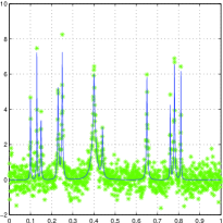
where we assume that ε𝝂subscript𝜀𝝂\varepsilon_{\mathchoice{\mbox{\boldmath$\displaystyle\nu$}}{\mbox{\boldmath$\textstyle\nu$}}{\mbox{\boldmath$\scriptstyle\nu$}}{\mbox{\boldmath$\scriptscriptstyle\nu$}}} are independently and normally distributed r.v. with 𝐄(εν)=0𝐄subscript𝜀𝜈0\mathbf{E}\left(\varepsilon_{\nu}\right)=0 and 𝐄(εν2)=σ2𝐄superscriptsubscript𝜀𝜈2superscript𝜎2\mathbf{E}\left(\varepsilon_{\nu}^{2}\right)=\sigma^{2}. The upper left image in Figure 2 depicts the true signal u0superscript𝑢0u^{0} (solid line) and the data Y𝑌Y, with m=1024𝑚1024m=1024 and σ=0.5𝜎0.5\sigma=0.5. The application we have in mind with this example arises in NMR spectroscopy, where the NMR spectra provide structural information on the number and type of chemical entities in a molecule. In this context, we suggest to choose J=TV2𝐽𝑇subscript𝑉2J=TV_{2}, since the true signal u0superscript𝑢0u^{0} is rather smooth (see [12] for examples where J𝐽J is chosen to be the total variation of the first and second derivative).

Finally, we discuss the MR-statistic T𝑇T in (4). We choose Λ=IdΛId\Lambda=\textnormal{Id} and the index set 𝒮𝒮\mathcal{S} to consist of all discrete intervals with side lengths ranging from 111 to 100100100. For an interval S𝒮𝑆𝒮S\in\mathcal{S} we set ωS=(#S)1/2χSsuperscript𝜔𝑆superscript#𝑆12subscript𝜒𝑆\omega^{S}=(\#S)^{-1/2}\chi_{S}. Thus, each SMRE solves the constrained optimization problem

infuUTV2(u) s.t. 1#S|𝝂S(Yu)𝝂|q(S𝒮).formulae-sequencesubscriptinfimum𝑢𝑈𝑇subscript𝑉2𝑢 s.t. 1#𝑆subscript𝝂𝑆subscript𝑌𝑢𝝂𝑞for-all𝑆𝒮\inf_{u\in U}TV_{2}(u)\quad\text{ s.t. }\quad\frac{1}{\sqrt{\#S}}\left|\sum_{\mathchoice{\mbox{\boldmath$\displaystyle\nu$}}{\mbox{\boldmath$\textstyle\nu$}}{\mbox{\boldmath$\scriptstyle\nu$}}{\mbox{\boldmath$\scriptscriptstyle\nu$}}\in S}(Y-u)_{\mathchoice{\mbox{\boldmath$\displaystyle\nu$}}{\mbox{\boldmath$\textstyle\nu$}}{\mbox{\boldmath$\scriptstyle\nu$}}{\mbox{\boldmath$\scriptscriptstyle\nu$}}}\right|\leq q\quad\forall(S\in\mathcal{S}). (22)

We choose q𝑞q to be the α𝛼\alpha-quantile of the MR-statistic T𝑇T, that is

qα=inf{q:(maxS𝒮1#S|𝝂Sε𝝂|q)α}α(0,1).formulae-sequencesubscript𝑞𝛼infimumconditional-set𝑞subscript𝑆𝒮1#𝑆subscript𝝂𝑆subscript𝜀𝝂𝑞𝛼𝛼01q_{\alpha}=\inf\left\{q\in\mathbb{R}~{}:~{}\mathbb{P}\left(\max_{S\in\mathcal{S}}\frac{1}{\sqrt{\#S}}\left|\sum_{\mathchoice{\mbox{\boldmath$\displaystyle\nu$}}{\mbox{\boldmath$\textstyle\nu$}}{\mbox{\boldmath$\scriptstyle\nu$}}{\mbox{\boldmath$\scriptscriptstyle\nu$}}\in S}\varepsilon_{\mathchoice{\mbox{\boldmath$\displaystyle\nu$}}{\mbox{\boldmath$\textstyle\nu$}}{\mbox{\boldmath$\scriptstyle\nu$}}{\mbox{\boldmath$\scriptscriptstyle\nu$}}}\right|\leq q\right)\geq\alpha\right\}\quad\alpha\in(0,1). (23)

We note that except for few special cases (cf. [28, 30]) closed form expressions for the distribution of the MT-statistic T𝑇T are usually not at hand. In practice one rather considers the empirical distribution of T𝑇T where the variance σ2superscript𝜎2\sigma^{2} can be estimated at a rate md𝑚𝑑\sqrt{md} (cf. [38]).

We will henceforth denote by u^αsubscript^𝑢𝛼\hat{u}_{\alpha} a solution of (22) with q=qα𝑞subscript𝑞𝛼q=q_{\alpha}. As argued in Section 1.1, u^αsubscript^𝑢𝛼\hat{u}_{\alpha} is smoother (i.e. has smaller value TV2𝑇subscript𝑉2TV_{2}) than the true signal u0superscript𝑢0u^{0} with a probability of at least α𝛼\alpha while it satisfies the constraint that the multiresolution statistic T𝑇T does not exceed qαsubscript𝑞𝛼q_{\alpha}. This is a sound statistical interpretation of the regularization parameter α𝛼\alpha.

Refer to caption
Refer to caption
Refer to caption
Refer to caption
Refer to caption
Refer to caption
Refer to caption
Refer to caption
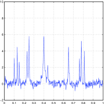
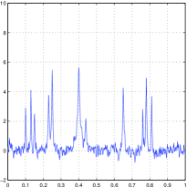
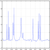
Figure 2. Row-wise from top left: true signal u0superscript𝑢0u^{0} (solid) with data Y𝑌Y, oracles u^L2subscript^𝑢superscriptL2\hat{u}_{\text{L}^{2}} and u^Bsubscript^𝑢B\hat{u}_{\text{B}}, AWS estimators u^awsTrianglesuperscriptsubscript^𝑢awsTriangle\hat{u}_{\text{aws}}^{\text{Triangle}} and u^awsGaussiansuperscriptsubscript^𝑢awsGaussian\hat{u}_{\text{aws}}^{\text{Gaussian}}, and the SMREs u^0.9subscript^𝑢0.9\hat{u}_{0.9}, u^0.75subscript^𝑢0.75\hat{u}_{0.75} and u^0.5subscript^𝑢0.5\hat{u}_{0.5}.

Numerical results and simulations.

In Figure 2 the oracles u^L2subscript^𝑢superscriptL2\hat{u}_{\text{L}^{2}} and u^Bsubscript^𝑢B\hat{u}_{\text{B}}, the AWS-estimators u^awsTrianglesuperscriptsubscript^𝑢awsTriangle\hat{u}_{\text{aws}}^{\text{Triangle}} and and u^awsGausssuperscriptsubscript^𝑢awsGauss\hat{u}_{\text{aws}}^{\text{Gauss}} as well as the SMRE u^0.9subscript^𝑢0.9\hat{u}_{0.9}, u^0.75subscript^𝑢0.75\hat{u}_{0.75} and u^0.5subscript^𝑢0.5\hat{u}_{0.5} are depicted. It is evident that the SMRE matches the smoothness of the true object much better than the other estimators while the essential features of the signal (such as peak location and peak height) are preserved. In particular, almost no additional local extrema are generated by our approach which stays in obvious contrast to the other methods. Moreover, we point out that the SMRE are quite robust w.r.t. the choice of the confidence level α𝛼\alpha.

We verify this behavior by a simulation study in Table 1. For different noise levels (σ=0.1,0.3𝜎0.10.3\sigma=0.1,0.3 and 0,5050,5) we compare the MISE, MIAE and MSB. Additionally, we compute the mean number of local maxima (MLM) of u^^𝑢\hat{u} relative to the number of local maxima in u0superscript𝑢0u^{0} (which is 111111). Here u^^𝑢\hat{u} is any of the above estimators. Note that the latter measure (similar to the MSB) takes into account the smoothness of the estimators where a value MLM1much-greater-thanMLM1\text{MLM}\gg 1 indicates too many local maxima and hence a lack of regularity whereas MLM<1MLM1\text{MLM}<1 implies severe oversmoothing.

σ=0.1𝜎0.1\sigma=0.1 σ=0.3𝜎0.3\sigma=0.3
MISE MSB MIAE MLM MISE MSB MIAE MLM
u^L2subscript^𝑢superscriptL2\hat{u}_{\text{L}^{2}} 0.009 0.008 0.071 11.881 0.046 0.027 0.156 10.915
u^Bsubscript^𝑢B\hat{u}_{\text{B}} 0.009 0.007 0.070 11.700 0.048 0.026 0.149 10.359
u^awsTrianglesuperscriptsubscript^𝑢awsTriangle\hat{u}_{\text{aws}}^{\text{Triangle}} 0.007 0.007 0.048 2.551 0.040 0.035 0.112 3.053
u^awsGausssuperscriptsubscript^𝑢awsGauss\hat{u}_{\text{aws}}^{\text{Gauss}} 0.054 0.040 0.068 1.971 0.062 0.041 0.107 2.230
u^0.9subscript^𝑢0.9\hat{u}_{0.9} 0.008 0.004 0.047 1.336 0.056 0.019 0.127 1.273
u^0.75subscript^𝑢0.75\hat{u}_{0.75} 0.007 0.004 0.044 1.342 0.050 0.018 0.121 1.290
u^0.5subscript^𝑢0.5\hat{u}_{0.5} 0.007 0.004 0.043 1.366 0.046 0.017 0.116 1.290
σ=0.5𝜎0.5\sigma=0.5
MISE MSB MIAE MLM
u^L2subscript^𝑢superscriptL2\hat{u}_{\text{L}^{2}} 0.091 0.037 0.213 9.860
u^Bsubscript^𝑢B\hat{u}_{\text{B}} 0.094 0.036 0.206 9.135
u^awsTrianglesuperscriptsubscript^𝑢awsTriangle\hat{u}_{\text{aws}}^{\text{Triangle}} 0.078 0.058 0.162 3.141
u^awsGausssuperscriptsubscript^𝑢awsGauss\hat{u}_{\text{aws}}^{\text{Gauss}} 0.079 0.043 0.149 2.330
u^0.9subscript^𝑢0.9\hat{u}_{0.9} 0.134 0.034 0.207 1.194
u^0.75subscript^𝑢0.75\hat{u}_{0.75} 0.120 0.032 0.196 1.241
u^0.5subscript^𝑢0.5\hat{u}_{0.5} 0.109 0.030 0.186 1.238
Table 1. Simulation studies for one dimensional peak data set.

As it becomes apparent from Table 1, the SMREs are performing similarly well when compared to the reference estimators as far as the standard measures MISE and MIAE are concerned. For small noise levels (σ=0.1𝜎0.1\sigma=0.1) SMREs even prove to be superior. The distance measures MSB and MLM, however, are significantly smaller for SMREs which indicates that these meet the smoothness of the true object u0superscript𝑢0u^{0} much better than the reference estimators (cf. Example 3.1 i)). All in all, the simulation results confirm our visual impressions above.

Implementation Details.

The current index set 𝒮𝒮\mathcal{S} results in an overall number of constraints in (22) of

#𝒮=i=1100(1024i+1)=97450.#𝒮superscriptsubscript𝑖11001024𝑖197450\#\mathcal{S}=\sum_{i=1}^{100}(1024-i+1)=97450.

As pointed out in Section 2.3, the efficiency of Dykstra’s Algorithm can be increased by grouping independent side-conditions, that is side-conditions corresponding to intervals in 𝒮𝒮\mathcal{S} with empty intersection. For example, the system 𝒮𝒮\mathcal{S} can be grouped such that the intersection of the corresponding sets D1,,DMsubscript𝐷1subscript𝐷𝑀D_{1},\ldots,D_{M} in (17) form 𝒞𝒞\mathcal{C} with

M=i=1100i=5050.𝑀superscriptsubscript𝑖1100𝑖5050M=\sum_{i=1}^{100}i=5050.

In all our simulations we set τ=104𝜏superscript104\tau=10^{-4} and λ=1.0𝜆1.0\lambda=1.0 in Algorithm 1 which results in k[τ]100𝑘delimited-[]𝜏100k[\tau]\approx 100 iterations and an overall computation time of approximately 202020 minutes for each SMRE. We note, however, that more than 95%percent9595\% of the computation time is needed for the projection step (12) and that a considerable speed up for the latter could be achieved by parallelization.

3.2. Image denoising

In this section we apply the SMRE technique to the problem of image denoising, that is non-parametric regression in d=2𝑑2d=2 dimensions. In other words, we consider the noise model (21) as in Section 3.1, where the index 𝝂𝝂\textstyle\nu ranges over the discrete square {1,,m}2superscript1𝑚2\left\{1,\ldots,m\right\}^{2}. In Figure 3 two typical examples for images u0superscript𝑢0u^{0} and noisy observations Y𝑌Y are depicted (m=512𝑚512m=512 and σ=0.1𝜎0.1\sigma=0.1, where u0superscript𝑢0u^{0} is scaled between 00 (black) and 111 (white)).

Refer to caption
Refer to caption
Refer to caption
Refer to caption
Figure 3. Standard test images “cameraman” (top) and “roof” (bottom) and their noisy counterparts.

We will use the total-variation semi-norm J=TV1β𝐽𝑇superscriptsubscript𝑉1𝛽J=TV_{1}^{\beta} as regularization functional (β=108𝛽superscript108\beta=10^{-8}). Moreover, we choose ΛΛ\Lambda to be defined as

Λ(v)𝝂=v𝝂2,(𝝂1,,m2).Λsubscript𝑣𝝂superscriptsubscript𝑣𝝂2for-all𝝂1superscript𝑚2\Lambda(v)_{\mathchoice{\mbox{\boldmath$\displaystyle\nu$}}{\mbox{\boldmath$\textstyle\nu$}}{\mbox{\boldmath$\scriptstyle\nu$}}{\mbox{\boldmath$\scriptscriptstyle\nu$}}}=v_{\mathchoice{\mbox{\boldmath$\displaystyle\nu$}}{\mbox{\boldmath$\textstyle\nu$}}{\mbox{\boldmath$\scriptstyle\nu$}}{\mbox{\boldmath$\scriptscriptstyle\nu$}}}^{2},\quad\forall(\mathchoice{\mbox{\boldmath$\displaystyle\nu$}}{\mbox{\boldmath$\textstyle\nu$}}{\mbox{\boldmath$\scriptstyle\nu$}}{\mbox{\boldmath$\scriptscriptstyle\nu$}}\in{1,\ldots,m}^{2}). (24)

The index set 𝒮𝒮\mathcal{S} is defined to be the collection of all discrete squares with side lengths ranging from 111 to 252525 and we set ωS=cSχSsuperscript𝜔𝑆subscript𝑐𝑆subscript𝜒𝑆\omega^{S}=c_{S}\chi_{S} with yet to be defined constants cSsubscript𝑐𝑆c_{S}. Thus, each SMREs solves the constrained optimization problem

infuUTV1β(u) s.t. 𝝂ScS(Yu)𝝂2q(S𝒮).formulae-sequencesubscriptinfimum𝑢𝑈𝑇superscriptsubscript𝑉1𝛽𝑢 s.t. subscript𝝂𝑆subscript𝑐𝑆superscriptsubscript𝑌𝑢𝝂2𝑞for-all𝑆𝒮\inf_{u\in U}TV_{1}^{\beta}(u)\quad\text{ s.t. }\quad\sum_{\mathchoice{\mbox{\boldmath$\displaystyle\nu$}}{\mbox{\boldmath$\textstyle\nu$}}{\mbox{\boldmath$\scriptstyle\nu$}}{\mbox{\boldmath$\scriptscriptstyle\nu$}}\in S}c_{S}(Y-u)_{\mathchoice{\mbox{\boldmath$\displaystyle\nu$}}{\mbox{\boldmath$\textstyle\nu$}}{\mbox{\boldmath$\scriptstyle\nu$}}{\mbox{\boldmath$\scriptscriptstyle\nu$}}}^{2}\leq q\quad\forall(S\in\mathcal{S}). (25)

We agree upon q=1𝑞1q=1 and specify the constants cSsubscript𝑐𝑆c_{S}. To this end, compute for s=1,,25𝑠125s=1,\ldots,25 the quantile values

qα,s=inf{q:(maxS𝒮#S=s𝝂Sε𝝂2q)1α}α(0,1)formulae-sequencesubscript𝑞𝛼𝑠infimumconditional-set𝑞subscript𝑆𝒮#𝑆𝑠subscript𝝂𝑆superscriptsubscript𝜀𝝂2𝑞1𝛼𝛼01q_{\alpha,s}=\inf\left\{q\in\mathbb{R}~{}:~{}\mathbb{P}\left(\max_{\begin{subarray}{c}S\in\mathcal{S}\\ \#S=s\end{subarray}}\sum_{\mathchoice{\mbox{\boldmath$\displaystyle\nu$}}{\mbox{\boldmath$\textstyle\nu$}}{\mbox{\boldmath$\scriptstyle\nu$}}{\mbox{\boldmath$\scriptscriptstyle\nu$}}\in S}\varepsilon_{\mathchoice{\mbox{\boldmath$\displaystyle\nu$}}{\mbox{\boldmath$\textstyle\nu$}}{\mbox{\boldmath$\scriptstyle\nu$}}{\mbox{\boldmath$\scriptscriptstyle\nu$}}}^{2}\leq q\right)\geq 1-\alpha\right\}\quad\alpha\in(0,1)

and set cS=qα,#S1subscript𝑐𝑆superscriptsubscript𝑞𝛼#𝑆1c_{S}=q_{\alpha,\#S}^{-1}. In other words, the definition of cSsubscript𝑐𝑆c_{S} implies that the true signal u0superscript𝑢0u^{0} satisfies the constraints in (25) for squares of a fixed side length s𝑠s with probability at least α𝛼\alpha. We will henceforth denote by u^αsubscript^𝑢𝛼\hat{u}_{\alpha} a solution of (25). We remark on this particular choice of the parameters ωSsubscript𝜔𝑆\omega_{S} below.

Numerical results and simulations.

In Figures 4 and 5 the oracles u^L2subscript^𝑢superscriptL2\hat{u}_{\text{L}^{2}} and u^Bsubscript^𝑢B\hat{u}_{\text{B}}, the AWS-estimators u^awsTrianglesuperscriptsubscript^𝑢awsTriangle\hat{u}_{\text{aws}}^{\text{Triangle}} and u^awsGausssuperscriptsubscript^𝑢awsGauss\hat{u}_{\text{aws}}^{\text{Gauss}} as well as the SMRE u^0.9subscript^𝑢0.9\hat{u}_{0.9} are depicted (for the “cameraman” and “roof” test image respectively). It is rather obvious that the L2superscriptL2\text{L}^{2}-oracles are not favorable: although relevant details in the image are preserved, smooth parts (as e.g. the sky) still contain random structures. In contrast, the estimator u^awsGausssuperscriptsubscript^𝑢awsGauss\hat{u}_{\text{aws}}^{\text{Gauss}} preserves smooth areas but looses essential details. The aws-estimator with triangular kernel performs much better, however, it gives piecewise constant reconstructions of smoothly varying portions of the image, which is clearly undesirable. The SMRE and the Bregman-oracle visually perform superior to the other methods. The good performance of the Bregman-oracle indicates that the symmetric Bregman distance is a good measure for comparing images. In contrast to the Bregman-oracle, the SMRE adapts the amount of smoothing to the underlying image structure: constant image areas are smoothed nicely (e.g. sky portions), while oscillating patterns (e.g. the grass part in the “cameraman” image or the roof tiles in the “roof” image) are recovered.

Refer to caption
Refer to caption
Refer to caption
Refer to caption
Refer to caption
Figure 4. Reconstructions “cameraman” (row-wise from top left): L2superscriptL2\text{L}^{2}-oracle u^L2subscript^𝑢superscriptL2\hat{u}_{\text{L}^{2}}, Bregman-oracle u^Bsubscript^𝑢𝐵\hat{u}_{B}, AWS estimators u^awsTrianglesuperscriptsubscript^𝑢awsTriangle\hat{u}_{\text{aws}}^{\text{Triangle}} and u^awsGaussiansuperscriptsubscript^𝑢awsGaussian\hat{u}_{\text{aws}}^{\text{Gaussian}}, and SMRE u^0.9subscript^𝑢0.9\hat{u}_{0.9}.
Refer to caption
Refer to caption
Refer to caption
Refer to caption
Refer to caption
Figure 5. Reconstructions “roof” (row-wise from top left): L2superscriptL2\text{L}^{2}-oracle u^L2subscript^𝑢superscriptL2\hat{u}_{\text{L}^{2}}, Bregman-oracle u^Bsubscript^𝑢𝐵\hat{u}_{B}, AWS estimators u^awsTrianglesuperscriptsubscript^𝑢awsTriangle\hat{u}_{\text{aws}}^{\text{Triangle}} and u^awsGaussiansuperscriptsubscript^𝑢awsGaussian\hat{u}_{\text{aws}}^{\text{Gaussian}}, and SMRE u^0.9subscript^𝑢0.9\hat{u}_{0.9}.

We evaluate the performance of the SMREs by means of a simulation study. To this end, we compute the MISE, MIAE and MSB and compare these values with the reference estimators. We note, however, that in particular the MISE and MIAE are not well suited in order to measure the distance of images for they are inconsistent with human eye perception. In [45] the structural similarity index (SSIM) was introduced for image quality assessment that takes into account luminance, contrast and structure of the images at the same time. We use the author’s implementation 333available at https://www.ece.uwaterloo.ca/~z70wang/research/ssim/ which is normalized such that the SSIM lies in the interval [1,1]11[-1,1] and is 111 in case of a perfect match. We denote by MSSIM the empirical mean of the SSIM in our simulations.

In Table 2 the simulation results are listed. A first striking fact is the good performance of the L2superscriptL2\text{L}^{2}-oracle w.r.t. the MISE and MIAE which is supposed to imply reconstruction properties superior to the other methods. Keeping in mind the visual comparison in Figures 4 and 5, however, this is rather questionable. On the other hand, it becomes evident that the L2superscriptL2\text{L}^{2}-oracle has a rather poor performance w.r.t. the MSB which is more suited for measuring image distances. It is therefore remarkable that the SMRE performs equally good as the Bregman-oracle which, in contrast to the SMRE, is not accessible (since u0superscript𝑢0u^{0} is usually unknown). As far as the structural similarity measure MSSIM is concerned our approach proves to be superior to all others. Finally, the simulation results indicate that aws estimation is not favourable for denoising of natural images.

“cameraman” “roof”
MISE MSB MIAE MSSIM MISE MSB MIAE MSSIM
u^L2subscript^𝑢superscriptL2\hat{u}_{\text{L}^{2}} 0.0017 0.0314 0.0276 0.7739 0.0029 0.0499 0.0383 0.6700
u^Bsubscript^𝑢B\hat{u}_{\text{B}} 0.0023 0.0256 0.0275 0.7995 0.0038 0.0405 0.0391 0.6607
u^awsTrianglesuperscriptsubscript^𝑢awsTriangle\hat{u}_{\text{aws}}^{\text{Triangle}} 0.0032 0.0482 0.0308 0.7657 0.0046 0.0702 0.0416 0.6205
u^awsGausssuperscriptsubscript^𝑢awsGauss\hat{u}_{\text{aws}}^{\text{Gauss}} 0.0046 0.0470 0.0360 0.7284 0.0053 0.0686 0.0457 0.5668
u^0.9subscript^𝑢0.9\hat{u}_{0.9} 0.0021 0.0252 0.0297 0.8024 0.0033 0.0374 0.0407 0.7003
Table 2. Simulation studies for the test images “cameraman” and “roof”.

Notes on the choice of ΛΛ\Lambda and ωSsuperscript𝜔𝑆\omega^{S}.

In general, a proper choice of the transformation ΛΛ\Lambda and of the weight-functions ωSsuperscript𝜔𝑆\omega^{S} can be achieved by including prior structural information on the true image to be estimated. Substantial parts of natural images, such as photographs, consists of oscillating patterns (as e.g. fabric, wood, hair, grass etc.). This becomes obvious in the standard test images depicted in Figure 3. We claim that for signals that exhibit oscillating patterns, a quadratic transformation ΛΛ\Lambda as in (24) is favorable, since it yields (compared to the linear statistic studied in Section 3.1) a larger power of the local test statistic on small scales.

In order to illustrate this, we simulate noisy observations Y𝑌Y of the test images u𝑢u in Figure 3 as in (21) with σ=0.1𝜎0.1\sigma=0.1 and compute a global estimator u^^𝑢\hat{u} by computing a minimizer of the ROF-functional (20) (with λ=0.1𝜆0.1\lambda=0.1). We intend to examine how well over-smoothed regions in u^^𝑢\hat{u} are detected by the MR-statistic T(Yu^)𝑇𝑌^𝑢T(Y-\hat{u}) as in (4) with two different average functions (cf. (5))

μ1,S(v)=|𝝂Svν| and μ2,S(v)=𝝂Svν2formulae-sequencesubscript𝜇1𝑆𝑣subscript𝝂𝑆subscript𝑣𝜈 and subscript𝜇2𝑆𝑣subscript𝝂𝑆superscriptsubscript𝑣𝜈2\mu_{1,S}(v)=\left|\sum_{\mathchoice{\mbox{\boldmath$\displaystyle\nu$}}{\mbox{\boldmath$\textstyle\nu$}}{\mbox{\boldmath$\scriptstyle\nu$}}{\mbox{\boldmath$\scriptscriptstyle\nu$}}\in S}v_{\nu}\right|\quad\text{ and }\quad\mu_{2,S}(v)=\sum_{\mathchoice{\mbox{\boldmath$\displaystyle\nu$}}{\mbox{\boldmath$\textstyle\nu$}}{\mbox{\boldmath$\scriptstyle\nu$}}{\mbox{\boldmath$\scriptscriptstyle\nu$}}\in S}v_{\nu}^{2}

respectively. For the sake of simplicity we restrict for the moment our considerations on the index set 𝒮𝒮\mathcal{S} of all 5×5555\times 5 sub-squares in {1,,m}2superscript1𝑚2\left\{1,\ldots,m\right\}^{2}. In Figure 6 the local means μi,Ssubscript𝜇𝑖𝑆\mu_{i,S} of the residuals v=Yu^𝑣𝑌^𝑢v=Y-\hat{u} for the “roof”-image are depicted. To be more precise, the center coordinate of each square S𝒮𝑆𝒮S\in\mathcal{S} is colored according to μi,Ssubscript𝜇𝑖𝑆\mu_{i,S}, Hence, large values indicate locations where the estimator u^^𝑢\hat{u} is considered over-smoothed according to the statistic. It becomes visually clear that the localization of oversmoothed regions is better for μ2,Ssubscript𝜇2𝑆\mu_{2,S}. This is a good motivation for incorporating the local means of the squared residuals in the SMRE model (7).
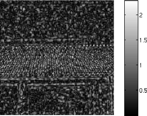
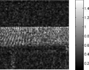
Refer to caption
Refer to caption
Figure 6. Local means μ1,Ssubscript𝜇1𝑆\mu_{1,S} (left) and μ2,Ssubscript𝜇2𝑆\mu_{2,S} (right)) of the residuals for “roof” image.

We finally comment on the choice of cSsubscript𝑐𝑆c_{S}. Since ε𝝂subscript𝜀𝝂\varepsilon_{\mathchoice{\mbox{\boldmath$\displaystyle\nu$}}{\mbox{\boldmath$\textstyle\nu$}}{\mbox{\boldmath$\scriptstyle\nu$}}{\mbox{\boldmath$\scriptscriptstyle\nu$}}} are independent and normally distributed random variables, the (scaled) average function

σ2μS(ε)=𝝂S(ε𝝂σ)2superscript𝜎2subscript𝜇𝑆𝜀subscript𝝂𝑆superscriptsubscript𝜀𝝂𝜎2\sigma^{-2}\mu_{S}(\varepsilon)=\sum_{\mathchoice{\mbox{\boldmath$\displaystyle\nu$}}{\mbox{\boldmath$\textstyle\nu$}}{\mbox{\boldmath$\scriptstyle\nu$}}{\mbox{\boldmath$\scriptscriptstyle\nu$}}\in S}\left(\frac{\varepsilon_{\mathchoice{\mbox{\boldmath$\displaystyle\nu$}}{\mbox{\boldmath$\textstyle\nu$}}{\mbox{\boldmath$\scriptstyle\nu$}}{\mbox{\boldmath$\scriptscriptstyle\nu$}}}}{\sigma}\right)^{2}

is χ2superscript𝜒2\chi^{2} distributed with #S#𝑆\#S degrees of freedom. Note that the distribution of σ2μS(ε)superscript𝜎2subscript𝜇𝑆𝜀\sigma^{-2}\mu_{S}(\varepsilon) is identical only for sets S𝑆S of the same scale #S#𝑆\#S. As a consequence of this, it is likely that certain scales dominate the supremum in the MR-statistic T𝑇T which spoils the multiscale properties of our approach. As a way out, we compute normalizing constants for each scale separately.

An alternative approach would be to search for transformations that turn μS(ε)subscript𝜇𝑆𝜀\mu_{S}(\varepsilon) into almost identically distributed random variables. Logarithmic and p𝑝p-root transformations are often employed for this purpose (see e.g. [25]). This will be investigated separately.

Implementation Details.

The current index set 𝒮𝒮\mathcal{S} results in an overall number of constraints in (25) of

#𝒮=i=125(512i+1)2=6251300.#𝒮superscriptsubscript𝑖125superscript512𝑖126251300\#\mathcal{S}=\sum_{i=1}^{25}(512-i+1)^{2}=6251300.

Again by grouping independent side-conditions, the system 𝒮𝒮\mathcal{S} can be grouped such that the intersection of the corresponding sets D1,,DMsubscript𝐷1subscript𝐷𝑀D_{1},\ldots,D_{M} in (17) form 𝒞𝒞\mathcal{C} with

M=i=125i2=5525.𝑀superscriptsubscript𝑖125superscript𝑖25525M=\sum_{i=1}^{25}i^{2}=5525.

In all our simulations we set τ=104𝜏superscript104\tau=10^{-4} and λ=0.25𝜆0.25\lambda=0.25 in Algorithm 1 which results in k[τ]30𝑘delimited-[]𝜏30k[\tau]\approx 30 iterations and a overall computation time of approximately 222 hours for each SMRE. Hence, parallelization is clearly desirable in this case.

3.3. Deconvolution

Another interesting class of problems which can be approached by means of SMREs are deconvolution problems. To be more precise, we assume that K𝐾K is a convolution operator, that is

(Ku)𝝂=(ku)𝝂=𝒎dk𝝂𝒎u𝒎subscript𝐾𝑢𝝂subscript𝑘𝑢𝝂subscript𝒎superscript𝑑subscript𝑘𝝂𝒎subscript𝑢𝒎(Ku)_{\mathchoice{\mbox{\boldmath$\displaystyle\nu$}}{\mbox{\boldmath$\textstyle\nu$}}{\mbox{\boldmath$\scriptstyle\nu$}}{\mbox{\boldmath$\scriptscriptstyle\nu$}}}=(k\ast u)_{\mathchoice{\mbox{\boldmath$\displaystyle\nu$}}{\mbox{\boldmath$\textstyle\nu$}}{\mbox{\boldmath$\scriptstyle\nu$}}{\mbox{\boldmath$\scriptscriptstyle\nu$}}}=\sum_{\mathchoice{\mbox{\boldmath$\displaystyle m$}}{\mbox{\boldmath$\textstyle m$}}{\mbox{\boldmath$\scriptstyle m$}}{\mbox{\boldmath$\scriptscriptstyle m$}}\in\mathbb{R}^{d}}k_{\mathchoice{\mbox{\boldmath$\displaystyle\nu$}}{\mbox{\boldmath$\textstyle\nu$}}{\mbox{\boldmath$\scriptstyle\nu$}}{\mbox{\boldmath$\scriptscriptstyle\nu$}}-\mathchoice{\mbox{\boldmath$\displaystyle m$}}{\mbox{\boldmath$\textstyle m$}}{\mbox{\boldmath$\scriptstyle m$}}{\mbox{\boldmath$\scriptscriptstyle m$}}}u_{\mathchoice{\mbox{\boldmath$\displaystyle m$}}{\mbox{\boldmath$\textstyle m$}}{\mbox{\boldmath$\scriptstyle m$}}{\mbox{\boldmath$\scriptscriptstyle m$}}}

where k𝑘k is a square-summable kernel on the lattice dsuperscript𝑑\mathbb{Z}^{d} and uH𝑢𝐻u\in H is extended by zero-padding. We will focus on the situation where k𝑘k is a circular Gaussian kernel with standard deviation σ𝜎\sigma given by

k𝝂=1(2πσ)dei=1dνi22σ2.subscript𝑘𝝂1superscript2𝜋𝜎𝑑superscript𝑒superscriptsubscript𝑖1𝑑superscriptsubscript𝜈𝑖22superscript𝜎2k_{\mathchoice{\mbox{\boldmath$\displaystyle\nu$}}{\mbox{\boldmath$\textstyle\nu$}}{\mbox{\boldmath$\scriptstyle\nu$}}{\mbox{\boldmath$\scriptscriptstyle\nu$}}}=\frac{1}{(\sqrt{2\pi}\sigma)^{d}}e^{-\frac{\sum_{i=1}^{d}\nu_{i}^{2}}{2\sigma^{2}}}. (26)

With Z=Y+λpk1+vk𝑍𝑌𝜆subscript𝑝𝑘1subscript𝑣𝑘Z=Y+\lambda p_{k-1}+v_{k}, the primal step (13) in Algorithm 1 amounts to solve

ukargminuH12𝝂X((Ku)𝝂Z𝝂)2+λJ(u),subscript𝑢𝑘subscriptargmin𝑢𝐻12subscript𝝂𝑋superscriptsubscript𝐾𝑢𝝂subscript𝑍𝝂2𝜆𝐽𝑢u_{k}\leftarrow\operatorname*{\textnormal{argmin}}_{u\in H}\frac{1}{2}\sum_{\mathchoice{\mbox{\boldmath$\displaystyle\nu$}}{\mbox{\boldmath$\textstyle\nu$}}{\mbox{\boldmath$\scriptstyle\nu$}}{\mbox{\boldmath$\scriptscriptstyle\nu$}}\in X}((Ku)_{\mathchoice{\mbox{\boldmath$\displaystyle\nu$}}{\mbox{\boldmath$\textstyle\nu$}}{\mbox{\boldmath$\scriptstyle\nu$}}{\mbox{\boldmath$\scriptscriptstyle\nu$}}}-Z_{\mathchoice{\mbox{\boldmath$\displaystyle\nu$}}{\mbox{\boldmath$\textstyle\nu$}}{\mbox{\boldmath$\scriptstyle\nu$}}{\mbox{\boldmath$\scriptscriptstyle\nu$}}})^{2}+\lambda J(u),

where we choose J𝐽J to be as in (18) and apply the techniques described in [44] for the numerical solution.

In order to illustrate the performance of our approach in practical applications, we give an example from confocal microscopy, nowadays a standard technique in fluorescence microscopy (cf. [39]). When recording images with this kind of microscope, the original object gets blurred by a Gaussian kernel (in first order). The observations (photon counts) can be modeled as a Poisson process, i.e.

Y𝝂=Poiss((Ku0)𝝂),𝝂X.formulae-sequencesubscript𝑌𝝂Poisssubscript𝐾superscript𝑢0𝝂𝝂𝑋Y_{\mathchoice{\mbox{\boldmath$\displaystyle\nu$}}{\mbox{\boldmath$\textstyle\nu$}}{\mbox{\boldmath$\scriptstyle\nu$}}{\mbox{\boldmath$\scriptscriptstyle\nu$}}}=\text{Poiss}((Ku^{0})_{\mathchoice{\mbox{\boldmath$\displaystyle\nu$}}{\mbox{\boldmath$\textstyle\nu$}}{\mbox{\boldmath$\scriptstyle\nu$}}{\mbox{\boldmath$\scriptscriptstyle\nu$}}}),\quad\mathchoice{\mbox{\boldmath$\displaystyle\nu$}}{\mbox{\boldmath$\textstyle\nu$}}{\mbox{\boldmath$\scriptstyle\nu$}}{\mbox{\boldmath$\scriptscriptstyle\nu$}}\in X. (27)

The image depicted in Figure 7(a) shows a recording of a PtK2 cell taken from the kidney of potorous tridactylus. Before the recording, the protein β𝛽\beta-tubulin was tagged with a fluorescent marker such that it can be traced by the microscope. The image in 7(a) shows an area of 18×18181818\times 18 \tcmum2\tcmusuperscriptm2\tcmu\text{m}^{2} at a resolution of 798×798798798798\times 798 pixel. The point spread function of the optical system can be modeled as a Gaussian kernel with full width at half maximum of 230230230nm, which corresponds to σ=4.3422𝜎4.3422\sigma=4.3422 in (26).

Note that (27) does not fall immediately into the range of models covered by (1). We will adapt the present situation to the SMRE methodology described in Section 1 by standardization and consider instead of (3) the modified problem

infuUJ(u) s.t.T(YKuKu)1subscriptinfimum𝑢𝑈𝐽𝑢 s.t.𝑇𝑌𝐾𝑢𝐾𝑢1\inf_{u\in U}J(u)\quad\text{ s.t.}\quad T\left(\frac{Y-Ku}{\sqrt{Ku}}\right)\leq 1 (28)

where the division is understood pointwise. Clearly, the problem of finding a solution of (28) is much more involved than solving (3) for the constraints being nonconvex: firstly, the functional G𝐺G as defined in (9) is nonconvex as a consequence of which the convergence result in Theorem 2.2 does not apply and secondly Dykstra’s projection algorithm as described in Section 2 cannot be employed.

We propose the following ansatz in order to circumvent this problem: instead of projecting onto the intersection 𝒞𝒞\mathcal{C} of sets CSsubscript𝐶𝑆C_{S} as described in (15), we now project in the k𝑘k-th step of Algorithm 1 onto

𝒞P[k]=n=1NCP,S[k]whereCP,S[k]={vH:μS(v/Kuk)q}.formulae-sequencesubscript𝒞𝑃delimited-[]𝑘superscriptsubscript𝑛1𝑁subscript𝐶𝑃𝑆delimited-[]𝑘wheresubscript𝐶𝑃𝑆delimited-[]𝑘conditional-set𝑣𝐻subscript𝜇𝑆𝑣𝐾subscript𝑢𝑘𝑞\mathcal{C}_{P}[k]=\bigcap_{n=1}^{N}C_{P,S}[k]\quad\text{where}\quad C_{P,S}[k]=\left\{v\in H~{}:~{}\mu_{S}\left(v/\sqrt{Ku_{k}}\right)\leq q\right\}.

with a pointwise division by the square root of Kuk𝐾subscript𝑢𝑘Ku_{k}. Put differently, in the k𝑘k-th step of Algorithm 1 we use the previous estimate uksubscript𝑢𝑘u_{k} of u0superscript𝑢0u^{0} as a lagged standardization in order to approximate the constraints in (28). In fact, we use max(Kuk,ε)𝐾subscript𝑢𝑘𝜀\sqrt{\max(Ku_{k},\varepsilon)} with a small number ε>0𝜀0\varepsilon>0 for standardization, in order to avoid instabilities.

We note that while with this modification Dykstra’s algorithm becomes applicable again, the projection problem (12) now changes in each iteration step of Algorithm 1. As a consequence, Theorem 2.2 does not hold anymore after this modification, either. So far, we have not come up with a similar convergence analysis.

We compute the SMRE u^0.9subscript^𝑢0.9\hat{u}_{0.9} by employing Algorithm 1 with the modifications described above. As in the denoising examples in Section 3.2 the index set 𝒮𝒮\mathcal{S} consists of all squares with the side-lengths {1,,25}125\left\{1,\ldots,25\right\} and we choose ωS=χSsuperscript𝜔𝑆subscript𝜒𝑆\omega^{S}=\chi_{S} and Λ=IdΛId\Lambda=\textnormal{Id}. We note, that this results in an overall number of #𝒮=95436200#𝒮95436200\#\mathcal{S}=95~{}436~{}200 inequality constraints. The constant q𝑞q are chosen as in (23), where we assume that ε𝝂subscript𝜀𝝂\varepsilon_{\mathchoice{\mbox{\boldmath$\displaystyle\nu$}}{\mbox{\boldmath$\textstyle\nu$}}{\mbox{\boldmath$\scriptstyle\nu$}}{\mbox{\boldmath$\scriptscriptstyle\nu$}}} are independent and standard normally distributed r.v.

In Algorithm 1 we set λ=0.05𝜆0.05\lambda=0.05 and compute 100100100 steps. We observe that after a few iterations (15similar-toabsent15\sim 15) the error τ𝜏\tau falls below 103superscript10310^{-3} and almost stagnates thereafter, which is due to the fact that we do not increase the accuracy in the subroutines for (13) and (12). Each iteration step in Algorithm 1 approximately takes 101010 minutes, where 90%percent9090\% of the computation time is needed for (13). The result is depicted in Figure 7(b).
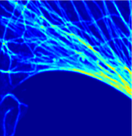
Refer to caption
(a) Fluorescence microscopy data of a PtK2 cell in potorous tridactylus kidney. The bright filaments indicate the location of the protein β𝛽\beta-tubulin.
Refer to caption
(b) SMRE u^0.9subscript^𝑢0.9\hat{u}_{0.9}: fully automated and locally adaptive deconvolution of microscopy data.
Figure 7. Reconstruction of confocal microscopy data.

The benefits of our method are twofold:

  1. i)

    The amount of regularization is chosen in a completely automatic way. The only parameter to be selected is the level α𝛼\alpha in (23). Note that the parameter λ𝜆\lambda in Algorithm 1 has no effect on the output (though it has an effect on the number of iterations needed and the numerical stability).

  2. ii)

    The reconstruction has an appealing locally adaptive behavior which in the present example mainly concerns the gaps between the protein filaments: whereas the marked β𝛽\beta-tubulin is concentrated in regions of basically one scale, the gaps in between actually make up the multiscale nature of the image.
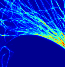
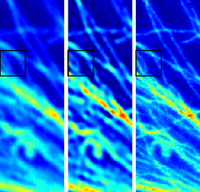
Refer to caption
(a) STED microscopy recording of the PtK2 cell data set.
Refer to caption
(b) Detail comparison between confocal recording (left), SMRE u^0.9subscript^𝑢0.9\hat{u}_{0.9} (middle) and STED recording (right).
Figure 8. Comparison with high-resolution STED microscopy data.

In the present situation we are in the comfortable position to have a reference image at hand by means of which we can evaluate the result of our method: STED (STimulated Emission Depletion) microscopy constitutes a relatively new method, that is capable of recording images at a physically 555-101010 times higher resolution as confocal microscopy (see [27, 26]). Hence a STED image of this object may serve as “gold standard” reference image.

Figure 8(a) depicts a STED recording of the PtK2 cell data set in Figure 7(a). The comparison of the SMRE u^0.9subscript^𝑢0.9\hat{u}_{0.9} with the STED recording in Figure 8(b) shows that our SMRE technique chooses a reasonable amount of regularization: no artifacts due to under-regularization are generated and on the other hand almost all relevant geometrical features that are present in the high-resolution STED recording become visible in the reconstruction. In particular, we note that filament bifurcations (one such bifurcation is marked by a black box in Figure 8(b)) become apparent in our reconstruction that are not visible in the recorded data.

Finally, we mention that aside to standardization, other transformations of the Poisson data (27) could possibly be considered. For example Anscombe’s transformation is known to yield reasonable approximations to normality even for low Poisson-intensities and hence has a particular appeal for e.g. microscopy data with low photon-counts. We are currently investigating SMREs that employ Anscombe’s transform, where in particular the arising projection problems are challenging.

4. Conclusion and Outlook

In this work, we propose a general estimation technique for nonparametric inverse regression problems in the white noise model (1) based on the convex program (7). It amounts to finding a minimizer of a convex regularization functional J(u)𝐽𝑢J(u) over a set of feasible estimators that satisfy the fidelty condition T(YKu)q𝑇𝑌𝐾𝑢𝑞T(Y-Ku)\leq q, where T𝑇T is assumed to be the maximum over simple convex constraints and q𝑞q is some quantile of the statistic T(ε)𝑇𝜀T(\varepsilon). Any such minimizer we call statistical multiresolution estimator (SMRE). This approach covers well known uni-scale techniques, such as the Dantzig selector, but with a vast field of potentially new application areas, such as locally adaptive imaging. The particular appeal of the multi-scale generalization arises for those situations where a “neighboring relationship” within the signal can be employed to gain additional information by “averaging” neighboring residuals. We demonstrate in various examples that this improvement is drastic.

We approach the numerical solution of the problem by the ADMM (cf. Algorithm 1) that decomposes the problem into two subproblems: A J𝐽J-penalized least squares problem, independent of T𝑇T, and an orthogonal projection problem onto the feasible set of (7) that is independent of J𝐽J. The first problem is well studied and for most typical choices of J𝐽J fast and reliable numerical approaches are at hand. The projection problem, however, is computational demanding, in particular for image denoising applications. We propose Dykstra’s cyclic projection method for its approximate solution. Finally, by extensive numerical experiments, we illustrate the performance of our estimation scheme (in nonparametric regression, image denoising and deblurring problems) and the applicability of our algorithmic approach.

Summarizing, this paper is meant to introduce a novel class of statistical estimators, to provide a general algorithmic approach for their numerical computation and to evaluate their performance by numerical simulations. The inherent questions on the asymptotic behaviour of these estimators (such as consistency, convergence rates or oracle inequalities) remain —to a large extent— unanswered. This opens an interesting area for future research.

A first attempt has been made in [21] where it is assumed that the model space Uu0superscript𝑢0𝑈U\ni u^{0} is some Hilbert-space of real valued functions on some domain ΩΩ\Omega and that K:UL2(Ω):𝐾𝑈superscriptL2ΩK:U\rightarrow\text{L}^{2}(\Omega) is linear and bounded. The error model (1) then has to be adapted accordingly. When Y𝑌Y is a Gaussian process on L2(Ω)superscriptL2Ω\text{L}^{2}(\Omega) with mean Ku0𝐾superscript𝑢0Ku^{0} and variance σ2>0superscript𝜎20\sigma^{2}>0, consistency and convergence rates for SMREs as σ0+𝜎superscript0\sigma\rightarrow 0^{+} have been proved in [21] for the case when Λ=IdΛId\Lambda=\textnormal{Id}. However, in order to extend these results to the present setting, one would rather work with a discrete sample of Ku0𝐾subscript𝑢0Ku_{0} on the grid X𝑋X and then consider the case when the number of observations N=md𝑁𝑚𝑑N=md tends to infinity. The previous analysis in [21] indicates two major aspects that have to be considered in the asymptotic analysis for SMREs:

  1. (a)

    As N𝑁N\rightarrow\infty usually the cardinality of the index set 𝒮𝒮\mathcal{S} (and hence of the set of weight functions 𝒲𝒲\mathcal{W}) gets unbounded. Thus, the mutliresolution statistic T(ε)=TN(ε)𝑇𝜀subscript𝑇𝑁𝜀T(\varepsilon)=T_{N}(\varepsilon) in (4) is likely to degenerate unless it is properly normalized and 𝒲𝒲\mathcal{W} satisfies some entropy condition. In the linear case (Λ=IdΛId\Lambda=\textnormal{Id}) we utilized a result from [17] that guarantees a.s. boundedness of TN(ε)subscript𝑇𝑁𝜀T_{N}(\varepsilon).

  2. (b)

    In order to derive convergence rates (or risk bounds) it is well known that the true signal u0superscript𝑢0u^{0} has to satisfy some apriori regularity conditions. When using general convex regularization functionals J𝐽J, this is usually expressed by the source condition

    Kp0J(u0), for some p0L2(Ω).formulae-sequencesuperscript𝐾superscript𝑝0𝐽superscript𝑢0 for some superscript𝑝0superscriptL2ΩK^{*}p^{0}\in\partial J(u^{0}),\text{ for some }p^{0}\in\text{L}^{2}(\Omega).

    Here Ksuperscript𝐾K^{*} denotes the adjoint of K𝐾K and J𝐽\partial J the (generalized) derivative of J𝐽J. For example, if J(u)=12u2𝐽𝑢12superscriptnorm𝑢2J(u)=\frac{1}{2}\left\|u\right\|^{2}, then this conditions means that u0ran(K)superscript𝑢0ransuperscript𝐾u^{0}\in\textnormal{ran}(K^{*}).

It would be of great interest to transfer and extend the results in [21] to the present situation. It is to be expected that (a) and (a) above are necessary assumptions for this purpose.

As stressed by the referees, other extensions are of interest and will be postponed to future work. In contrast to imaging, in many other applications the design X𝑋X is random, rather than fixed. In these situations an obvious way to extend our algorithmic framework would be to select suitable partitions 𝒮𝒮\mathcal{S} according to the design density, i.e. with finer resolution at locations with a high concentration of design points. It also remains an open issue how to extend the SMRE methodology to density estimation rather than regression, in particular in a deconvolution setup. For d=1𝑑1d=1 a first step in this direction has been taken in [11] and it will be of great interest to explore whether our approach allow this to be extended to d2𝑑2d\geq 2.

Acknowledgement

K.F. and A.M. are supported by the DFG-SNF Research Group FOR916 Statistical Regularization and Qualitative constraints. P.M is supported by the BMBF project 030303MUPAH666 INVERS. A.M and P.M. are supported by the SFB755 Photonic Imaging on the Nanoscale and the SFB803 Functionality Controlled by Organization in and between Membranes.

We thank S. Hell, A. Egner and A. Schoenle (Department of NanoBiophotonics, Max Planck Institute for Biophysical Chemistry, Göttingen) for providing the microscopy data and L. Dümbgen (University of Bern) for stimulating discussions. Finally, we are grateful to an associate editor and to an anonymous referee for their helpful comments.

Appendix A Proofs

In this section we shall give the proofs of Theorems 2.2 and 2.4 as well as Corollary 2.5. We note, that convergence of Algorithm 1 is a classical subject in optimization theory and a proof can e.g. be found in [20, Chap. III Thm. 4.1]. However, in order to apply these results, it is necessary that certain regularity conditions for J𝐽J hold, that are not realistic for our purposes (as e.g. in the case of total-variation regularization). The assertions of Theorems 2.2 and 2.4 are modifications of the standard results.

Moreover, we will allow for approximate solution of the subproblems (12) and (13). To this end, we rewrite these two subproblems as variational inequalities, i.e. given (uk1,vk1,pk1)subscript𝑢𝑘1subscript𝑣𝑘1subscript𝑝𝑘1(u_{k-1},v_{k-1},p_{k-1}) we find (uk,vk,pk)subscript𝑢𝑘subscript𝑣𝑘subscript𝑝𝑘(u_{k},v_{k},p_{k}) such that

G(v)G(vk)+λ1Kuk1+vkYλpk1,vvkεk,vHformulae-sequence𝐺𝑣𝐺subscript𝑣𝑘superscript𝜆1𝐾subscript𝑢𝑘1subscript𝑣𝑘𝑌𝜆subscript𝑝𝑘1𝑣subscript𝑣𝑘subscript𝜀𝑘for-all𝑣𝐻\displaystyle G(v)-G(v_{k})+\lambda^{-1}\left\langle Ku_{k-1}+v_{k}-Y-\lambda p_{k-1},v-v_{k}\right\rangle\geq-\varepsilon_{k},\;\forall v\in H (29a)
J(u)J(uk)+λ1Kuk+vkYλpk1,KuKukδk,uUformulae-sequence𝐽𝑢𝐽subscript𝑢𝑘superscript𝜆1𝐾subscript𝑢𝑘subscript𝑣𝑘𝑌𝜆subscript𝑝𝑘1𝐾𝑢𝐾subscript𝑢𝑘subscript𝛿𝑘for-all𝑢𝑈\displaystyle J(u)-J(u_{k})+\lambda^{-1}\left\langle Ku_{k}+v_{k}-Y-\lambda p_{k-1},Ku-Ku_{k}\right\rangle\geq-\delta_{k},\;\forall u\in U (29b)
pk=pk1(Kuk+vkY)/λ,subscript𝑝𝑘subscript𝑝𝑘1𝐾subscript𝑢𝑘subscript𝑣𝑘𝑌𝜆\displaystyle p_{k}=p_{k-1}-(Ku_{k}+v_{k}-Y)/\lambda, (29c)

where we assume that {ε1,ε2,}subscript𝜀1subscript𝜀2\left\{\varepsilon_{1},\varepsilon_{2},\ldots\right\} and {δ1,δ2,}subscript𝛿1subscript𝛿2\left\{\delta_{1},\delta_{2},\ldots\right\} are given sequences of positive numbers. Note that (29a) implies that G(vk)=0𝐺subscript𝑣𝑘0G(v_{k})=0 and hence vk𝒞subscript𝑣𝑘𝒞v_{k}\in\mathcal{C} and that for εk=δk=0subscript𝜀𝑘subscript𝛿𝑘0\varepsilon_{k}=\delta_{k}=0 (29a) and (29b) are equivalent to (12) and (13), respectively.

Finally, we remind the reader of the definition of the subdifferential (or generalized derivative) F𝐹\partial F of a convex function F:V:𝐹𝑉F:V\rightarrow\mathbb{R} on a real Hilbert-space V𝑉V:

ξF(v)F(w)F(v)+ξ,wvV(wV).formulae-sequence𝜉𝐹𝑣𝐹𝑤𝐹𝑣subscript𝜉𝑤𝑣𝑉for-all𝑤𝑉\xi\in\partial F(v)\quad\Leftrightarrow\quad F(w)\geq F(v)+\left\langle\xi,w-v\right\rangle_{V}\;\forall(w\in V).

If ξF(v)𝜉𝐹𝑣\xi\in\partial F(v), then ξ𝜉\xi is called subgradient of F𝐹F at v𝑣v. It follows from [19, Chap III, Prop. 3.1 and Prop. 4.1] that the Lagrangian L𝐿L (and hence also the augmented Lagrangian Lλsubscript𝐿𝜆L_{\lambda}) has a saddle-point (u^,v^,p^)U×H×H^𝑢^𝑣^𝑝𝑈𝐻𝐻(\hat{u},\hat{v},\hat{p})\in U\times H\times H if and only if

Ku^+v^=Y,Kp^J(u^) and p^G(v^).formulae-sequence𝐾^𝑢^𝑣𝑌formulae-sequencesuperscript𝐾^𝑝𝐽^𝑢 and ^𝑝𝐺^𝑣K\hat{u}+\hat{v}=Y,\quad K^{*}\hat{p}\in\partial J(\hat{u})\quad\text{ and }\quad\hat{p}\in\partial G(\hat{v}). (30)

We will henceforth assume that {(uk,vk,pk)}ksubscriptsubscript𝑢𝑘subscript𝑣𝑘subscript𝑝𝑘𝑘\left\{(u_{k},v_{k},p_{k})\right\}_{k\in\mathbb{N}} is a sequence generated by iteratively repeating the steps (29a) - (29c). Further, we introduce the notation

u¯k:=uku^,v¯k:=vkv^ and p¯k:=pkp^.formulae-sequenceassignsubscript¯𝑢𝑘subscript𝑢𝑘^𝑢formulae-sequenceassignsubscript¯𝑣𝑘subscript𝑣𝑘^𝑣 and assignsubscript¯𝑝𝑘subscript𝑝𝑘^𝑝\bar{u}_{k}:=u_{k}-\hat{u},\quad\bar{v}_{k}:=v_{k}-\hat{v}\quad\text{ and }\quad\bar{p}_{k}:=p_{k}-\hat{p}.

We start with the following

Lemma A.1.

For all k1𝑘1k\geq 1 we have that

(p¯k12+λ2Ku¯k12)(p¯k2+λ2Ku¯k2)λ2(Ku¯k+v¯k2+Ku¯k1Ku¯k2)2λ2(δk+δk1)δkεksuperscriptdelimited-∥∥subscript¯𝑝𝑘12superscript𝜆2superscriptdelimited-∥∥𝐾subscript¯𝑢𝑘12superscriptdelimited-∥∥subscript¯𝑝𝑘2superscript𝜆2superscriptdelimited-∥∥𝐾subscript¯𝑢𝑘2superscript𝜆2superscriptdelimited-∥∥𝐾subscript¯𝑢𝑘subscript¯𝑣𝑘2superscriptdelimited-∥∥𝐾subscript¯𝑢𝑘1𝐾subscript¯𝑢𝑘22superscript𝜆2subscript𝛿𝑘subscript𝛿𝑘1subscript𝛿𝑘subscript𝜀𝑘\left(\left\|\bar{p}_{k-1}\right\|^{2}+\lambda^{-2}\left\|K\bar{u}_{k-1}\right\|^{2}\right)-\left(\left\|\bar{p}_{k}\right\|^{2}+\lambda^{-2}\left\|K\bar{u}_{k}\right\|^{2}\right)\\ \geq\lambda^{-2}\left(\left\|K\bar{u}_{k}+\bar{v}_{k}\right\|^{2}+\left\|K\bar{u}_{k-1}-K\bar{u}_{k}\right\|^{2}\right)-2\lambda^{-2}(\delta_{k}+\delta_{k-1})-\delta_{k}-\varepsilon_{k} (31)
Proof.

The assertion follows by repeating the steps (5.6)-(5.25) in the proof of [20, Chap. III Thm. 4.1] after replacing (5.9) and (5.10) by (29a) and (29b) respectively. ∎

We continue with the proof of Theorem 2.2. More precisely, we prove the following generalized version

Proposition A.2.

Assume that the sums k=1δksuperscriptsubscript𝑘1subscript𝛿𝑘\sum_{k=1}^{\infty}\delta_{k} and k=1εksuperscriptsubscript𝑘1subscript𝜀𝑘\sum_{k=1}^{\infty}\varepsilon_{k} are finite. Then, the sequence {(uk,vk)}k1subscriptsubscript𝑢𝑘subscript𝑣𝑘𝑘1\left\{(u_{k},v_{k})\right\}_{k\geq 1} is bounded in U×H𝑈𝐻U\times H and every weak cluster point is a solution of (8). Moreover,

kKuk+vkY2+K(ukuk1)2<.subscript𝑘superscriptnorm𝐾subscript𝑢𝑘subscript𝑣𝑘𝑌2superscriptnorm𝐾subscript𝑢𝑘subscript𝑢𝑘12\sum_{k\in\mathbb{N}}\left\|Ku_{k}+v_{k}-Y\right\|^{2}+\left\|K(u_{k}-u_{k-1})\right\|^{2}<\infty.
Proof.

Let k1𝑘1k\geq 1 and define D=k=1δk𝐷superscriptsubscript𝑘1subscript𝛿𝑘D=\sum_{k=1}^{\infty}\delta_{k} and E=k=1εk𝐸superscriptsubscript𝑘1subscript𝜀𝑘E=\sum_{k=1}^{\infty}\varepsilon_{k}. Summing up Inequality (31) over k𝑘k and keeping in mind that Ku¯k+v¯k=Kuk+vkY𝐾subscript¯𝑢𝑘subscript¯𝑣𝑘𝐾subscript𝑢𝑘subscript𝑣𝑘𝑌K\bar{u}_{k}+\bar{v}_{k}=Ku_{k}+v_{k}-Y and Ku¯k1Ku¯k=Kuk1Kuk𝐾subscript¯𝑢𝑘1𝐾subscript¯𝑢𝑘𝐾subscript𝑢𝑘1𝐾subscript𝑢𝑘K\bar{u}_{k-1}-K\bar{u}_{k}=Ku_{k-1}-Ku_{k} shows

k=1Kuk+vkY2+Kuk1Kuk2λ2p^2+Ku^2+(4λ2+1)D+E<superscriptsubscript𝑘1superscriptdelimited-∥∥𝐾subscript𝑢𝑘subscript𝑣𝑘𝑌2superscriptdelimited-∥∥𝐾subscript𝑢𝑘1𝐾subscript𝑢𝑘2superscript𝜆2superscriptdelimited-∥∥^𝑝2superscriptdelimited-∥∥𝐾^𝑢24superscript𝜆21𝐷𝐸\sum_{k=1}^{\infty}\left\|Ku_{k}+v_{k}-Y\right\|^{2}+\left\|Ku_{k-1}-Ku_{k}\right\|^{2}\\ \leq\lambda^{2}\left\|\hat{p}\right\|^{2}+\left\|K\hat{u}\right\|^{2}+(4\lambda^{-2}+1)D+E<\infty

where we have used that u¯0=u^subscript¯𝑢0^𝑢\bar{u}_{0}=\hat{u} and p¯0=p^subscript¯𝑝0^𝑝\bar{p}_{0}=\hat{p}. Furthermore, it follows again from (31) that

p¯k2+λ2Ku¯2p^2+λ2Ku^2+(4λ2+1)D+E<superscriptnormsubscript¯𝑝𝑘2superscript𝜆2superscriptnorm𝐾¯𝑢2superscriptnorm^𝑝2superscript𝜆2superscriptnorm𝐾^𝑢24superscript𝜆21𝐷𝐸\left\|\bar{p}_{k}\right\|^{2}+\lambda^{-2}\left\|K\bar{u}\right\|^{2}\leq\left\|\hat{p}\right\|^{2}+\lambda^{-2}\left\|K\hat{u}\right\|^{2}+(4\lambda^{-2}+1)D+E<\infty (32)

This together with the fact that Kuk+vkY0norm𝐾subscript𝑢𝑘subscript𝑣𝑘𝑌0\left\|Ku_{k}+v_{k}-Y\right\|\rightarrow 0 shows that

max(Kuk,vk,pk)=𝒪(1).norm𝐾subscript𝑢𝑘normsubscript𝑣𝑘normsubscript𝑝𝑘𝒪1\max(\left\|Ku_{k}\right\|,\left\|v_{k}\right\|,\left\|p_{k}\right\|)=\mathcal{O}(1).

Together with the optimality condition for (13) this in turn implies that for an arbitrary uH𝑢𝐻u\in H

J(uk)J(u)+λ1Kuk+vkYλpk1,KuKuk+δk=𝒪(1).𝐽subscript𝑢𝑘𝐽𝑢superscript𝜆1𝐾subscript𝑢𝑘subscript𝑣𝑘𝑌𝜆subscript𝑝𝑘1𝐾𝑢𝐾subscript𝑢𝑘subscript𝛿𝑘𝒪1J(u_{k})\leq J(u)+\lambda^{-1}\left\langle Ku_{k}+v_{k}-Y-\lambda p_{k-1},Ku-Ku_{k}\right\rangle+\delta_{k}=\mathcal{O}(1). (33)

Summarizing, we find that

maxS𝒮μS(KukY)+J(uk)maxS𝒮ωSΛ(KukY)+J(uk)c<subscript𝑆𝒮subscript𝜇𝑆𝐾subscript𝑢𝑘𝑌𝐽subscript𝑢𝑘subscript𝑆𝒮normsuperscript𝜔𝑆normΛ𝐾subscript𝑢𝑘𝑌𝐽subscript𝑢𝑘𝑐\max_{S\in\mathcal{S}}\mu_{S}(Ku_{k}-Y)+J(u_{k})\leq\max_{S\in\mathcal{S}}\left\|\omega^{S}\right\|\left\|\Lambda(Ku_{k}-Y)\right\|+J(u_{k})\leq c<\infty

for a suitably chosen constant c𝑐c\in\mathbb{R}, since ΛΛ\Lambda is supposed to be continuous. Thus, it follows from Assumption A that {uk}ksubscriptsubscript𝑢𝑘𝑘\left\{u_{k}\right\}_{k\in\mathbb{N}} is bounded and hence sequentially weakly compact. Now, let (u~,v~,p~)~𝑢~𝑣~𝑝(\tilde{u},\tilde{v},\tilde{p}) be a weak cluster point of {(uk,vk,pk)}ksubscriptsubscript𝑢𝑘subscript𝑣𝑘subscript𝑝𝑘𝑘\left\{(u_{k},v_{k},p_{k})\right\}_{k\in\mathbb{N}} and recall that (u^,v^,p^)^𝑢^𝑣^𝑝(\hat{u},\hat{v},\hat{p}) was assumed to be a saddle point of the augmented Lagrangian Lλsubscript𝐿𝜆L_{\lambda}. Setting u=u^𝑢^𝑢u=\hat{u} in (33) thus results in

J(uk)J(u^)+λ1Kuk+vkY,Ku^Kuk+pk1,KukKu^+δk=J(u^)+pk1,KukKu^+o(1)𝐽subscript𝑢𝑘𝐽^𝑢superscript𝜆1𝐾subscript𝑢𝑘subscript𝑣𝑘𝑌𝐾^𝑢𝐾subscript𝑢𝑘subscript𝑝𝑘1𝐾subscript𝑢𝑘𝐾^𝑢subscript𝛿𝑘𝐽^𝑢subscript𝑝𝑘1𝐾subscript𝑢𝑘𝐾^𝑢o1\begin{split}J(u_{k})&\leq J(\hat{u})+\lambda^{-1}\left\langle Ku_{k}+v_{k}-Y,K\hat{u}-Ku_{k}\right\rangle+\left\langle p_{k-1},Ku_{k}-K\hat{u}\right\rangle+\delta_{k}\\ &=J(\hat{u})+\left\langle p_{k-1},Ku_{k}-K\hat{u}\right\rangle+\text{o}(1)\end{split} (34)

Using the relation Ku^+v^=Y𝐾^𝑢^𝑣𝑌K\hat{u}+\hat{v}=Y we further find

pk1,KukKu^=pk1,KukY+v^=pk1,Kuk+vkYpk1,vkv^=o(1)pk1,vkv^subscript𝑝𝑘1𝐾subscript𝑢𝑘𝐾^𝑢subscript𝑝𝑘1𝐾subscript𝑢𝑘𝑌^𝑣subscript𝑝𝑘1𝐾subscript𝑢𝑘subscript𝑣𝑘𝑌subscript𝑝𝑘1subscript𝑣𝑘^𝑣o1subscript𝑝𝑘1subscript𝑣𝑘^𝑣\left\langle p_{k-1},Ku_{k}-K\hat{u}\right\rangle=\left\langle p_{k-1},Ku_{k}-Y+\hat{v}\right\rangle\\ =\left\langle p_{k-1},Ku_{k}+v_{k}-Y\right\rangle-\left\langle p_{k-1},v_{k}-\hat{v}\right\rangle=\text{o}(1)-\left\langle p_{k-1},v_{k}-\hat{v}\right\rangle (35)

From the definition of vksubscript𝑣𝑘v_{k} in (29a) and from the fact that v^,vk𝒞^𝑣subscript𝑣𝑘𝒞\hat{v},v_{k}\in\mathcal{C} it follows that

Y+λpk1(Kuk1+vk),v^vkεk𝑌𝜆subscript𝑝𝑘1𝐾subscript𝑢𝑘1subscript𝑣𝑘^𝑣subscript𝑣𝑘subscript𝜀𝑘\left\langle Y+\lambda p_{k-1}-(Ku_{k-1}+v_{k}),\hat{v}-v_{k}\right\rangle\leq\varepsilon_{k}

which in turn implies that

pk1,vkv^λ1Y(Kuk1+vk),vkv^+εk=λ1Y(Kuk+vk),vkv^+λ1KukKuk1,vkv^+εk=o(1)subscript𝑝𝑘1subscript𝑣𝑘^𝑣superscript𝜆1𝑌𝐾subscript𝑢𝑘1subscript𝑣𝑘subscript𝑣𝑘^𝑣subscript𝜀𝑘superscript𝜆1𝑌𝐾subscript𝑢𝑘subscript𝑣𝑘subscript𝑣𝑘^𝑣superscript𝜆1𝐾subscript𝑢𝑘𝐾subscript𝑢𝑘1subscript𝑣𝑘^𝑣subscript𝜀𝑘o1-\left\langle p_{k-1},v_{k}-\hat{v}\right\rangle\leq\lambda^{-1}\left\langle Y-(Ku_{k-1}+v_{k}),v_{k}-\hat{v}\right\rangle+\varepsilon_{k}\\ =\lambda^{-1}\left\langle Y-(Ku_{k}+v_{k}),v_{k}-\hat{v}\right\rangle+\lambda^{-1}\left\langle Ku_{k}-Ku_{k-1},v_{k}-\hat{v}\right\rangle+\varepsilon_{k}=\text{o}(1) (36)

Combining (34), (35) and (36) gives

lim supkJ(uk)J(u^).subscriptlimit-supremum𝑘𝐽subscript𝑢𝑘𝐽^𝑢\limsup_{k\rightarrow\infty}J(u_{k})\leq J(\hat{u}).

Now, choose a subsequence {uρ(k)}ksubscriptsubscript𝑢𝜌𝑘𝑘\left\{u_{\rho(k)}\right\}_{k\in\mathbb{N}} such that uρ(k)u~subscript𝑢𝜌𝑘~𝑢u_{\rho(k)}\rightharpoonup\tilde{u}. Since J𝐽J is convex and lower semi-continuous it is also weakly lower semi-continuous and hence the previous estimate yields

J(u~)lim infkJ(uρ(k))J(u^).𝐽~𝑢subscriptlimit-infimum𝑘𝐽subscript𝑢𝜌𝑘𝐽^𝑢J(\tilde{u})\leq\liminf_{k\rightarrow\infty}J(u_{\rho(k)})\leq J(\hat{u}).

Moreover, we have that vρ(k)𝒞subscript𝑣𝜌𝑘𝒞v_{\rho(k)}\in\mathcal{C} for all k𝑘k\in\mathbb{N}. Since 𝒞𝒞\mathcal{C} is closed we conclude that v^𝒞^𝑣𝒞\hat{v}\in\mathcal{C}. Since Ku~+v~=Y𝐾~𝑢~𝑣𝑌K\tilde{u}+\tilde{v}=Y this shows that (u~,v~)~𝑢~𝑣(\tilde{u},\tilde{v}) solves (8) and thus J(u~)=J(u^)𝐽~𝑢𝐽^𝑢J(\tilde{u})=J(\hat{u}). ∎

We proceed with the proof of Theorem 2.4. Again we present a generalized version. To this end, let D𝐷D and E𝐸E be as in Proposition A.2.

Proposition A.3.

There exists a constant C=C(λ,u^,v^,p^,E,D)𝐶𝐶𝜆^𝑢^𝑣^𝑝𝐸𝐷C=C(\lambda,\hat{u},\hat{v},\hat{p},E,D) such that

0J(u[τ])J(u^)Kp^,u[τ]u^UCτ+δk[τ]+εk[τ](τ>0).formulae-sequence0𝐽𝑢delimited-[]𝜏𝐽^𝑢subscriptsuperscript𝐾^𝑝𝑢delimited-[]𝜏^𝑢𝑈𝐶𝜏subscript𝛿𝑘delimited-[]𝜏subscript𝜀𝑘delimited-[]𝜏for-all𝜏00\leq J(u[\tau])-J(\hat{u})-\left\langle K^{*}\hat{p},u[\tau]-\hat{u}\right\rangle_{U}\leq C\tau+\delta_{k[\tau]}+\varepsilon_{k[\tau]}\quad\forall(\tau>0).
Proof.

Define B2=(4λ1+1)D+Esuperscript𝐵24superscript𝜆11𝐷𝐸B^{2}=(4\lambda^{-1}+1)D+E. Then it follows from (32) that

λ1KukKu^p^+λ1Ku^+Bsuperscript𝜆1norm𝐾subscript𝑢𝑘𝐾^𝑢norm^𝑝superscript𝜆1norm𝐾^𝑢𝐵\displaystyle\lambda^{-1}\left\|Ku_{k}-K\hat{u}\right\|\leq\left\|\hat{p}\right\|+\lambda^{-1}\left\|K\hat{u}\right\|+B (37)
pk2p^+λ1Ku^+B,normsubscript𝑝𝑘2norm^𝑝superscript𝜆1norm𝐾^𝑢𝐵\displaystyle\left\|p_{k}\right\|\leq 2\left\|\hat{p}\right\|+\lambda^{-1}\left\|K\hat{u}\right\|+B, (38)

where (u^,v^,p^)^𝑢^𝑣^𝑝(\hat{u},\hat{v},\hat{p}) is an arbitrary saddle point of Lλ(u,v,p)subscript𝐿𝜆𝑢𝑣𝑝L_{\lambda}(u,v,p). Assume that τ>0𝜏0\tau>0 and that k=k[τ]𝑘𝑘delimited-[]𝜏k=k[\tau] is such that

max(Kuk+vkY,Kuk1Kuk)τ.norm𝐾subscript𝑢𝑘subscript𝑣𝑘𝑌norm𝐾subscript𝑢𝑘1𝐾subscript𝑢𝑘𝜏\max(\left\|Ku_{k}+v_{k}-Y\right\|,\left\|Ku_{k-1}-Ku_{k}\right\|)\leq\tau.

Then, it follows from (34), (36), (37) and (38) and that

J(uk)J(u^)+λ1Kuk+vkY,Ku^Kuk+pk1,KukKu^+δkJ(u^)+τ(p^+λ1Ku^+B)+pk1τ+pk1,v^vk+δkJ(u^)+τ(3p^+2λ1Ku^+2B)+2λ1τvkv^+δk+εk𝐽subscript𝑢𝑘𝐽^𝑢superscript𝜆1𝐾subscript𝑢𝑘subscript𝑣𝑘𝑌𝐾^𝑢𝐾subscript𝑢𝑘subscript𝑝𝑘1𝐾subscript𝑢𝑘𝐾^𝑢subscript𝛿𝑘𝐽^𝑢𝜏delimited-∥∥^𝑝superscript𝜆1delimited-∥∥𝐾^𝑢𝐵delimited-∥∥subscript𝑝𝑘1𝜏subscript𝑝𝑘1^𝑣subscript𝑣𝑘subscript𝛿𝑘𝐽^𝑢𝜏3delimited-∥∥^𝑝2superscript𝜆1delimited-∥∥𝐾^𝑢2𝐵2superscript𝜆1𝜏delimited-∥∥subscript𝑣𝑘^𝑣subscript𝛿𝑘subscript𝜀𝑘\begin{split}J(u_{k})&\leq J(\hat{u})+\lambda^{-1}\left\langle Ku_{k}+v_{k}-Y,K\hat{u}-Ku_{k}\right\rangle+\left\langle p_{k-1},Ku_{k}-K\hat{u}\right\rangle+\delta_{k}\\ &\leq J(\hat{u})+\tau(\left\|\hat{p}\right\|+\lambda^{-1}\left\|K\hat{u}\right\|+B)+\left\|p_{k-1}\right\|\tau+\left\langle p_{k-1},\hat{v}-v_{k}\right\rangle+\delta_{k}\\ &\leq J(\hat{u})+\tau(3\left\|\hat{p}\right\|+2\lambda^{-1}\left\|K\hat{u}\right\|+2B)+2\lambda^{-1}\tau\left\|v_{k}-\hat{v}\right\|+\delta_{k}+\varepsilon_{k}\end{split} (39)

After observing that KukKu^+vkv^=Y𝐾subscript𝑢𝑘𝐾^𝑢subscript𝑣𝑘^𝑣𝑌Ku_{k}-K\hat{u}+v_{k}-\hat{v}=Y it follows that vkv^τ+KukKu^normsubscript𝑣𝑘^𝑣𝜏norm𝐾subscript𝑢𝑘𝐾^𝑢\left\|v_{k}-\hat{v}\right\|\leq\tau+\left\|Ku_{k}-K\hat{u}\right\| and combining (39) and (37) gives

J(uk)J(u^)+τ(5p^+4λ1Ku^+4B+2λ1τ)+δk+εk.𝐽subscript𝑢𝑘𝐽^𝑢𝜏5norm^𝑝4superscript𝜆1norm𝐾^𝑢4𝐵2superscript𝜆1𝜏subscript𝛿𝑘subscript𝜀𝑘J(u_{k})\leq J(\hat{u})+\tau\left(5\left\|\hat{p}\right\|+4\lambda^{-1}\left\|K\hat{u}\right\|+4B+2\lambda^{-1}\tau\right)+\delta_{k}+\varepsilon_{k}.

Now, observe that from the definition of the subgradient and (30), it follows that J(uk)J(u^)+Kp^,uku^𝐽subscript𝑢𝑘𝐽^𝑢superscript𝐾^𝑝subscript𝑢𝑘^𝑢J(u_{k})\geq J(\hat{u})+\left\langle K^{*}\hat{p},u_{k}-\hat{u}\right\rangle and that p^,vkv^0^𝑝subscript𝑣𝑘^𝑣0\left\langle\hat{p},v_{k}-\hat{v}\right\rangle\leq 0. This and the fact that Ku^+v^=Y𝐾^𝑢^𝑣𝑌K\hat{u}+\hat{v}=Y implies that

0J(uk)J(u^)Kp^,uku^=J(uk)J(u^)p^,Kuk+vkY+p^,Ku^+v^Y+p^,vkv^J(uk)J(u^)+p^ττ(6p^+4λ1Ku^+4B+2λ1τ)+δk+εk.0𝐽subscript𝑢𝑘𝐽^𝑢superscript𝐾^𝑝subscript𝑢𝑘^𝑢𝐽subscript𝑢𝑘𝐽^𝑢^𝑝𝐾subscript𝑢𝑘subscript𝑣𝑘𝑌^𝑝𝐾^𝑢^𝑣𝑌^𝑝subscript𝑣𝑘^𝑣𝐽subscript𝑢𝑘𝐽^𝑢delimited-∥∥^𝑝𝜏𝜏6delimited-∥∥^𝑝4superscript𝜆1delimited-∥∥𝐾^𝑢4𝐵2superscript𝜆1𝜏subscript𝛿𝑘subscript𝜀𝑘\begin{split}0&\leq J(u_{k})-J(\hat{u})-\left\langle K^{*}\hat{p},u_{k}-\hat{u}\right\rangle\\ &=J(u_{k})-J(\hat{u})-\left\langle\hat{p},Ku_{k}+v_{k}-Y\right\rangle+\left\langle\hat{p},K\hat{u}+\hat{v}-Y\right\rangle+\left\langle\hat{p},v_{k}-\hat{v}\right\rangle\\ &\leq J(u_{k})-J(\hat{u})+\left\|\hat{p}\right\|\tau\\ &\leq\tau\left(6\left\|\hat{p}\right\|+4\lambda^{-1}\left\|K\hat{u}\right\|+4B+2\lambda^{-1}\tau\right)+\delta_{k}+\varepsilon_{k}.\end{split} (40)

This together with (39) finally proves the first part of the assertion. ∎

Remark A.4.

For the case when D=E=0𝐷𝐸0D=E=0, it is seen from the proof of Proposition (A.3) that the constant C𝐶C takes the simple form

C=τ(6p^+4Ku^+2τλ).𝐶𝜏6norm^𝑝4norm𝐾^𝑢2𝜏𝜆C=\tau\left(6\left\|\hat{p}\right\|+\frac{4\left\|K\hat{u}\right\|+2\tau}{\lambda}\right).
Proof of Corollary 2.5.

Assume that J(u)=12LuV2𝐽𝑢12subscriptsuperscriptnorm𝐿𝑢2𝑉J(u)=\frac{1}{2}\left\|Lu\right\|^{2}_{V}. Then it follows (see e.g. [22, Lem. 2.4]) that the subdifferential J(u^)𝐽^𝑢\partial J(\hat{u}) consists of the single element LLu^superscript𝐿𝐿^𝑢L^{*}L\hat{u}. Hence the extremality relations (30) imply that Kp^=LLu^superscript𝐾^𝑝superscript𝐿𝐿^𝑢K^{*}\hat{p}=L^{*}L\hat{u}. Now it is easy to observe that

J(uk)J(u^)Kp^,uku^=12L(uku^)V2.𝐽subscript𝑢𝑘𝐽^𝑢superscript𝐾^𝑝subscript𝑢𝑘^𝑢12subscriptsuperscriptnorm𝐿subscript𝑢𝑘^𝑢2𝑉J(u_{k})-J(\hat{u})-\left\langle K^{*}\hat{p},u_{k}-\hat{u}\right\rangle=\frac{1}{2}\left\|L(u_{k}-\hat{u})\right\|^{2}_{V}.

References

  • [1] J.-F. Aujol, G. Aubert, L. Blanc-Féraud, and A. Chambolle. Image decomposition into a bounded variation component and an oscillating component. J. Math. Imaging Vision, 22(1):71–88, 2005.
  • [2] S. Becker, E. Candès, and M. Grant. Templates for convex cone problems with applications to sparse signal recovery. Math. Program. Comput., 3:165–218, 2011.
  • [3] M. Bertalmio, V. Caselles, B. Rougé, and A. Solé. TV based image restoration with local constraints. J. Sci. Comput., 19(1-3):95–122, 2003. Special issue in honor of the sixtieth birthday of Stanley Osher.
  • [4] P. J. Bickel, Y. Ritov, and A. B. Tsybakov. Simultaneous analysis of lasso and Dantzig selector. Ann. Statist., 37(4):1705–1732, 2009.
  • [5] J. P. Boyle and R. L. Dykstra. A method for finding projections onto the intersection of convex sets in Hilbert spaces. In Advances in order restricted statistical inference (Iowa City, Iowa, 1985), volume 37 of Lecture Notes in Statist., pages 28–47. Springer, Berlin, 1986.
  • [6] L. Boysen, A. Kempe, V. Liebscher, A. Munk, and O. Wittich. Consistencies and rates of convergence of jump-penalized least squares estimators. Ann. Statist., 37(1):157–183, 2009.
  • [7] E. Candès and T. Tao. The Dantzig selector: statistical estimation when p𝑝p is much larger than n𝑛n. Ann. Statist., 35(6):2313–2351, 2007.
  • [8] S. S. Chen, D. L. Donoho, and M. A. Saunders. Atomic decomposition by basis pursuit. SIAM Review, 43(1):129–159, 2001.
  • [9] I. Csiszár. Why least squares and maximum entropy? An axiomatic approach to inference for linear inverse problems. Ann. Statist., 19(4):2032–2066, 1991.
  • [10] P. L. Davies and A. Kovac. Local extremes, runs, strings and multiresolution. Ann. Statist., 29(1):1–65, 2001. With discussion and rejoinder by the authors.
  • [11] P. L. Davies and A. Kovac. Densities, spectral densities and modality. Ann. Statist., 32(3):1093–1136, 2004.
  • [12] P. L. Davies, A. Kovac, and M. Meise. Nonparametric regression, confidence regions and regularization. Ann. Statist., 37(5B):2597–2625, 2009.
  • [13] F. Deutsch and H. Hundal. The rate of convergence of Dykstra’s cyclic projections algorithm: the polyhedral case. Numer. Funct. Anal. Optim., 15(5-6):537–565, 1994.
  • [14] D. C. Dobson and C. R. Vogel. Convergence of an iterative method for total variation denoising. SIAM J. Numer. Anal., 34(5):1779–1791, 1997.
  • [15] Y. Dong, M. Hintermüller, and M. Rincon-Camacho. Automated regularization parameter selection in multi-scale total variation models for image restoration. J. Math. Imaging Vision, 40:82–104(23), May 2011.
  • [16] L. Dümbgen and R. B. Johns. Confidence bands for isotonic median curves using sign tests. J. Comput. Graph. Statist, 13(2):519–533, 2004.
  • [17] L. Dümbgen and V. G. Spokoiny. Multiscale testing of qualitative hypotheses. Ann. Statist., 29(1):124–152, 2001.
  • [18] L. Dümbgen and G. Walther. Multiscale inference about a density. Ann. Statist., 36(4):1758–1785, 2008.
  • [19] I. Ekeland and R. Temam. Convex analysis and variational problems, volume 1 of Studies in Mathematics and its Applications. North-Holland Publishing Co., Amsterdam-Oxford, 1976.
  • [20] M. Fortin and R. Glowinski. Augmented Lagrangian methods, volume 15 of Studies in Mathematics and its Applications. North-Holland Publishing Co., Amsterdam, 1983. Applications to the numerical solution of boundary value problems, Translated from the French by B. Hunt and D. C. Spicer.
  • [21] K. Frick, P. Marnitz, and A. Munk. Shape constrained regularisation by statistical multiresolution for inverse problems: Asymptotic analysis. Technical report, 2010. Available at http://arxiv.org/abs/1003.3323.
  • [22] K. Frick and O. Scherzer. Regularization of ill-posed linear equations by the non-stationary Augmented Lagrangian Method. J. Integral Equations Appl., 22(2):217–257, 2010.
  • [23] N. Gaffke and R. Mathar. A cyclic projection algorithm via duality. Metrika, 36:29–54, 1989.
  • [24] M. Grasmair. The equivalence of the taut string algorithm and BV-regularization. J. Math. Imaging Vision, 27(1):59–66, 2007.
  • [25] D. M. Hawkins and R. Wixley. A note on the transformation of chi-squared variables to normality. Amer.Statist., 40(4):296–298, 1986.
  • [26] S. W. Hell. Far-Field Optical Nanoscopy. Science, 316(5828):1153–1158, 2007.
  • [27] S. W. Hell and J. Wichmann. Breaking the diffraction resolution limit by stimulated emission: stimulated-emission-depletion fluorescence microscopy. Opt. Lett., 19(11):780–782, 1994.
  • [28] T. Hotz, P. Marnitz, R. Stichtenoth, L. Davies, Z. Kabluchko, and A. Munk. Locally adaptive image denoising by a statistical multiresolution criterion. Comput. Stat. Data An., 56(3):543 – 558, 2012.
  • [29] G. M. James, P. Radchenko, and J. Lv. Dasso: connections between the dantzig selector and lasso. J. R. Stat. Soc. Ser. B Stat. Methodol., 71:127–142, 2009.
  • [30] Z. Kabluchko. Extremes of the standardized Gaussian noise. Stochastic Process. Appl., 121(3):515–533, 2011.
  • [31] Z. Kabluchko and A. Munk. Shao’s theorem on the maximum of standardized random walk increments for multidimensional arrays. ESAIM Probab. Stat., 13:409–416, 2009.
  • [32] J. Kaipio and E. Somersalo. Statistical and computational inverse problems, volume 160 of Applied Mathematical Sciences. Springer-Verlag, New York, 2005.
  • [33] Z. Lu, T. K. Pong, and Y. Zhang. An alternating direction method for finding Dantzig selectors. Technical report, 2010. Available at http://arxiv.org/abs/1011.4604v1.
  • [34] E. Mammen and S. van de Geer. Locally adaptive regression splines. Ann. Statist., 25(1):387–413, 1997.
  • [35] Y. Meyer. Oscillating patterns in image processing and nonlinear evolution equations, volume 22 of University Lecture Series. American Mathematical Society, Providence, RI, 2001. The fifteenth Dean Jacqueline B. Lewis memorial lectures.
  • [36] T. Mildenberger. A geometric interpretation of the multiresolution criterion in nonparametric regression. J. Nonparametr. Stat., 20(7):1048–5252, 2008.
  • [37] G. O. Mohler, A. L. Bertozzi, T. A. Goldstein, and S. J. Osher. Fast TV regularization for 2d maximum penalized likelihood estimation. J. Comput. Graph. Statist, 20(2):479–491, 2011.
  • [38] A. Munk, N. Bissantz, T. Wagner, and G. Freitag. On difference-based variance estimation in nonparametric regression when the covariate is high dimensional. J. R. Stat. Soc. Ser. B Stat. Methodol., 67(1):19–41, 2005.
  • [39] J. B. Pawley. Handbook of Biological Confocal Microscopy. Springer, 2006.
  • [40] J. Polzehl and V. G. Spokoiny. Adaptive weights smoothing with applications to image restoration. J. R. Stat. Soc. Ser. B Stat. Methodol., 62(2):335–354, 2000.
  • [41] J. K. Romberg. The dantzig selector and generalized thresholding. In CISS, pages 22–25. IEEE, 2008.
  • [42] D. Siegmund and B. Yakir. Tail probabilities for the null distribution of scanning statistics. Bernoulli, 6(2):191–213, 2000.
  • [43] R. Tibshirani. Regression shrinkage and selection via the lasso. J. R. Stat. Soc. Ser. B Stat. Methodol., 58:267–288, 1994.
  • [44] C. R. Vogel. Computational methods for inverse problems, volume 23 of Frontiers in Applied Mathematics. Society for Industrial and Applied Mathematics (SIAM), Philadelphia, PA, 2002. With a foreword by H. T. Banks.
  • [45] Z. Wang, A. C. Bovik, H. R. Sheikh, and E. P. Simoncelli. Image quality assessment: From error visibility to structural similarity. IEEE Trans. Image Process., 13(4):600–612, 2004.
  • [46] S. Xu. Estimation of the convergence rate of Dykstra’s cyclic projections algorithm in polyhedral case. Acta Math. Appl. Sinica (English Ser.), 16(2):217–220, 2000.