Peak Reduction and Clipping Mitigation by Compressive Sensing

Abstract

This work establishes the design, analysis, and fine-tuning of a Peak-to-Average-Power-Ratio (PAPR) reducing system, based on compressed sensing at the receiver of a peak-reducing sparse clipper applied to an OFDM signal at the transmitter. By exploiting the sparsity of the OFDM signal in the time domain relative to a pre-defined clipping threshold, the method depends on partially observing the frequency content of extremely simple sparse clippers to recover the locations, magnitudes, and phases of the clipped coefficients of the peak-reduced signal. We claim that in the absence of optimization algorithms at the transmitter that confine the frequency support of clippers to a predefined set of reserved-tones, no other tone-reservation method can reliably recover the original OFDM signal with such low complexity.

Afterwards we focus on designing different clipping signals that can embed a priori information regarding the support and phase of the peak-reducing signal to the receiver, followed by modified compressive sensing techniques for enhanced recovery. This includes data-based weighted $\ell_{1}$ minimization for enhanced support recovery and phase-augmention for homogeneous clippers followed by Bayesian techniques.

We show that using such techniques for a typical OFDM signal of 256 subcarriers and 20$\%$ reserved tones, the PAPR can be reduced by approximately 4.5 dB with a significant increase in capacity compared to a system which uses all its tones for data transmission and clips to such levels. The design is hence appealing from both capacity and PAPR reduction aspects.

I Introduction

Despite the introduction of Single Carrier Frequency Division Multiple Access (SC-FDMA) into current multicarrier transmission standards, the success of Orthogonal Frequency Division Multiplexing (OFDM) in high data rate transmission remains truly remarkable, with no better proof than the fact that variants of the IEEE 802.16 and IEEE 802.18 standards are still emerging [1, 2].

The main problem with OFDM signalling however lies in the high temporal peaks relative to the signal mean, portrayed in a parameter most commonly referred to as Peak-to-Average-Power-Ratio (PAPR). Since an OFDM signal is typically constructed by the superposition of a large number of modulated subcarriers, its envelope fluctuates with significant variance, causing the high PAPR. This enforces the use of expensive Power Amplifiers that should operate linearly over a wide range of signal amplitudes, which also dissipate a lot of energy as well [3].

Due to the monotonically increasing importance of OFDM signals, the problem of high PAPR has received considerable attention ever since OFDM was adopted in important communication standards (see [4, 5] for an overview). In the last decade, the problem of high PAPR in OFDM systems has been tackled by a variety of approaches, including coding techniques [6, 7, 8], selective mapping [9, 10], partial transmit sequences [11, 12], constellation expansion (also known as tone injection) [13, 14, 15, 16], tone-reservation [17, 19, 18], and companding [25, 26, 27] to name a few. Although many of these reduction techniques are brilliant and very effective, the main obstacle limiting the implementation of most of them is commonly related to high complexity [3].

In this paper we design, fine-tune, implement, and analyze a novel tone-reservation based PAPR reducing system that makes a radically different utilization of these tones compared to previous techniques. Such a utilization could not have been practically developed without the implementation of algorithms capable of robust reconstruction from partial frequency observations. Furthermore, the application we propose completely switches the stage at which signal processing complexity is required from the transmitter’s side to the receiver’s side of the communication system, and hence provides an alternate solution to different communication models where the transmitter’s complexity is a bottleneck.

We wish to establish that to the best of our knowledge this is the first work in the literature where PAPR reduction is achieved using compressive sensing (CS) [20]. The methods throughout will always assume sparsity of clipping events relative to a clipping threshold, and use null tones to estimate these events, providing the first application of the major work of Candes and Tao on recovering sparse signals from highly incomplete frequency information [31] in this context. As such, we also remove the obstacle faced by all previous tone-reservation-based PAPR reduction techniques beginning with the pioneering work of Tellado [17, 16] till very recently [21, 22, 23, 24], all of which required careful construction of peak-reducing signals at the transmitter in order to keep them orthogonal to the data signal in the frequency domain.

Afterwards, we branch off to many solutions to enhance the basic algorithm by designing different clipping techniques at the transmitter, modifying the CS algorithm to make use of a priori support and phase information, and pursuing Bayesian Estimation techniques for joint support and amplitude estimation at the final stage.

Unless mentioned otherwise, we use lower case letters for (column) vectors and upper case letters for matrices. Since we will be toggling extensively between the time domain and frequency domain, we will denote by $\check{x}$ the Discrete Fourier Transform (DFT) of $x$, while we reserve the hat notation $\hat{x}$ to denote the estimate of $x$. We use $x(i)$ to denote a scalar which is the $i^{th}$ coefficient of the vector $x$, while we reserve the subindex notation in $x_{i}$ to denote a vector that is the $i^{th}$ column of the matrix $X$. Furthermore, we denote by $x^{H}$ the Hermitian conjugate of $x$.

The vectors we treat throughout are complex in general and of dimension $N$. We denote by $\|x\|_{p}=\left(\sum_{i=1}^{N}|x(i)|^{p}\right)^{1/p}$ the $\ell_{p}$-norm of a vector $x$ where $p$ could be an integer or a real number between zero and one. In the special case where $p=0$ the definition is modified to the pseudo-norm $\|x\|_{0}=\sum_{i=1}^{N}q(i)$, where $q(i)=\{1$ if $x(i)\neq 0$, and $0$ otherwise$\}$.

Although we use the upper case letter F for the Fourier matrix, it will be clear from context when we also use it to denote the Cumulative Distribution Function (CDF) of a random variable x, $\mathbbm{F}_{\textbf{x}}(x)$ and Complementary CDF, $\bar{\mathbbm{F}}_{\textbf{x}}(x)=1-\mathbbm{F}_{\textbf{x}}(x)$. The Probability Density Function (PDF) will then be denoted by $f_{\textbf{x}}(x)$. We use $E[\textbf{x}^{m}]$ to denote the $m^{th}$ central moment of a random variable x.

II Transceiver Model

We define the time-domain complex base-band transceiver model as

$$y(k)=\sum_{\ell=0}^{L-1}h(\ell)x(k-\ell)+z(k),$$ (1)

where $\{x(k)\}$ and $\{y(k)\}$ denote the channel scalar input and output, $h=(h_{0},h_{1},\ldots,h_{L-1})$ is the impulse response of the channel, $z(k)\sim\mathcal{CN}(0,\sigma_{z}^{2})$ is AWGN. In matrix form this becomes

$$y=\textbf{H}x+z,$$ (2)

where $y$ and $x$ are the time-domain OFDM receive and transmit signal blocks (after cyclic prefix removal) and $z\sim\mathcal{CN}(\textbf{0},\sigma_{z}^{2}\textbf{I})$.

By the cyclic prefix, H is a circulant matrix describing the cyclic convolution of the channel impulse response with the block $x$ and can be decomposed into $\textbf{H}=\textbf{F}^{H}\textbf{D}\textbf{F}$ where F denotes a unitary Discrete Fourier Transform (DFT) matrix with $(k,l)$ element

$$\left[F(k,\ell)\right]=N^{-1/2}\,e^{-j2\pi k\ell/N},\quad k,\ell\in{0,1,\ldots,N-1}$$

$\textbf{D}=\textmd{diag}(\check{h})$, and $\check{h}=\sqrt{N}\textbf{F}h$ is the DFT of the channel impulse response.

III Basic PAPR Reduction Design

The time-domain OFDM signal $x$ is typically constructed by taking the IDFT of the data vector $\check{d}$ whose entries are drawn from a generic constellation. Since this signal is of high PAPR, we add a peak-reducing signal $c$ of arbitrary spectral support at the transmitter and then estimate it and subtract it from the demodulated signal at the receiver.

In what follows, the main condition we impose on $c$ is that it be sparse in time. This is basically the case if we set a clipping threshold $\gamma$ on the envelope of the OFDM symbols, or if the transmitter were to clip the highest $s$ peaks. By the incoherence property of the time-frequency bases [31], this necessarily implies that $c$ is then dense (i.e. non-sparse) in the frequency domain [40] and such a condition thus cannot be satisfied in methods where the data and peak-reducing signal must occupy disjoint tones [17, 18, 19, 21, 22, 23, 24]. We will denote by $\mathcal{I}_{c}=\{i:\|c(i)\|\neq 0\}$ the sparse temporal support of $c$ where $|\mathcal{I}_{c}|=s=\|c\|_{0}$.

Throughout this work, we will only consider clipping the Nyquist rate samples of the OFDM signal. Such a restriction is unnecessary as it is irrelevant to the data-augmented CS methods we prescribe, but will otherwise require more elaborate tools such as recent findings that deal with block sparsity [29, 30], and we are forced to delay such topics for lack of space. With this in mind, following [57] and [59] we assume the entries of $x$ will be uncorrelated and that the real and imaginary parts of $x$ are asymptotically Gaussian processes for large $N$. This directly implies that the entries of $x$ are independent and that the envelope of $x$ can be modeled as a sequence of $iid$ Rayleigh random variables with a common CDF $\mathbbm{F}_{|X|}(|x|)$ and parameter $\sigma_{|X|}$ which we will use extensively throughout.

Denoting $\Omega$ as the set of frequencies in an OFDM signal of cardinality $N$, let $\Omega_{d}\subset\Omega$ be the set of frequencies that are used for data transmission and $\Omega_{m}=\Omega\backslash\Omega_{d}$ the complementary set reserved for measurement tones of cardinality $|\Omega_{m}|=m$. Note that for compressive sensing purposes, a near optimal strategy is to use a random assignment of tones for estimating $c$ [32].

The data symbols $\check{d_{i}}$ are drawn from a QAM constellation of size $M$ and are supported by $\Omega_{d}$ of cardinality $|\Omega_{d}|=N-m=k$. Consequently, the transmitted peak-reduced time-domain signal is

$$\bar{x}=x+c=\textbf{F}^{H}\textbf{S}_{x}\check{d}+c$$ (3)

where $\textbf{S}_{x}$ is an $N\times k$ selection matrix containing only one element equal to 1 per column, and with $m$ zero rows. The columns of $\textbf{S}_{x}$ index the subcarriers that are used for data transmission in the OFDM system. Similarly, we denote by $\textbf{S}_{m}$ the $N\times m$ matrix with a single element equal to 1 per column, that span the orthogonal complement of the columns of $\textbf{S}_{x}$.

Demodulation amounts to computing the DFT

$$\check{y} = \textbf{F}y=\textbf{F}(\textbf{H}\bar{x}+z)$$ (4)

$$= \textbf{F}(\textbf{F}^{H}\textbf{DF}(\textbf{F}^{H}\textbf{S}_{x}\check{d}+c)+z)$$

$$= \textbf{D}\textbf{S}_{x}\check{d}+\textbf{D}\textbf{F}c+\check{z}$$

where $\check{z}=\textbf{F}z$ has the same distribution of $z$ since F is unitary. Assuming the channel is known at the receiver, we can now estimate $c$ by projecting $\check{y}$ onto the orthogonal complement of the signal subspace leaving us with

$$\acute{y} = \textbf{S}_{m}^{T}\check{y}$$ (5)

$$= \textbf{S}_{m}^{T}\textbf{DF}c+\acute{z}$$

$$= \Psi c+\acute{z}.$$

Note that $\acute{z}=\textbf{S}_{m}^{T}\textbf{F}z$ is an $m\times 1$ $i.i.d$ Gaussian vector with a covariance matrix $\textbf{R}_{\acute{z}}=\sigma_{z}^{2}\textbf{I}_{m\times m}$.

The observation vector $\acute{y}$ is a projection of the sparse $N$-dimensional peak-reducing signal $c$ onto a basis of dimension $m\ll N$ corrupted by $\acute{z}$. To demonstrate how such an $N$-dimensional vector can be estimated from $m$ linear measurements, we refer the reader to [31, 32, 37, 38, 39, 41, 42, 43], which also investigate theoretical bounds on $m$, $s$, and $N$ for guaranteed recovery under various conditions. Note that in our case, the number of measurements $m$ is equivalent to the number of reserved tones, while the number of clipped coefficients is equivalent to $s$, and hence the amount of clipping should be below certain bounds for reliable recovery given a fixed number of tones $m$. However, these generic CS bounds will be significantly relaxed to our advantage in the second part of the paper when we exploit background information from the data vector $x$.

Now coming back to our problem, assume the peak reducing signal $c$ is $s$-sparse in time, given $\acute{y}$ in (5), we can use any compressive sensing technique at the receiver to estimate $c$. We will follow the main stream CS literature and use a convex relaxation of an otherwise NP-hard problem [39] such as

$$\min_{c\in\textbf{C}^{N}}\|\acute{y}-\Psi c\|_{p}^{p}+\lambda\|\,c\,\|_{1}$$ (6)

for recovery, where $p$ is either $1$ (for basis pursuit [36]) or $2$ (for LASSO [54]) and $\lambda$ is a parameter for adjusting the sparsity penalty. The resulting solution by compressive sensing alone is an estimate $\hat{c}_{cs}$ of the peak reducing signal which not only reliably detects the positions of its nonzero entries, but also gives a good approximation to the corresponding amplitudes. Notice however that the estimation of $c$ is by no means restricted to convex relaxations such as (6), and any compressive sensing method is valid in general, thus opening the door for many possible improvements in regard to complexity and efficiency.

Figure 1: Clipping and Tone Reservation

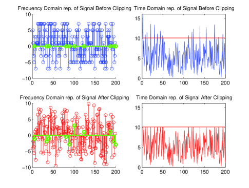
Fig. 1 illustrates the main points we’ve described so far, although caution must be taken as the actual OFDM signal is generally complex.

The block diagram in Fig. 2 stresses that upon observing $y$, the receiver is confronted with two estimation problems, the first is the typical estimation of the transmitted (clipped) OFDM signal $\bar{x}$, and the second is the estimation of the peak reducing signal $c$. Although the noise statistics are the same in both cases, the estimation SNR is nevertheless very different, depending on the clipping procedure. We will hence reserve the SNR notation for the received signal-to-noise-ratio and denote by CNR the clipper-to-noise-ratio which is defined as

CNR $$= \frac{E\left[\|\Psi c\|^{2}\right]}{E\left[\|\acute{z}\|^{2}\right]}$$ (7)

$$= \frac{E\left[\|\sum_{k\in\mathcal{I}_{c}}c(k)\psi_{k}\|^{2}\right]}{\sigma_{z}^{2}}$$

and hence depends on the sparsity level $\|c\|_{0}=|\mathcal{I}_{c}|$ and the magnitudes of $\{c(k)\}_{k\in\mathcal{I}_{c}}$ which are both functions of the clipping threshold $\gamma$. This is the parameter of concern when it comes to compressive sensing in this paper. By definition, the CNR is typically less than the SNR since the energy of $c$ leaks onto all the subcarriers even though the CS algorithm only has access to $\frac{m}{N}$ of them, and also since the magnitudes of the nonzero coefficients of $c$ are practically smaller than those of $x$.

Figure 2: Block Diagram of Basic Design

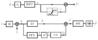
Note that in using CS our objective is to find the support $\mathcal{I}_{c}$ of the sparse signal and its complex coefficients $\{v(k)\}_{k\in\mathcal{I}_{c}}$ at those locations. We could hence decompose the two problems into $c=\textbf{S}_{c}v_{c}$ and use CS for the first problem only, giving us $\hat{\textbf{S}}^{(cs)}_{c}$ based on $\hat{\mathcal{I}}^{(cs)}_{c}$, then refine our coefficient estimate by a more robust technique such as lease squares after conditioning on the detected support. To do so we define the $m\times s$ matrix $\hat{\Phi}=\Psi\hat{S}^{(cs)}_{c}$ and refine our amplitude estimate to

$$\hat{v}^{(ls|cs)}_{c}=(\hat{\Phi}^{H}\hat{\Phi})^{-1}\hat{\Phi}^{H}\acute{y}$$ (8)

in which $\hat{c}^{(cs,ls)}=\hat{\textbf{S}}^{(cs)}_{c}\hat{v}^{(ls|cs)}_{c}$ follows. This dual approach is necessary in order to approach an oracle receiver that uses least squares (see the interesting discussion in [42]).

IV Comparison with Typical Tone-Reservation PAPR Reduction Techniques

The common function of reserved tones in the literature is to act as a frequency support for the peak reducing signal that is disjoint from the data-carrying tones [17, 19, 18, 23, 22, 24]. In other words, for each OFDM signal a search is conducted for some signal $c$ that will reduce the PAPR while being spectrally confined to a limited number of tones such that $\|\check{c}\|_{2}-\|\textbf{S}_{m}^{T}\check{c}\|_{2}=0$ and hence $\check{c}^{\,H}\check{d}=0$. Although many different methods exist to find such a signal, we only mention the well-known work of Tellado’s [17] for brevity, which requires solving the convex optimization problem

$$\min_{\check{c}}\quad t$$

$$s.t.\>\|x+\textbf{F}^{H}\textbf{S}\check{c}\|^{2}\leq t$$ (9)

where $\check{c}=\textbf{F}c$ is nonzero only on $\Omega_{c}$ from the definition of S. Clearly, this optimization approach should result in significantly more PAPR reduction compared to our design, since for the same number of reserved tones $m$, we can only clip $s<m$ maximum peaks, whereas by Tellado’s method no such restriction exists.

Most importantly however, the main complexity (i.e. the stage at which the optimization search is performed) in these techniques is at the transmitter, since the main concern is to find $c$ that will reduce the PAPR while occupying completely disjoint tones in order to remain discernable at the receiver.

V Enhanced PAPR Reduction by Data-Induced Weighted and Phase-Augmented $\ell_{1}$ Minimization

So far we were only interested in using compressive sensing in its most abstract form as it applies to our problem. We assumed, following the general literature on CS, that absolutely no information is known about the locations, magnitudes, and phases of the sparse signal $c$, beyond the incomplete frequency observations which we obtained from the reserved tones $\Omega_{c}$ [31, 32]. In other words, the model $\acute{y}=\Psi c+\acute{z}$ was assumed to exist independently of the general transceiver model $y=H\bar{x}+z$, even though in reality we know that $c$ is intimately linked to $\bar{x}$ by the simple fact that it’s superimposed on $x$ in the time domain.

The upshot of this section is to demonstrate that for optimal PAPR reduction using CS, the estimation of the clipping signal at the receiver should exploit as much information as possible in both basis representations, which can be achieved by weighting, constraining, or rotating the frequency-based CS search, based on information we infer from the data in the time domain.

The difficulty of these problems is strongly related to the way clipping is performed. Although we have full control in selecting the sparsity level and the clipping magnitudes and phases to best suite our purpose, there can’t be a clipping technique that optimizes both the support recovery and coefficient estimation, and a compromise must be made regarding the quality of the two.

V-A Homogeneous Clipping Techniques

we first begin with defining two simple clipping techniques that do not require any optimization or spectral confinement, and although we derive their PDFs along other properties, we focus exclusively on deterministic CS enhancement techniques, and delay the matter of Bayesian compressive estimation or sensing to the following section.

V-A1 Peak Suppression to $\gamma$ (PS)

Because clipping is done on the coefficients of $x$ whose envelope exceed $\gamma$, the most natural construction of the clipping signal $c$ would be to basically suppress the magnitudes of the entries $x_{i}:|x_{i}|\geq\gamma$ to $\gamma$ while preserving their angles, such that $|x_{i}+c_{i}|=\gamma$ (see Fig. 3). This is commonly expressed in the literature [58, 60] as

$$\bar{x}(i)=\begin{cases}\gamma e^{\;j\theta_{x(i)}}\;&\mbox{if}\;|x(i)|>\gamma,\\ \,\,\,\,x(i)\;&\mbox{otherwise}\end{cases}$$ (10)

Obviously, the PDF of the nonzero coefficients of $c^{ps}$ will depend on the PDF of $|x|\big{|}|x|>\gamma$. Hence if we define the binary set $\mathcal{Q}$ to label the mutually exclusive events of clipping or not at a certain index $i$ then

$$f(|c^{ps}|(i)) = \sum_{q\in\mathcal{Q}}P\left(|c^{ps}(i)|\,|q\right)P(q)$$ (11)

$$= f_{|X|||X|>\gamma}(|c^{ps}(i)|+\gamma)\left(\bar{\mathbbm{F}}_{|X|}(\gamma)\right)$$

$$\quad\quad+\;\delta(|c^{ps}(i)|)\mathbbm{F}_{|X|}(\gamma)$$

$$= \alpha^{-1}(\gamma)\left(\bar{\mathbbm{F}}_{|X|}(\gamma)\right)f_{|X|}(|c^{ps}(i)|+\gamma)$$

$$\quad\quad\cdot\;u(|c^{ps}(i)|)+\mathbbm{F}_{|X|}(\gamma)\delta(|c^{ps}(i)|)$$

where $u(\cdot)$ is the unit step function and $\alpha(\gamma)=\int_{\gamma}^{\infty}f_{|X|}\left(|x|\right)dx$ is a normalizing constant which depends only on $\gamma$ and is required to ensure that $\int_{0}^{\infty}f_{|X|||X|>\gamma}\left(|x|||x|>\gamma\right)d|x|=1$. Not surprisingly, this is the most popular soft clipping scheme due to its simplicity and relatively low spectral distortion.

Two features of this clipping scheme stand out in regard to CS enhancement. The first is that by suppressing all the data coefficients to a fixed and known threshold value $\gamma$, we could actually infer some additional information regarding possible clipping locations from the distance between the estimated coefficients’ magnitudes and $\gamma$. This clipping scheme can hence provide additional information regarding the support $\mathcal{I}_{c}$. The second feature is that the nonzero coefficients of $c^{ps}$ are exactly anti-phased with the data coefficients at $\mathcal{I}_{c}$, giving us another source of information regarding the phases $\theta_{c^{ps}(\mathcal{I}_{c})}$ based on $\hat{\bar{x}}$.

Figure 3: Peak Suppression Illustrated on the Complex Plane

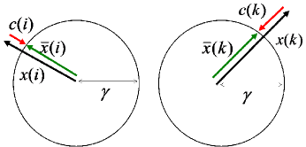
In terms of delectability from standard compressive sensing, however, the method is quite un-satisfying if left un-enhanced, demanding a higher number of measurements for the same sparsity level and Symbol Error Rate (SER) compared to other clipping techniques. The main reasons are

1. Low CNR: The CNR in PS decreases very rapidly with $\gamma$. Assuming we neglect the effect of $\Psi$,

   $$E[\|c^{ps}\|^{2}] = \sum_{k\in\mathcal{I}_{c}}E\left[|c^{ps}(k)|^{2}|\right]$$ (12)

   $$= E\left[|c^{ps}(k)|^{2}\right]\cdot E[\|c\|_{0}]$$

   $$= \int_{\infty}^{\infty}|c^{ps}(k)|^{2}f(|c^{ps}(k)|)d|c^{ps}(k)|$$

   $${}\quad\quad\cdot E[\|c\|_{0}]$$

   $$= \left[\alpha^{-1}(\gamma)(2\sigma_{|X|}^{2}+\gamma^{2})e^{-\frac{\gamma^{2}}{2\sigma_{|X|}^{2}}}-\gamma\right]$$

   $${}\quad\quad\cdot E[\|c\|_{0}]$$

   where the average sparsity

   $$E[\|c\|_{0}] = N^{2}\left(\bar{\mathbbm{F}}_{|X|}(\gamma)\right)^{2}-N\left(\bar{\mathbbm{F}}_{|X|}(\gamma)\right)^{2}$$

   $${}\quad\quad+N\left(\bar{\mathbbm{F}}_{|X|}(\gamma)\right)$$

   is simply the expectation of the Binomial corresponding to the sparsity level. Notice the accumulative effect of $\gamma$ on $E[\|c^{ps}\|^{2}]$.

2. The vanishing of $|c^{ps}_{min}|$: the random magnitudes of $c^{ps}$ are drawn from the tail distributions of the data coefficients, making the limiting distance between the minimum penetrating coefficient and $\gamma$ approach zero. This is a critical bottleneck in CS that cannot be completely compensated for by increasing the CNR. Fletcher et al. [41] and Wainwright [42, 43, 44] stress this point.

V-A2 Digital-Magnitude Clipping (DMC)

Figure 4: Clipping with Fixed Magnitude $\zeta$

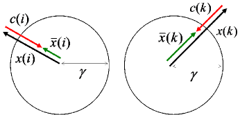
In order to avoid the problems of the previous clipping technique, we could increment the magnitudes of $c^{ps}$ by some constant until we’re satisfied with the CNR and $|c^{ps}_{min}|$. This however still leaves us with the burden of estimating the random magnitudes while destroying the enhanced support detection property of peak suppression. Instead, consider inverting the procedure from suppressing to a fixed value $\gamma$, to suppressing by a fixed value $\zeta$.

Now that $\{|c(k)|\}_{k\in\mathcal{I}_{c}}=\zeta$, we’ve decreased the degrees of freedom of $c$ to $\mathcal{I}_{c}$ and $\theta_{c}$ only. Furthermore, such a clipping scheme preserves the anti-phase property as well, thus possibly reducing the problem to that of support detection.

More generally, we could suppress the high peaks of $x$ by a finite set of magnitudes $\{\zeta_{0},\zeta_{1},\ldots,\zeta_{\ell}\}\in\mathbbm{Z}^{\ell}$, hence the attribute of Digital Magnitude Clipping (or simply Digital Clipping for short), although we will only focus here on the binary magnitude space $|c|\in\{0,\zeta\}$.

Following the same procedure in finding (11), and by noting the interesting relation $\|c\|_{p}=\zeta\|c\|_{0}^{{}^{1/p}},\,\,p=1,2,..,$ the PDF of the clipping signal’s envelope is basically

$$f\left(|c|^{dm}(i)\right)=\left(\bar{\mathbbm{F}}_{|X|}(\gamma)\right)\delta\left(|c|-\zeta\right)+\mathbbm{F}_{|X|}(\gamma)\delta\left(|c|\right).$$ (13)

The PDF of a coefficient’s magnitude has been reduced to a Bernoulli random variable with probability of success $\left(\bar{\mathbbm{F}}_{|X|}(\gamma)\right)$. Furthermore, the two clipping methods PS and DMC achieve the same CNR when

$$\zeta=\sqrt{\alpha^{-1}(\gamma)\left(2\sigma_{|X|}^{2}+\gamma^{2}\right)e^{\gamma^{2}/2\sigma_{|X|}^{2}}-\gamma}.$$ (14)

There is a conflicting interest in deciding the value of $\zeta$. On one hand, the more we increase it the higher the CNR and the easier the support detection becomes, but on the other, the overall error of the system dramatically increases in case of faulty support detection. Furthermore, oversampling at the subsequent stage of transmission becomes more complex in this latter case.

Nevertheless, we should at least set a lower bound on its value to ensure that all clipped coefficients will always end up with magnitudes equivalent to or bellow the desired clipping threshold $\gamma$, depending on the envelopes maximum order statistic. Afterwards, we should be very conservative in increasing $\zeta$

V-B Externally Weighted $\ell_{1}$ Minimization

If by some prior information we have a better picture regarding the support $\mathcal{I}_{c}$ beyond the Bernoulli process assumption, we can modify the LASSO in (6) by penalizing disfavored locations so that

$$\hat{c}=\arg\min\|\acute{y}-\Psi c\|_{2}^{2}+\lambda\|w^{T}c\|_{1},$$ (15)

where $w$ is a weighting vector imposed on the $\ell_{1}$ penalty term based on this prior information. In the literature, the source of $w$ is from previous runs of the CS algorithm itself [34][55], where the hope is that with each iteration more confidence will exist in $\hat{\mathcal{I}}^{(k+1)}_{c}$ based on, for instance [34],

$$w(i)^{(k+1)}\propto\left[\;|\hat{c}(i)^{(k)^{cs}}|+\epsilon\right]^{-1}\qquad i=1,2,\ldots,N$$ (16)

where $\epsilon>0$ is a small stabilizing parameter. We will refer to this procedure as internally weighted $\ell_{1}$ minimization.

Repeating the CS algorithm is computationally expensive, and the process is sensitive to the quality of the first unguided CS estimate. Instead, we would rather use a one-shot weighting scheme that minimally increases the complexity of an ordinary LASSO. Fortunately, this could be done if we had an external source of information based on the data vector $\hat{\bar{x}}$.

Recall the discussion in V-A1 regarding embedded information on the support $\mathcal{I}_{c}$ in peak suppression. The idea is that we expect the coefficients of $\hat{\bar{x}}$ whose magnitudes are close to $\gamma$ to be more probable clipping locations compared to ones that are not. Consequently, we can define a weighting vector $w^{ps}$ based on the distance

$$d(i)=||\hat{\bar{x}}(i)|-\gamma|,\qquad i=1,2,\ldots,N$$ (17)

and use it in (15). Another data-based weighting scheme would be the posterior probability of not having a clip ($q=0$) given the observation (17), such that less likely clipping locations are more severely penalized by having a higher such posterior probability

$$w(i)^{ps} = \Pr\left(q=0\,|\,d(i)\right)$$

$$= \frac{\Pr(d(i)|q=0)\Pr(q=0)}{\sum_{q\in\mathcal{Q}}\Pr(d(i)|q)\Pr(q)}$$

$$= \frac{f_{|\hat{X}|}(\gamma-d(i))\mathbbm{F}_{|X|}(\gamma)}{f_{|\hat{X}|}(\gamma-d(i))\mathbbm{F}_{|X|}(\gamma)+f_{|E|}(d(i))\bar{\mathbbm{F}}_{|X|}(\gamma)}$$

where $f_{|E|}$ is the density function corresponding to the estimation error of the data envelope $|\hat{x}|(i)$, which is the sole reason $d(i)\!>\!0$ when conditioned on clipping $x(i)$. Using least squares to recover $x(i)$, we assume its error to be Gaussian and hence $f_{|E|}$ and $f_{|\hat{X}|}=f_{|X+E|}$ to be Rayleigh with parameters $\sigma_{|E|}$ and $\sigma_{|X+E|}=\left[2^{-1}(\sigma_{X}^{2}+\sigma_{E}^{2})\right]^{1/2}$, respectively. Defining $\eta(\gamma)=1-e^{-\gamma^{2}/\sigma_{X}^{2}}$, this becomes

$$w(i)^{ps} = \frac{\diamondsuit e^{\clubsuit}}{\diamondsuit e^{\clubsuit}+\triangle e^{\spadesuit}}$$

$$= \begin{cases}\frac{\diamondsuit}{\diamondsuit+\triangle e^{\spadesuit-\clubsuit}};&\mbox{if}\;|\clubsuit|>|\spadesuit|,\\ \frac{\diamondsuit e^{\clubsuit-\spadesuit}}{\diamondsuit e^{\clubsuit-\spadesuit}+\triangle}&\mbox{if}\;|\spadesuit|>|\clubsuit|\end{cases}$$

where

$$\diamondsuit=\frac{2\eta(\gamma)(\gamma-d(i))}{\sigma_{X}^{2}+\sigma_{E}^{2}} \clubsuit=\frac{(\gamma-d(i))^{2}}{\sigma_{X}^{2}+\sigma_{E}^{2}}$$ ,

$$\triangle=\frac{2(1-\eta(\gamma))d(i)}{\sigma_{E}^{2}} \spadesuit=\frac{d(i)^{2}}{\sigma_{E}^{2}}.$$ ,

The second part of (V-B) is a necessary manipulation for numerical stability.

Notice also that what helps in suppressing only to $\gamma$ here is that we have a probabilistic means to cast out most of the possible false positives. Had we suppressed the magnitudes to the envelope mean for instance, $E[|x(i)|]$, the procedure above would favor many locations as clipping positions by the fact that $|\hat{\bar{x}}|-E[|x(i)|]$ is small. Nonetheless, misleading bias to certain locations as candidates for clipping positions due to their coefficient’s natural proximity to $\gamma$ can never be completely eliminated, even at infinite CNR.

V-C Phase-Augmented CS for Homogenous Clippers

In the case of homogenous clipping, $\theta_{c}(\mathcal{I}_{c})=\theta_{\bar{x}}(\mathcal{I}_{c})$ at the transmitter, and consequently the CS algorithm should have access to additional information regarding the phases of the nonzero coefficients. The problem however is that we only have an estimate $\theta_{\hat{\bar{x}}}(\mathcal{I}_{c})$ at the receiver, and the extent to which CS can benefit from this property depends on how good the estimate $\hat{\bar{x}}$ is in general. To this end, we will only consider the SNR as the parameter to which we judge the quality of the data estimate.

Recall the discussion following Fig. 2 regarding the CNR and SNR, and consider the effect of gradually increasing $\zeta$ which we defined in V-A2. Notice that when $\zeta=0$, the $\gamma$-penetrating coefficient attains its maximum SNR, then as we increase $\zeta$ the CNR increases as $\zeta^{2}E\left[\|c\|_{0}\right]$ while the SNR decreases by $\zeta\left(2E[|x|]-\zeta\right)$. Consequently, the CNR will be larger than the SNR in the locations where $\left(E\left[\|c\|_{0}\right]-1\right)\zeta^{2}+2E\left[|x|\right]\zeta-E\left[|x|^{2}\right]>0$. Fortunately practical values of $\zeta$ relative to $E\left[|x|\right]$ fall outside this region, and we would normally expect to gain information regarding $\theta_{c}$ from $\hat{\bar{x}}$ that is more reliable than information from CS alone.

This fact encourages us to absorb, and perhaps even replace altogether, as much information as possible regarding $\theta_{c}$ from the estimated data vector $\hat{\bar{x}}$. Assume first that we know the vector $\theta_{c}$, we could then merge this information into the CS algorithm by expressing the clipping signal as $c=\Theta_{c}|c|$ such that

$$c=\begin{bmatrix}e^{\,j\theta_{c(1)}}&0&0&0\\ 0&e^{\,j\theta_{c(2)}}&0&0\\ 0&0&\ddots&0\\ 0&0&0&e^{\,j\theta_{c(N)}}\end{bmatrix}\cdot\begin{bmatrix}|c(1)|\\ |c(2)|\\ \vdots\\ |c(N)|\end{bmatrix},$$

which could be directly fused into the measurement matrix $\Psi$, thus transforming our model from $\acute{y}=\Psi c+\acute{z}$ to $\acute{y}=\Psi\Theta_{c}|c|+\acute{z}$ where

$$\Psi\Theta_{c}=\begin{bmatrix}|&|&&|\\ e^{\,j\theta_{c(1)}}\psi_{1}&e^{\,j\theta_{c(2)}}\psi_{2}&\dots&e^{\,j\theta_{c(N)}}\psi_{N}\\ |&|&&|\end{bmatrix}$$

has now realigned the phases of the coefficients sought and reduced the problem to estimating a real sparse vector, with only the locations and magnitudes of the nonzero coefficients of $c$ to be found. In the case of digital clipping, we can then force the magnitudes to the nearest alphabets as well. In any case, with $\Theta_{c}$ unknown prior to CS, we will instead use $\Theta_{\hat{\bar{x}}}-2\pi\textbf{I}_{N\times N}$ to augment the CS algorithm. This could be done in two ways:

1. Sense then Rotate (StR): Use the standard CS or weighted CS algorithms used so far to regain $\hat{c}^{\,\textmd{NoPA}}=\arg_{c\,\in\textbf{C}^{N}}\min\{\|\acute{y}-\Psi c\|_{2}^{2}+\lambda\|c\|_{1}\}$ where PA stands for Phase Augmentation, extract the locations and magnitudes of the nonzero coefficients from $\hat{c}$, and then rotate them according to the corresponding estimated directions in $\hat{\bar{x}}$. i.e.

   $$\left\{\hat{c}^{\,\textmd{StR}}(i)\right\}_{i\in\hat{\mathcal{I}}_{c}}=\left\{|\,\hat{c}^{\,\textmd{NoPA}}(i)|\,e^{j\left(\theta_{\hat{\bar{x}}(i)}-2\pi\right)}\right\}_{i\in\hat{\mathcal{I}}_{c}}$$ (21)

2. Rotate then Sense (RtS): In this case supply the CS algorithm with the phase information from $\hat{\bar{x}}$ as described above. This rotation prior to compressive sensing recasts the problem as an estimation of a real vector with $2m$ real observations. Defining $\tilde{\Psi}_{c}=\Psi\Theta_{c}$, we’re left with the following model

   $$\tilde{y}=\left[\begin{array}[]{c}\Re\acute{y}\\ \Im\acute{y}\end{array}\right]=\left[\begin{array}[]{c}\Re\tilde{\Psi}_{c}\\ \Im\tilde{\Psi}_{c}\end{array}\right]\cdot|c|+\left[\begin{array}[]{c}\Re\acute{z}\\ \Im\acute{z}\end{array}\right]$$ (28)

   for which we use the following program to recover $c$

   $$\hat{c}^{\,\textmd{RtS}}=\arg_{|\,c\,|\in\,\textbf{R}^{N}}\min\left\{\|\tilde{y}-\tilde{\Psi}_{\hat{\bar{x}}}\,|\,c\,|\,\|_{2}^{2}+\lambda\|c\|_{1}\right\}$$ (29)

   where $\tilde{\Psi}_{\hat{\bar{x}}}=\Psi\left(\Theta_{\hat{\bar{x}}}-2\pi\textbf{I}_{N\times N}\right)$. Notice that, similar to (21) one could also replace the phases of $\hat{c}^{\,\textmd{RtS}}$ with $\left\{e^{j\left(\theta_{\hat{\bar{x}}(i)}-2\pi\right)}\right\}_{i\in\hat{\mathcal{I}}_{c}}$ after (29) but we have not observed any significant improvement in doing so.

VI Bayesian Estimation of Sparse Clipping Signals

To take into account the statistical information at hand, we could simply modify the dual stage estimate in (8) to a linear minimum mean-square (LMMSE) estimate of the amplitudes $v_{c}$ conditioned on the support estimate $\hat{\mathcal{I}}^{cs}_{c}$

$$\hat{v}_{c}^{lmmse|\hat{\mathcal{I}}^{cs}_{c}}=\sigma_{v_{c}}^{2}\hat{\Phi}^{H}\left(\sigma_{v_{c}}^{2}\hat{\Phi}\hat{\Phi}^{H}+\sigma_{z}^{2}I\right)^{-1}\left(\acute{y}-\hat{\Phi}E_{v_{c}}\right).$$

This should clearly improve upon the least square estimate (8) in case the distribution of $v_{c}$ is Gaussian, but will not be able to invoke any statistical information into the support estimate. Using a Maximum a Posteriori (MAP) estimate $\hat{c}=\arg\max P(\acute{y}|c)P(c)$ generally leads to non-convex optimization problems in sparse models, and we refer instead to an MMSE estimate. First define $J^{|\mathcal{I}|}$ as the Hamming vector of length $N$ and Hamming weight $|\mathcal{I}|$ with active coefficients according to the support set $\mathcal{I}$. Then marginalizing on all such possible vectors we obtain

$$\hat{c}^{\,\textmd{MMSE}} = E\left[\,c\,|\,\acute{y}\,\right]$$ (30)

$$= \sum_{i=1}^{2^{N}}E\left[\,c\,|\;\acute{y},J_{i}\right]P(\acute{y}|J_{i})P(J_{i})$$

with dropping off $P(\acute{y})$ in (30) due to its independence of $i$. The estimate is a weighted sum of conditional expectations, and the formal (exact) approach requires computing $2^{N}$ terms which is a formidable task for large $N$. To limit the search space, the key is to truncate the summation index to a much smaller subset of support vectors $\textbf{J}^{*}$. As such, the weights $\{P(J_{k}|\acute{y})\}_{k\in J^{*}}$ will not sum up to unity, and we will need to mitigate this by normalizing the truncated weighted sum by the sum of weights $\mathcal{W}=\sum_{k\in\textbf{J}^{*}}P(\acute{y}|J_{k})P(J_{k})$, hence reducing (30) to

$$\hat{c}^{\,\textmd{MMSE}} \approx \frac{1}{\mathcal{W}}\sum_{k\in\textbf{J}^{*}}E\left[\,c\,|\;\acute{y},J_{k}\right]P(\acute{y}|J_{k})P(J_{k}).$$ (31)

In effect, estimating $c$ in an MMSE criterion boils down to appropriately selecting $\textbf{J}^{*}$ and evaluating the terms $P(J_{k})$, $P(\acute{y}|J_{k})$, and $E\left[\,c\,|\;\acute{y},J_{k}\right],\forall J_{k}\in\textbf{J}^{*}$, which are in increasing complexity in the order we’ve just mentioned.

When using peak suppression to $\gamma$, the receiver is given a vague picture of where clipping has occurred based on the affinity of $\hat{\bar{x}}$ to $\gamma$. Consequently, by sorting the magnitudes of the weighting vector $w^{\downarrow}$ in (17) in ascending order, the probability of the true support coinciding with the first $\beta$ elements in $\arg\{w^{\downarrow}\}$ will increase rapidly with $\beta$. Fig. 5 shows a Monte Carlo simulation of this probability at different clipping thresholds. For instance, this implies that given a clipping threshold of $\gamma=2\sigma_{|X|}$, one could exclude $70\%$ of the $N$ indices as having too low a probability of corresponding to a clipping location, thus reducing the possible candidates from $2^{N}$ to $2^{\beta}$ Hamming vectors.

Figure 5: Probability of support index set $\mathcal{I}_{c}$ being completely included in the first $\beta/N\%$ of $\arg\{w^{\downarrow}\}$

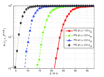
Given this reduced set $\textbf{J}^{\{k:k\leq\beta\}}$ of vectors, we adopt a search over it by latching a vector of unity Hamming weight based on (31), and then proceed in a greedy fashion similar to Larsson [49] and Schniter [50, 51] until a maximum sparsity level $s^{max}$ is reached. This will preserve the quality of the greedy estimate using Fast Bayesian Matching Pursuit (FBMP) in [50] while reducing the number of executions of (31) by

$$100\left(1-\frac{\beta(1+\rho\cdot s^{max})-\frac{\rho\cdot s^{max}(s^{max}+1)}{2}}{N(1+\rho\cdot s^{max})-\frac{\rho\cdot s^{max}(s^{max}+1)}{2}}\right)\%$$

where $\rho$ is the number of tested candidates for each Hamming weight. This would correspond to a reduction of $60-80\%$ of executions with our practical parameters, and we will henceforth refer to this procedure as $\beta$-FBMP.

VII Performance Analysis and Simulations

For our simulation purposes we considered an OFDM signal of $N=256$ subcarriers of which $m=0.2N$ are randomly dispersed measurement tones. The data coefficients were generated from a QAM constellation of size $M=32$. The Rayleigh fading channel model was of 32 taps, operating at a $30$ dB SNR environment. The performance parameters we considered were the SER, the relative temporal complexity, the PAPR reduction ability, and the capacity.

Our primary objective was to test the SER variation with the clipping threshold $\gamma$ for a clipped OFDM signal that used our different adaptations of CS algorithms and clipping techniques. Observed as a variable, the clipping threshold in particular is of central importance due to its critical effect on both CS generic performance and the PAPR reduction. Decreasing $\gamma$ significantly reduces the PAPR but also implies a nonlinear increase in the average sparsity level that the estimation algorithms must tolerate. It also has a positive counter effect on CS performance as well since it increases the CNR, making the overall behavior of SER($\gamma$) difficult to predict.

Furthermore, when testing the precise performance of an algorithm we used the Normalized Mean Square Error

NMSE $$= E\left[\frac{(c-\hat{c})^{2}}{\|c\|_{2}^{2}}\right]$$

to ensure that error decrease was not simply due to a decrease in the number of estimated variables.

Figure 6: SER of PS vs $\gamma$

Figure 7: NMSE of Digital Clipper estimate as a function of the coefficient magnitude $\zeta$

Figure 8: NMSE of Digital Clipper Estimate as a function of the clipping threshold $\gamma$

Figure 9: SER of Digital Clipping with $\zeta=0.8\,\sigma_{|X|}$ vs $\gamma$

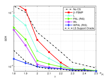
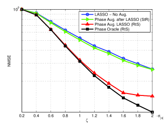
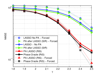
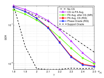
Fig. 6 shows the SER for Peak Suppressing clippers in V-A1 after QAM decoding $(\textbf{F}\textbf{S}_{x})^{\dagger}(\hat{\bar{x}}^{ls}+\hat{c}^{(ps)})$ as the clipping threshold is varied. The methods tested were the reduced search space greedy method ($\beta$-FBMP), the LASSO, the Phase-Augmented LASSO (PAL) using (29), the data-based Weighted LASSO (WL), and the Weighted Phase-Augmented LASSO (WPAL). These were compared against two performance bounds: the lower bound of not estimating $c$, and the upper bound of an oracle receiver that knows the support $\mathcal{I}_{c}$, and simply uses least squares to estimate the coefficients’ amplitudes. Interestingly, combining the support and phase augmentation techniques into the LASSO enables it to perform very close to the support oracle, and even beat it at low clipping thresholds where $s>0.55\,m$ since it has additional information regarding the coefficients’ phases. Furthermore, weighting alone is more effective then phase-augmentation, although both significantly improve the performance of the LASSO.

To see the effect of varying the magnitude of active coefficients in digital clipping of section V-A2 we plotted the NMSE vs $\zeta$ in Fig. 7. This avoids a biased evaluation due to increased CNR with $\zeta$. The results imply that embedding the phase information into the LASSO in (29) is much more effective than rotating the estimate after compressed sensing in (21). It also shows that the former method is considerably close to a phase oracle that uses the same technique for practical values of $\zeta$ relative to $\sigma_{|X|}$. However, as expected they eventually deviate as we increase $\zeta$ since this corresponds to decreasing the SNR and hence the accuracy of the phase information induced from the data vector estimate $\theta_{\hat{\bar{x}}}$. Fig. 8 implies that forcing the magnitudes of the estimates in (21) and (29) is generally ineffective except in the very sparse cases for the former. The overall result on the SER is portrayed in Fig. 9 at a fixed $\zeta=0.8\,\sigma_{|X|}$.

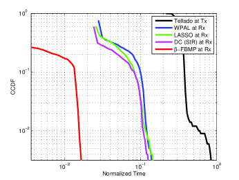
Complexity-wise, we neglect mentioning implementation and orders of complexity since they match those of standard algorithms we’ve built on and that are well documented in the CS literature (e.g. [39, 50, 53]). Instead we investigate the practical aspect of the relative time required to execute the major techniques proposed in the paper compared to Tellado’s primary tone-reservation algorithm using the same generic CVX software [52]. As such we collected the random execution times for $2000$ runs of each, normalized them by the maximum execution time among all, and plotted their CCDF. Fig. 10 depicts the results. Roughly speaking, the methods stemming from the LASSO required less then $12\%$ of the time required to execute Tellado’s primary QCQP algorithm on average, while the $\beta$-FBMP required less than $2\%$ of the time.

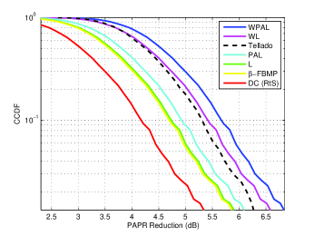
A major advantage of clipping to a fixed threshold is that, unlike tone-reservation methods such as [17, 22] the dynamic range, maximum power, and PAPR of the transmitted signal are fixed. The distribution of PAPR reduction, $10\log_{10}\left(\frac{P_{max}}{\gamma^{2}}\right)$, would simply follow from the distribution of the maximum squared coefficient in $x$ (refer to [57, 58, 59] for relevant analysis) which we plot in Fig. 11. The fixed maximum power followed from the clipping threshold that corresponded to a SER of $10^{-2}$ for the different techniques in this work.

TABLE I: Summary of Results

	Tolerable $\gamma$	Avg. PAPR Red. (dB)	$\%$ Exec. Time
DC (RtS)	2.40 $\cdot\,\sigma_{|X|}$	3.19	$11.06\%$
$\beta$-FBMP	2.26 $\cdot\,\sigma_{|X|}$	3.71	$1.6\%$
LASSO	2.25 $\cdot\,\sigma_{|X|}$	3.75	$12.3\%$
WPAL	2.02 $\cdot\,\sigma_{|X|}$	4.68	$13.9\%$
Tellado	-	4.37	$100\%$

The most fundamental parameter of interest given a desired clipping threshold is the channel capacity [17, 60]

$$C=\sum_{k=1}^{N}\log_{2}\left(1+\frac{|D(k,k)|^{2}\sigma_{x(k)}^{2}}{\sigma_{z(k)}^{2}}\right),$$

and we will thus consider two systems. The first system $\mathcal{S}_{1}$ clips all coefficients above $\gamma$ and does not reserve tones to estimate the clipping signal $c$, resulting in a higher clipping noise over all $N$ tones while retaining all of them for data transmission. The second system $\mathcal{S}_{2}$ reserves $m$ tones to estimate $c$, thus reducing the SER degradation while also reducing the data tones by $m$.

Figure 10: CCDF of execution time normalized by maximum value

Figure 11: CCDF of PAPR Reduction (dB)

The justification then depends very much on the variances of the clipping noise $\{\sigma_{c}^{2}(k;\gamma)\}_{k\in\Omega_{d}}$ with and without estimation at the receiver. Furthermore, if the threshold $\gamma$ is sufficiently low relative to $\sigma_{|X|}$ (e.g. $E\left[\|c\|_{0}\,;\gamma\right]=10\%$ of $N$), the clipping noise on each tone will be the result of a reasonably large summation of scaled coefficients of $c$ in the time domain, and so will the distribution of the priors in (11) converge to a Gaussian. With this theoretical justification aided by extensive simulations, we will assume for simplicity that the distortion on each carrier follows a Gaussian with a common variance $\sigma_{c}^{2}$. However, caution must be taken when comparing this parameter for the two systems. The reason is that $\mathcal{S}_{1}$ has more data energy than $\mathcal{S}_{2}$ by using all $N$ tones, and will thus have a higher distortion variance at the same clipping level $\gamma$, i.e. $\sigma_{c\,\mid|\Omega_{d}|=N}^{2}>\sigma_{c\,\mid|\Omega_{d}|=N-m}^{2}$. Consequently, the capacity of the first system (after dropping the tone index) will be

$$C_{1}=N\log_{2}\left(1+\frac{|D|^{2}\sigma_{x\,\mid|\Omega_{d}|=N}^{2}}{|D|^{2}\sigma_{c\,\mid|\Omega_{d}|=N}^{2}+\sigma_{z}^{2}}\right)$$ (32)

while the capacity of the second will be

$$C_{2}=(N-m)\log_{2}\left(1+\frac{|D|^{2}\sigma_{x\,\mid|\Omega_{d}|=N-m}^{2}}{|D|^{2}\sigma_{\left(c-\hat{c}\right)\mid|\Omega_{d}|=N-m}^{2}+\sigma_{z}^{2}}\right)$$ (33)

The use of reserved tones for CS is then justified if $C_{2}>C_{1}$, i.e. when

$$\sigma_{\left(c-\hat{c}\right)\mid|\Omega_{d}|=N-m}^{2}<\frac{\sigma_{x\,\mid|\Omega_{d}|=N-m}^{2}}{\left[1+\frac{|D|^{2}\sigma_{x\,\mid|\Omega_{d}|=N}^{2}}{|D|^{2}\sigma_{c\,\mid|\Omega_{d}|=N}^{2}+\sigma_{z}^{2}}\right]^{\frac{N}{N-m}}-1}-\frac{\sigma_{z}^{2}}{|D|^{2}}$$ (34)

Figure 12: Capacity per transmitted tone at different clipping thresholds

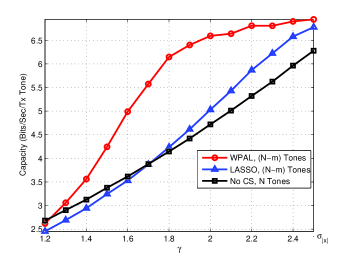
It would be very interesting to observe how this parameter behaves as a function of the clipping threshold $\gamma$ as both the distortion $\sigma_{c}^{2}$ and the quality of the estimate $\hat{\sigma}_{c}^{2}$ nonlinearly counteract each other. Fig. 12 shows such results upon $1000$ runs at each $\gamma$ for estimating $\sigma_{c}^{2}$ and $\sigma_{\left(c-\hat{c}\right)}^{2}$. The results show that by reserving $20\%$ of the tones for data-based weighted and phase-augmented LASSO the capacity of such a system can significantly outperform the naive system which uses all the tones for data transmission. What’s more, the capacity associated with this technique behaves in a convex fashion so that by reducing the capacity by less then 1 bit per second per transmitted tone, the clipping threshold can be dramatically reduced from $\gamma=2.5\,\sigma_{|X|}$ to $\gamma=2\,\sigma_{|X|}$. Unlike the semi-linear relation of $\mathcal{S}_{1}$ with $\gamma$, such behavior offers a very tempting compromise between capacity and peak-reduction. Using the typical LASSO at such conditions is effective at clipping thresholds reaching as low as $1.9\,\sigma_{|X|}$ which is impressive.

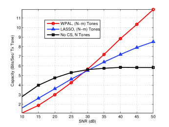
Fig. 13 implies that increasing the SNR is much more rewarding for $\mathcal{S}_{2}$ compared to $\mathcal{S}_{1}$ which we test at a fixed clipping threshold of $2.3\,\sigma_{|X|}$. The reason is that eliminating $\sigma_{z}^{2}$ has no effect on $\sigma_{c}^{2}$ and the capacity of the naive system saturates after an SNR of 35 dB. On the other hand, decreasing the noise level improves the CS estimate and hence has a dual effect in increasing the capacity, leading to the semi-linear relation with the SNR.

Figure 13: Capacity per transmitted tone vs SNR

VIII Conclusion

In this work we have established the new general concept of clipping mitigation (and hence PAPR reduction) in OFDM using compressive sensing techniques. The general framework stressed the use of reserved subcarriers to compressively estimate the locations and amplitudes of the clipped portions of a transmitted OFDM signal at the receiver, instead of using them at the transmitter as a spectral support for optimized peak reducing signals in the time domain. Consequently, the method interchanges the stage at which signal processing complexity is required compared to the previous techniques, hence introducing a real solution to communication systems that use OFDM signals at the physical layer and require minimal complexity at the transmitter.

The other major contribution is demonstrating how by a marginal increase in complexity one can augment the standard $\ell_{1}$ minimization of CS by extracting information regarding clipping locations, magnitudes, and phases from the data, and hence enable the system to estimate sparse clippers far beyond the recoverability conditions of CS (e.g. sparsity levels above $55\%$ of $m$). Such augmentation was shown to significantly boost the overall system’s capacity at low clipping thresholds and thus suggests a very appealing compromise between capacity and peak-reduction.

References

- [1] J. G. Andrews, A. Ghosh, R. Muhamed, Fundamentals of WiMAX: Understanding Broadband Wireless Networking, Prentice Hall, part of the Prentice Hall Communications Engineering and Emerging Technologies Series, 2007.
- [2] T. Jiang, W. Xiang, H. H. Chen, and Q. Ni, “Multicast broadcasting services support in OFDMA-based WiMAX systems,” IEEE Commun. Mag., vol. 45, no. 8, pp. 78 86, Aug. 2007.
- [3] S. Litsyn, Peak Power Control in Multicarrier Communications, Cambridge University Press, edition, Jan. 2007.
- [4] T. Jiang and Y. Wu, “An Overview: Peak-to-Average Power Ratio Reduction Techniques for OFDM Signals,” IEEE Trans. Broadcast., vol. 54, no. 2, June 2008.
- [5] S. H. Han and J. H. Lee, “An overview of peak-to-average power ratio reduction techniques for multicarrier transmission,” IEEE Pers. Commun., vol. 12, no. 2, pp. 56 65, Apr. 2005.
- [6] K. Sathananthan, C. Tellambura, “Coding to reduce both PAR and PICR of an OFDM signal,” IEEE Commun. Lett., vol.6, no.8, pp. 316-318, Aug 2002.
- [7] J. A. Davis and J. Jedwab, “Peak-to-Mean Power Control in OFDM, Golay Complementary Sequences, and Reed-Muller Codes,” IEEE Trans. on Inf. Theory, vol.45, No.7, Nov. 1999.
- [8] T. Jiang and G. X. Zhu, “Complement Block Coding For Reduction in Peak-To-Average Power Ratio of OFDM Signals,” IEEE Commun. Mag., vol. 43, no. 9, pp. 17 22, Sept. 2005.
- [9] R. W. Bauml, R. F. H. Fischer, and J. B. Huber, “Reducing the Peak-To-Average Power Ratio of Multicarrier Modulation by Selected Mapping,” Electronics Letters, vol. 32, no. 22, pp. 2056-2057, 1996.
- [10] A. Ghassemi and T. A. Gulliver, “A Low Complexity Selective Mapping OFDM using Multiple IFFT Stages,” International Journal of Communication Networks and Distributed Systems, vol. 1, Issue 2, Sep. 2008.
- [11] S. H. Muller and J. B. Huber, “OFDM with Reduced Peak-to-Average Power Ratio by Optimum Combination of Partial Transmit Sequences, Electronic Letters, vol. 33, no. 5, pp. 2056 2057, Feb. 1997.
- [12] A. Alavi, C. Tellambura, and I. Fair, “PAPR Reduction Of OFDM Signals using Partial Transmit Sequence: An Optimal Approach using Sphere Decoding,” IEEE Commun. Lett., vol. 9, no. 11, pp. 982 984, Nov. 2005.
- [13] Y. J. Kou, W. S. Lu, and A. Antoniou, “A New Peak-To-Average Power-Ratio Reduction Algorithm For OFDM Systems via Constellation Extension,” IEEE Trans. Wireless Commun., vol. 6, no. 5, pp. 1823 1832, May 2007.
- [14] M. Malkin, B. Krongold, and J. M. Cioffi, “Optimal Constellation Distortion For PAR Reduction In OFDM Systems,” PIMRC 2008, IEEE 19th International Symposium on Personal, Indoor and Mobile Radio Communications, 2008.
- [15] B. Crongold and D. Jones, “PAR Reduction in OFDM via Active Constellation Extension”, IEEE Trans. Broadcast., vol.49, iss.3, September 2003.
- [16] J. Tellado and J. M. Cioffi, “Peak Power Reduction for Multicarrier Transmission”, IEEE Globecom 99, Rio de Janeiro, Brazil, Dec. 5-9, 1999.
- [17] J. Tellado, Multicarrier Modulation with Low PAR Applications to DSL and Wireless, Kluwer Academic Publishers, Norwell 2000.
- [18] N. Andgart et al., “Designing Tone Reservation PAR Reduction,” EURASIP J. Appl. Signal Process., vol. 2006, pp 82-82, 2006.
- [19] B.S. Krongold and D.L. Jones, “An Active-Set Approach for OFDM PAR Reduction via Tone Reservation,” IEEE Trans. Signal Process., vol.52, no.2, pp. 495-509, Feb. 2004.
- [20] E. B. Al-Safadi and T. Y. Al-Naffouri, “On Reducing the Complexity of Tone Reservation Based PAPR Reduction Schemes by Compressive Sensing,” IEEE Globecom ’09, Honolulu HI, Nov. 2009.
- [21] J. C. Chen and C. P. Li, “ Tone Reservation Using Near-Optimal Peak Reduction Tone Set Selection Algorithm for PAPR Reduction in OFDM Systems,” IEEE Signal Process. Lett. vol. 17 no. 11 pp. 933-936, Nov. 2010.
- [22] J. Ilic and T. Strohmer, “PAPR Reduction in OFDM using Kashin’s Representation,” IEEE 10th Workshop on Signal Process. Advances in Wireless Commun., pp.444-448, Perugia, Italy, June 2009.
- [23] Fei Shao et al., “SOCP Approach for PAPR Reduction Using Tone Reservation for the Future DVB-T/H Standards,” Multi-Carrier Systems & amp Solutions, Springer Netherlands, 2009.
- [24] S. Janaaththanan, “A Gradient Based Algorithm for PAPR Reduction of OFDM using Tone Reservation Technique,” IEEE Veh. Tech. Conf., pp. 2977-2980, Singapore, May 2008.
- [25] T. Jiang, W. D. Xiang, P. C. Richardson, D. M. Qu, and G. X. Zhu, “On the Nonlinear Companding Transform for Reduction in PAPR of MCM signals,” IEEE Trans. Wireless Commun., vol. 6, no. 6, pp. 2017 2021, Jun. 2007.
- [26] T. Jiang, W. Yao, P. Guo, Y. Song, and D. Qu, “Two novel nonlinear companding schemes with iterative receiver to reduce PAPR in multicarrier modulation systems,” IEEE Trans. Inf. Theory, vol. 52, no. 2, pp. 268 273, Mar. 2006.
- [27] Tao Jiang, Yang Yang and Yong-Hua Song, “Exponential Companding technique for PAPR reduction in OFDM Systems”, IEEE Trans. Inf. Theory, vol. 51, no. 2, pp. 244 - 248, June 2005.
- [28] P. Xia, S. Zhou, and G.B Giannakis, “Achieving the Welch Bound with Difference Sets,” IEEE Int. Conf. on Acoustics, Speech, and Signal Processing, March 2005.
- [29] M. Stojnic et al., “On the Reconstruction of Block-Sparse Signals with an Optimal Number of Measurements,” IEEE Trans. on Signal Process., vol. 57 no. 8 pp. 3075-3085, 2009.
- [30] Y. C. Eldar and H. Bölcskei, “Block-Sparsity: Coherence and Efficient Recovery,” in Proc. IEEE International Conference on Acoustics, Speech and Signal Processing, pp.2885-2888, 2009.
- [31] E. J. Candes, J. Romberg and T. Tao. “Robust Uncertainty Principles: Exact Signal Reconstruction From Highly Incomplete Frequency Information,” IEEE Trans. Inf. Theory, vol. 52 pp. 489-509, 2004.
- [32] E. J. Candes, T. Tao. “Near-optimal signal recovery from random projections:universal encoding strategies?,” IEEE Trans. Inf. Theory, vol. 52 pp. 5406-5425, Dec. 2006.
- [33] E. J. Candes, J. Romberg and T. Tao. “Stable signal recovery from incomplete and inaccurate measurements,” Comm. Pure Appl. Math., vol. 59 pp. 1207-1223, 2005.
- [34] E. J. Candes, M. Wakin, and S. Boyd, “Enhancing sparsity by reweighted minimization,” J. Fourier Anal. Appl., vol. 14, no. 5, pp. 877.905, 2008.
- [35] E. J. Candes and Yaniv Plan, “Near-Ideal Model Selection by Minimization,” Preprint, 2007.
- [36] S. S. Chen, D. L. Donoho, and M. A. Saunders, “Atomic Decomposition by Basis Pursuit,” SIAM J. Sci. Comput. vol. 20, Issue 1, pp. 33-61 (1998).
- [37] D. Donoho, “Compressed Sensing,” IEEE Trans. Inf. Theory, vol. 52(4), pp. 1289 - 1306, April 2006.
- [38] J. A. Tropp, A. C. Gilbert “Signal Recovery from Random Measurements via Orthogonal Matching Pursuit,” IEEE Trans. Inf. Theory, vol. 53, no. 12, pp. 4655 - 4666, Dec. 2007.
- [39] J. A. Tropp, “Just relax: Convex programming methods for identifying sparse signals,” IEEE Trans. Inf. Theory, vol. 52, no. 3, pp. 1030 - 1051, Mar. 2006.
- [40] J. A. Tropp, “On the Linear Independence of Spikes and Sines,” J. Fourier Anal. Appl., vol. 14, pp. 838 - 858, 2008.
- [41] A.K. Fletcher, S. Rangan, and V. Goyal. “Necessary and Sufficient Conditions on Sparsity Pattern Recovery,” IEEE Trans. Inf. Theory, vol. 55, num. 12 pp. 5758 - 5772, Nov 2009.
- [42] M. J. Wainwright. “Sharp Thresholds for High-Dimensional and Noisy Sparsity Recovery Using -Constrained Quadratic Programming (Lasso),” IEEE Trans. Inf. Theory, vol. 55, no. 5, May 2009.
- [43] W. Wang, M. J. Wainwright, and K. Ramchandran “Information-theoretic limits on sparse signal recovery: Dense versus sparse measurement matrices,” Technical Report, Dept. of Statistics, UC Berekely, May 2008.
- [44] M. J. Wainwright, “Information-theoretic limitations on sparsity recovery in the high-dimensional and noisy setting,” IEEE Trans. Inf. Theory, vol. 55:5728–5741, December 2009.
- [45] G. Caire, T.Y. Al-Naffouri, and A.K. Narayanan, “Impulse Noise Cancellation in OFDM: an application of compressed sensing,” IEEE Int. Symp. on Info. Theory, July 2008.
- [46] T. Cui and C. Tellambura, “An Efficient Generalized Sphere Decoder for Rank-Deficient MIMO Systems,” IEEE Commun. Lett., vol. 9, no. 5, pp. 423-425, May 2005.
- [47] Zhi Tian, Geert Leus, Vincenzo Lottici, “Detection of sparse signals under finite-alphabet constraints,” in Proc. IEEE Int. Conf. on Acoust., Speech and Signal Process., 2009 pp.2349-2352.
- [48] H. Zhu and G. B. Giannakis “Sparsity-Embracing Multiuser Detection for CDMA Systems with Low Activity Factor,” in Proc. IEEE Int. Symp. Inf. Theory, Seoul, Korea, June 28-July 3, 2009.
- [49] E. G. Larsson and Y. Sel n, “Linear Regression With a Sparse Parameter Vector”, IEEE Trans. Signal Process., vol. 55, no. 2, February 2007.
- [50] P. Schniter, L.C. Potter, and Ziniel, J., “Fast Bayesian Matching Pursuit: Model Uncertainty and Paramter Estimation for Sparse Linear Models,” submitted to IEEE Trans. Inf. Theory.
- [51] P. Schniter, L.C. Potter, and Ziniel, J., “Fast bayesian matching pursuit,” Workshop on Inf. Theory and Applicat. (ITA), La Jolla, CA, January 2008.
- [52] M. Grant and S. Boyd. CVX: Matlab software for disciplined convex programming (web page and software). http://stanford.edu/ boyd/cvx, February 2009.
- [53] S. Boyd and L. Vandenberghe, Convex Optimization, Cambridge University Press, 2004.
- [54] R. Tibshirani, “Regression Shrinkage and Selection via the LASSO,” J. of the Roy. Stat. Soc., Series B, vol. 58, no. 1, pp. 267-288, 1996.
- [55] D. Wipf and S. Nagarajan, “Iterative Reweighted and Methods for Finding Sparse Solutions,” Submitted, 2009.
- [56] D. Wipf and S. Nagarajan, “A New View of Automatic Relevance Determination”, Advances in Neural Inf. Process. Syst., vol. 20, pp. 1625.1632, 2008.
- [57] H. Ochiai, H. Imai, “On the Distribution of the Peak-to-Average Power Ratio in OFDM Signals,” IEEE Trans. Commun, vol.49, no.2, pp.282-289, Feb 2001.
- [58] A.R.S, Bahai, M. Singh, A.J. Goldsmith, B.R. Saltzberg, “A New Approach For Evaluating Clipping Distortion In Multicarrier Systems”, IEEE J. Sel. Areas Commun., vol.20, no.5, pp.1037-1046, June 2002.
- [59] S. Wei, D.L. Goeckel, and P.E. Kelly, “A Modern Extreme Value Theory Approach to Calculating the Distribution of the Peak-to-Average Power Ratio in OFDM Systems,” in Proc. IEEE Int. Conf. on Commun., vol.3, pp. 1686-1690, 2002
- [60] F. Peng and W. E. Ryan, “On the Capacity of Clipped OFDM Channels,” in Proc. IEEE Int. Symp. Inf. Theory, Seattle, WA, July 2006, pp. 1866 - 1870.