Distributed Phase Acquisition in a Wave Function

Abstract

A separable $x-y$ model is solved for a specialized vector potential (no magnetic and weak electric fields) penetrating slowly, adiabatically into and across a rectangular box to which an electron is confined. The time-dependent Schrödinger equation has adiabatic solutions, in which gradual phase acquisitions occur for parts of the electronic wave function. For a closed trajectory of the source, the initial and after-return wave functions are shown to be simultaneously co-degenerate solutions of the Hamiltonian, which situation repeats itself for further cyclic motion of the source.

Key words: adiabatic states, Aharonov-Bohm effect, Berry phase,wave function phase.

PACS 03.65.Ta - Aharonov-Bohm effect quantum mechanics

PACS 03.65.Vf - Berry’s phase

Short Title: Distributed Phase Acquisition

In a number of publications, [2]-[8] and a conference lecture [9], the effect of penetration by a thin solenoid into a confined spatially extended electron wave function was considered. Clearly, if the solenoid fully encircles the electron, the vector potential causes an Aharonov-Bohm (AB) phase factor to get attached to the wave-function, but a partial penetration into the electron wave function with eventual return of the solenoid to its starting position has raised many issues. In the particular case of a semi-fluxon , when the solenoid intensity is such that the AB phase is just $\pm\pi$, it was concluded that for one or more positions of the solenoid inside the electron, energy degeneracies of the electronic states must occur [7, 8] and in the latter work the degeneracy positions were derived for various shapes of two dimensional confinements. An essential factor in the derivation by [8] was that a nodal line from the solenoid to the boundary , or a set of nodal lines is imperative, so as to avoid phase-caused discontinuities in the wave function.

In this paper we explore by a time-dependent approach and using a special, idealized model a complementary and new effect. In this model the penetration into a spatially extended electronic state is by a moving classical, macroscopic source giving rise to a vector potential, that results in a weak extended electric rather than to a point-like magnetic field. We find that for a slowly , adiabatically moving field-source an AB-like phase is engendered in part of the extended wave function, together with a different Berry-like phase for the full wave function. The wave function part maintains the phase, also after a fully cyclic motion of the source is completed.

We consider an electron confined by infinite potential walls $V(x,y)$ to a rectangular domain (box) occupying the regions $(0,X)$ in the $x$-direction and $(0,Y)$ in the $y$-direction. This might be a drastically simplified two dimensional model for an electron attached to its mother nucleus. Stationary energies and eigenfunctions of the box Hamiltonian are:

$$E_{n_{x},n_{y}} = \frac{\hbar^{2}\pi^{2}}{2m}[(\frac{n_{x}}{X})^{2}+(\frac{n_{y}}{Y})^{2}]$$ (1)

$$f_{n_{x},n_{y}}(x,y) = \chi_{n_{x}}(x)\eta_{n_{y}}(y)$$ (2)

with the complete orthonormal sets, appropriate to the fully reflecting
boundaries of the confining box, being given by:

$$\chi_{n_{x}}(x)=\sqrt{\frac{2}{X}}\sin\frac{n_{x}\pi x}{X}\quad x\in(0,X),\qquad\chi_{n_{x}}(x)=0\quad{\rm otherwise}$$

$$~{}\eta_{n_{y}}(y)=\sqrt{\frac{2}{Y}}\sin\frac{n_{y}\pi y}{Y}\quad y\in(0,Y),\qquad\chi_{n_{y}}(y)=0\quad{\rm otherwise}.$$ (3)

$n_{x},n_{y}$ are integers, $m$ is the electronic mass.

We now introduce the position dependent ”phase function”, which will appear as a phase in the gauge-transformed wave function in equation (17) below,

$$F(x,y,t)=-\Phi\Theta_{w}(x-vt)\Theta_{w}(y-Y_{s})$$ (4)

of strength $\Phi$ and a two-component vector potential $\vec{A}=\vec{\nabla}F$ of zero magnetic flux derived from it and expressed by:

$$A_{x}(x,y,t;v,Y_{s},w,\Phi) = \frac{\partial}{\partial x}F(x,y,t)=-\Phi\delta_{w}(x-vt)\Theta_{w}(y-Y_{s})$$ (5)

$$A_{y}(x,y,t;v,Y_{s},w,\Phi) = \frac{\partial}{\partial y}F(x,y,t)=-\Phi\Theta_{w}(x-vt)\delta_{w}(y-Y_{s})$$ (6)

$$A_{z}(x,y,t;v,Y_{s},w,\Phi) = \frac{\partial}{\partial z}F(x,y,t)=0$$ (7)

The functions $\delta_{w}(x-vt)$ and $\Theta_{w}(y-Y_{s})$ are broadened modifications of finite but arbitrarily small widths, of size $2w$ of the well known delta and step functions, used here so as to avoid having discontinuities in the wave function. We will also assume a null $\phi=0$ scalar potential not related to the confining potential. The same electromagnetic field can be described by a different set of potentials which can be obtained through a gauge transformation of the type (in CGS units):

$$\vec{A}_{\Lambda} = \vec{A}+\vec{\nabla}\Lambda$$

$$\phi_{\Lambda} = \phi-\frac{1}{c}\frac{\partial\Lambda}{\partial t}$$ (8)

Choosing $\Lambda=-F$ we arrive at the Coulomb gauge vector potentials:

$$\vec{A}_{C} = 0$$

$$\phi_{C} = \frac{1}{c}\frac{\partial F}{\partial t}$$ (9)

For either choice of gauge we arrive at an electromagnetic field, with zero magnetic field:

$$\vec{B}\equiv curl{\vec{A}}=0$$ (10)

but with a non vanishing electric field inside the domain:

$$\vec{E}\equiv-\vec{\nabla}\phi-\frac{\partial{\vec{A}}}{c\partial t}=-\vec{\nabla}\frac{\partial F}{c\partial t}$$ (11)

The source-charge density $\rho$ and source current density $\vec{J}$ needed to generate the field are:

$$\rho = \frac{1}{4\pi}\vec{\nabla}\cdot\vec{E}=-\frac{1}{4\pi c}\vec{\nabla}^{2}\frac{\partial{F}}{\partial t}$$

$$\vec{J} = -\frac{1}{4\pi}\frac{\partial\vec{E}}{\partial t}=\frac{1}{4\pi c}\vec{\nabla}\frac{\partial^{2}F}{\partial t^{2}}$$ (12)

Or more explicitly:

$$\rho = -\frac{v\Phi}{4\pi c}[\delta_{w}^{{}^{\prime\prime}}(x-vt)\Theta_{w}(y-Y_{s})+\delta_{w}(x-vt)\delta^{\prime}_{w}(y-Y_{s})]$$

$$J_{x} = -\frac{v^{2}\Phi}{4\pi c}\delta_{w}^{{}^{\prime\prime}}(x-vt)\Theta_{w}(y-Y_{s})$$

$$J_{y} = -\frac{v^{2}\Phi}{4\pi c}\delta_{w}^{{}^{\prime}}(x-vt)\delta_{w}(y-Y_{s})$$

$$J_{z} = 0$$ (13)

where an apostrophe denotes differentiation with respect to the argument.

The field is thus due to a wire and sheet sources, infinitely long in the z-direction, as they slowly sweep across the domain with a ”horizontal” velocity $v$ coming from the right ($v<0$) and mainly operating in the region of $y$-values greater or equal to $Y_{s}$, give and take a width $w$, much smaller than the domain dimensions. The source motion starts at negative times at the far right, reaches the box at $t=-X/|v|$, exits it at $t=0$ and is allowed to make a return above the box to its initial position. This is not described by the potential of equation (4). The latter part of the trajectory is of no immediate interest here, as it does not affect the wave function, but will enter later, when we regard the source motion as periodic [10]. Due to locality, the vector potential only interacts with the wave function when the source penetrates the box. Its non-zero parts and that of the phase function $F(x,y,t)$ are depicted in Figure 1.

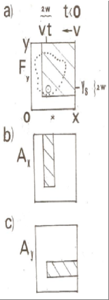
Figure 1: Non-zero regions of the functions appearing in this paper: shown by shading. (a) Regions of the phase function $F(x,y,t)$, equation (4). The tip of the source indicated by a circle and moving with a velocity $v(<0)$ is inside the $XY$ rectangle at times $X/v\leq t\leq 0$ and enters the box at a height of $y=Y_{s}$. $2w$ indicates schematically the function broadening. A domain with arbitrary shape is drawn with dotted lines. (b) Non-zero regions of the vector potential component $A_{x}$. (c) Same for $A_{y}$.

A vector potential functionally similar to that above, was used in [6]. The gauge dependence of $\vec{A}$ is nullified (for single valued gauges) by letting the source return to its initial position , rather than moving along a straight line, and considering the electronic state after return of the source to its starting position. In the present case an arbitrary gauge transformation can be applied to the Hamiltonian, together with a corresponding gauge factor in the wave function, without affecting the end result. In particular, one can work with a Coulomb gauge, equation (9). The reason of our preference for the vector potential description is that the references in the Introduction used this gauge, although with different forms for ${\vec{A}}$.

The present model takes us to a Hamiltonian:

$$H(x,y,t)=\frac{1}{2m}[(p_{x}-\frac{e}{c}A_{x}(Y_{s},t))^{2}+(p_{y}-\frac{e}{c}A_{y}(Y_{s},t))^{2}]+V(x,y)$$ (14)

where $V(x,y)$ is the potential confining the particle inside the rectangle of size $X-Y$.

Since the Hamiltonian is time dependent, electronic states $\Psi(x,y,t)$ will be obtained from the time dependent Schrödinger equation.

$$i\hbar\frac{\partial\Psi(x,y,t)}{\partial t}=H(x,y,t)\Psi(x,y,t)$$ (15)

We consider a solution whose initial form is fixed at the instant $t=X/v$, this being negative since $v<0$.

$$\Psi(x,y,t\simeq X/v)=\chi_{n_{x}}(x)\eta_{n_{y}}(y)$$ (16)

(cf. equation (3).) We now postulate the form for the state evolving adiabatically:

$$\Psi_{n_{x}n_{y}}(x,y,t)=e^{iQ(x,y,t)}\chi_{n_{x}}(x)\eta_{n_{y}}(y)$$ (17)

where

$$e^{iQ(x,y,t)}=e^{-iE_{n_{x}n_{y}}t/\hbar}e^{i\gamma_{n_{x}n_{y}}(t)}e^{i\frac{e}{\hbar c}F(x,y,t)}$$ (18)

As will emerge, the first factor is the dynamic phase factor (here appearing in a trivial form), the second is a geometric phase factor and the third factor is chosen, following [8], in order to eliminate the vector potential and the time dependence from the Hamiltonian through a gauge-transformation $U$ where:

$$U\equiv U(x,y,t)=e^{i\frac{e}{\hbar c}F(x,y,t)}$$ (19)

so that:

$$U^{-1}H(x,y,t)U\psi_{0}(x,y,t) =$$

$$H(x,y)\psi_{0}(x,y,t) \equiv \left[\frac{1}{2m}[p_{x}^{2}+p_{y}^{2}]+V(x,y)\right]\psi_{0}(x,y,t)$$ (20)

for any wave function $\psi_{0}(x,y,t)$. The $H(x,y)$ eigen functions are clearly of the form shown in equation (3). Substituting $\Psi(x,y,t)$ from equation (17) into the Schrödinger equation (15) and multiplying through with $e^{-iQ(x,y,t)}$one obtains

$$e^{-iQ(x,y,t)}i\hbar\frac{\partial[e^{iQ(x,y,t)}\chi_{n_{x}}(x)\eta_{n_{y}}(y)]}{\partial t} = E_{n_{x}n_{y}}\chi_{n_{x}}(x)\eta_{n_{y}}(y)+\delta_{n_{x}n_{y}}(x,y,t)$$ (21)

$$= H(x,y)\chi_{n_{x}}(x)\eta_{n_{y}}(y)$$

Thus, arising from the time derivative one has the leftover term

$$\delta_{n_{x}n_{y}}(x,y,t)=\left[-\hbar{\dot{\gamma}_{n_{x}n_{y}}(t)}-\frac{e}{c}\dot{F}(x,y,t)\right]\chi_{n_{x}}(x)\eta_{n_{y}}(y)$$ (22)

where the dot signifies time differentiation.

Expanding this expression in terms of the complete set $\chi_{m_{x}}(x)\eta_{m_{y}}(y)$, one sees that the first term in equation (22) has only ”diagonal” components ($m_{x}=n_{x},m_{y}=n_{y}$), while the second has both diagonal components, which will give the Berry phase [11], and non-diagonal components, which will be shown to be small in an adiabatic motion of the source.

Dealing first with the latter, we have for the absolute magnitude of the expansion coefficients arising from the second term only

$$|\frac{ev\Phi}{c}\int_{0}^{X}dx\chi_{m_{x}}(x)\chi_{n_{x}}(x)\delta_{s}(x-vt)\int_{0}^{Y}dy\eta_{m_{y}}(y)\eta_{n_{y}}(y)\Theta_{s}(y-Y_{s})|\leq$$

$$|\frac{ev\Phi}{c}|\int_{0}^{X}dx|\chi_{m_{x}}(x)\chi_{n_{x}}(x)|\delta_{s}(x-vt)\int_{0}^{Y}dy|\eta_{m_{y}}(y)\eta_{n_{y}}(y)|\Theta_{s}(y-Y_{s})\leq$$

$$|\frac{ev\Phi}{c}|[{\frac{2}{X}\int_{0}^{X}dx\delta_{s}(x-vt)}]\cdot[\frac{2}{Y}\int_{0}^{Y}dy|\Theta_{s}(y-Y_{s})]\leq$$

$$|\frac{4ev\Phi}{cX}|\cdot\frac{Y-Y_{s}}{Y}$$ (23)

for the non-trivial case that the source is inside the box ($Y_{s}\leq Y$). In going from the second to the third line we have inserted the forms of the functions from equation (3) and also noted that the sines are equal or less than unity. For the ${m_{x}m_{y}-n_{x}n_{y}}$ non-diagonal expansion coefficients to be negligible, these must be much less than the corresponding energy change, or

$$|\frac{4ev\Phi}{cX}|\cdot\frac{Y-Y_{s}}{Y}<<electronic~{}energy~{}differences=O(E_{n_{x}n_{y}})|$$ (24)

which is clearly satisfied in the adiabatic limit, with sufficiently low velocities $|v|$.

Turning to the diagonal part of the leftover terms, this vanishes provided:

$${\dot{\gamma}_{n_{x}n_{y}}(t)}=i<n_{x}n_{y},t|\frac{\partial}{\partial t}|n_{x}n_{y},t>$$ (25)

where the Dirac ket represents:

$$|n_{x}n_{y},t>\equiv e^{i\frac{e}{\hbar c}F(x,y,t)}\chi_{n_{x}}(x)\eta_{n_{y}}(y)$$ (26)

$\gamma(t)$ the time integral of this, is an overall phase of the wave function for all values of $t$ and, when $t$ is not a period of the source motion, is the ”Open path phase” [12]. As noted before, for $t=\tau$ the period in a cyclic motion of the source, $\gamma(\tau)$ is identified with the Berry phase. In the present context, it is a function of the vertical entrance position $Y_{s}$ (which appears in the phase function $F(x,y,t)$ of equation (4)). The Berry phase tends to cancel the acquired partial phases in the wave function, but achieves full cancellation only when the source motion fully encompasses the box [5]. To see this we elaborate on the full-period time integral of the right hand side of the above equation, as follows (dispensing, as we go along, with the wave function indices):

$$i\oint dt<n_{x}n_{y},t|\frac{\partial}{\partial t}|n_{x}n_{y},t>$$ (27)

$$= -\frac{ev\Phi}{\hbar c}\int_{X/v}^{0}dt\int_{0}^{X}dx[\chi(x)]^{2}\int_{0}^{Y}dy[\eta(y)]^{2}\Theta_{s}(y-Y_{s})\delta_{s}(x-vt)$$

$$= -\frac{ev\Phi}{\hbar c}\int_{X/v}^{0}dt[\chi(vt)]^{2}\int_{Y_{s}}^{Y}dy[\eta(y)]^{2}$$ (28)

$$= \frac{e\Phi}{\hbar c}\int_{0}^{X}d(vt)[\chi(vt)]^{2}\int_{Y_{s}}^{Y}dy[\eta(y)]^{2}$$ (29)

The equality after the first line is based on the fact that the chosen set vanishes outside the box. In equation (28) the first integration, over $vt$, covers the full $x-$ range of the confining box and therefore gives just $1$, but the second integration, over the truncated $y$-range, will be less than $1$, unless $Y_{s}\leq 0$, meaning that the source passes at the bottom edge of the box, or below. Thus equation (29) is generally less than the maximal AB phase. On the other hand, in the phase $\frac{e}{\hbar c}F(x,y,t)$ of the wave function, the part in which $x>|vt|$ and $y>Y_{s}$ (namely, above the source-motion line) gets the full AB phase and that in which $x<|vt|$ or $y<Y_{s}$ (below the source-motion line) gets no phase. Thus the Berry phase does not in general cancel the partial phases.

The solution to equation (15), with the proclaimed initial condition and insertion of the open path phase from the previous section, is that shown in equation (17). In the limit of an infinitesimally narrow source $(w\to 0)$, this wave function without the dynamic and open path factors has the following meaning:

The initial state is kept for source positions ”above” the box ($Y_{s}>Y$) or before reaching the box, but a phase is acquired if the source penetrates or is ”under” the box and then also only for that $x$-part (vertical section) of the wave function which the source has already passed. The overall phases which the adiabatic state acquires are the dynamic phase $-E_{n_{x}n_{y}}t/\hbar$ and the open path or Berry phase $\gamma_{n_{x}n_{y}}(t)$. There is no degeneracy in the system and, indeed, the energy $E_{n_{x}n_{y}}$ of the state not only does not coalesce with a neighboring one, but even stays constant during the source motion: an exceptional situation for adiabatic or any type of motion.

The described phase acquisition process , with the function-widths $w$ non-zero, is entirely continuous in that the region in which the new phase appears grows steadily from zero as the source enters the box from the right or from above and ultimately covers the whole box, which situation persists as the source passes the box from below.

Objection may be raised that in an adiabatic motion with a periodic Hamiltonian, at the completion of a period, the adiabatic wave function must return to its initial form except for an overall phase, whereas this is not the case for the adiabatic solution in equation (17) . However, this objection holds only for states that are not simultaneous eigenstates of the Hamiltonian, whereas the following proof shows that in the present case the wave functions obtained after an integral number of periods, although different, are co-degenerate solutions of the same Hamiltonian.

Proof (In the proof the coordinate dependence of the functions, as well as any overall time-dependent phase factor, are omitted, for brevity):

$\Psi_{n_{x}n_{y}}(t)=U(t)\chi_{n_{x}}\eta_{n_{y}}$ solves the periodic Hamiltonian $H(t)=H(t+\tau)$, $\tau$ being the period, with an eigenvalue $E_{n_{x}n_{y}}$ since

$$H(t)\Psi_{n_{x}n_{y}}(t) = U(t)U^{-1}(t)H(t)U(t)\chi_{n_{x}}\eta_{n_{y}}=U(t)H\chi_{n_{x}}\eta_{n_{y}}$$ (30)

$$= U(t)E_{n_{x}n_{y}}\chi_{n_{x}}\eta_{n_{y}}=E_{n_{x}n_{y}}\Psi_{n_{x}n_{y}}(t)$$

where $H$ denotes the time independent Hamiltonian in equation (20). We now show that the wave function $\Psi_{n_{x}n_{y}}(t+\tau)$ one period later, is also a solution with the same eigenvalue of the same Hamiltonian $H(t)$. (For $\tau$ not a period, the later wave function is a solution with the same eigenvalue, however, not of $H(t)$ but of a different Hamiltonian $H(t+\tau)$.)

$$H(t)\Psi_{n_{x}n_{y}}(t+\tau) = U(t+\tau)U^{-1}(t+\tau)H(t)U(t+\tau)\chi_{n_{x}}\eta_{n_{y}}$$

$$= U(t+\tau)U^{-1}(t+\tau)H(t+\tau)U(t+\tau)\chi_{n_{x}}\eta_{n_{y}}$$

$$= U(t+\tau)H\chi_{n_{x}}\eta_{n_{y}}$$

$$= U(t+\tau)E_{n_{x}n_{y}}\chi_{n_{x}}\eta_{n_{y}}=E_{n_{x}n_{y}}\Psi_{n_{x}n_{y}}(t+\tau)$$

where in going from the first to the second line we have used the periodicity of the Hamiltonian.

Thus, after one full cycle the wave function turns, instead of the initial state, into a co-degenerate state, different from but not orthogonal to the initial one. If the AB phase is a rational submultiple of $2\pi$, each further cycle will bring the system to a new co-degenerate state, until the accumulated phases add up to $2\pi$ (or its integral multiple), i.e. the initial state is regained.

It should also be noted that this ”periodicity-degeneracy” involving all wave functions differing by a multiple of the trajectory period is unrelated to the degeneracies found at discrete values of the solenoid coordinates in [8].

In conclusion, we have considered the adiabatic penetration into a spatially extended electron by a source, which is such that there is no magnetic field, only a weak, motion-induced electric field. A distributed (i.e., not overall) phase acquisition by parts of the electron occurs, and agglomerates in the course of continued cyclic motion. A remarkable feature of this outcome is that whereas , in the limit of extreme adiabaticity, the electric field is too weak to cause energy excitations, the vector potential does change the phases (differentially and locally). This resembles some analogous features in the AB and Berry’s phase effects (no fields and still phase change). Indeed the present result can be formulated as a weakened AB effect, in that a measurable phase acquisition by the vector potential alone occurs in regions where there is no magnetic field and the electric field, though not nil, is so weak that it causes no excitation or admixture.

The novelty in this letter’s time dependent treatment, compared to [2]-[8], is the absence of local degeneracies and the phase acquisition by parts of the wave packet. These results carry over to generalizations regarding forms of the confining box illustrated by dotted lines in Figure 1 (a) and of vector potentials derived from arbitrary forms of the phase functions, subjects that will be treated in the future. Future study will also consider many particle effects, resulting in specific braiding properties, e.g., the acquisition by the many particle wave-function of a non-integral $\pi$ phase upon adiabatic interchange of two neighboring particles.

References

- [1] 9
- [2] BERRY M. V. and WILKINSON M., Proc. Roy. Soc. London A 392 (1984) 15
- [3] BERRY M.V. and ROBNIK M., J. Phys. A 19 (1986) 644, 1365
- [4] MONDRAGON R.J. and BERRY M.V. , Proc. Roy. Soc. London A 424 (1989) 263
- [5] REZNIK B. and AHARONOV Y., Phys. Lett. B 315 (1993) 386
- [6] AHARONOV Y. and KAUFHERR T. , Phys. Rev. Lett. 92 (2004) 070404
- [7] AHARONOV Y., COLEMAN S., GOLDHABER A. , NUSSINOV S., POPESCU S., REZNIK B. , ROHRLICH D. and VAIDMAN L. , Phys. Rev. Lett. 73 (1994) 918
- [8] BERRY M.V. and POPESCU S., J. Phys. A: Math. Theor. 43 (2010) 354005 doi:10.1088/1751 - 8113/43/354005
- [9] POPESCU S. , ”Dynamic Non-locality and the Aharonov-Bohm Effect” A presentation at the ”50 years of the Aharonov-Bohm Effect, Concepts and Applications” symposium at Tel Aviv University, (Tel-Aviv, October 2009)
-
[10]
A closed, periodic trajectory of the source describing a large square frame of perimeter length can be incorporated
in the formalism by rewriting the phase function in equation (4) in terms of the moving source coordinates
by and defining six
times , at which the phase function changes
Along its trajectory the source coordinates are given in the time interval by the compact (though complicated looking) expressions:(32)
The trajectory is periodic, in that at the source is at the same position as it was at a time-period earlier, namely at . Generation of the phase occurs only in the time interval (if the small width is disregarded). Subsequent periodic trajectories can be similarly incorporated in the formalism. For these one has to interpret in the phase function modulo . However, so as to ensure the continuity of the wave function, in the transformation equation (19) one has to add Integer to the phase. Thus, the phase increases smoothly with each cycle.(33) - [11] BERRY M.V. , Proc. Roy. Soc. London A412 (1984) 45
- [12] BHANDARI R. , Phys. Rev. Lett. 89 (2002) 268901