Local Theory of Holomorphic Foliations and Vector Fields
Foreword
These notes constitutes a slightly informal introduction to what is often called the theory of (singular) holomorphic foliations with emphasis on its local aspects that may also be called singularity theory of holomorphic foliations and/or vector fields. Though the text is unpolished, we believe to have provided detailed proofs for all the statements given here. The material is roughly split into two parts, namely Chapters 1 and 2. Chapter 1 is primarily devoted to motivation for the theory of “(singular) holomorphic foliations” and in this direction it contains several examples of these foliations appearing in situations of interest. It also contains some general background from analytic geometry and topology that are often used in their study. This chapter is essentially of global nature so its purpose is indeed to motivate (and to provide some for) the study of globally defined foliations/differential equations rather than the study of their singularities that is the object of Chapter 2. Explanations for this discrepancy begin by saying that these notes are planned to be continued in the future with the inclusion of new chapters. Besides it is interesting to point out that the (local) study of singularities already entails a global perspective once the dimension of the ambient is at least . The simplest way to notice the existence of global foliations (possibly with rather complicate dynamics) hidden into the structure of a singularity of a vector field defined on, say, , is to perform the blow-up of the singularity in question (cf. Section 1.4.1). In general, the blown-up foliation will induce a globally defined foliation on the resulting exceptional divisor (isomorphic to the complex projective plane in this case). Actually this foliation depends only on the first non-zero homogeneous component of the Taylor series of the mentioned vector field. Besides all foliations on the projective plane are recovered in this way, see “Example 3” in Section 1.3.
Chapter 2 is then devoted to the singularity theory for vector fields/foliations. Most of the chapter is taken up by the case of singularities defined on where the theory has reached a high level of development, with landmark progresses being represented by the papers of Mattei-Moussu and of Martinet-Ramis, [M-M], [Ma-R]. Much of this chapter is indeed devoted to present the results of these papers. Yet we have also included some classical and more recent material concerning singularities in higher dimensions.
In a sense these notes are vaguely reminiscent from a course the first author lectured at Stony Brook several years ago. He would like to thank the audience of his course and specially Andre Carvalho and Misha Lyubich for their interest. The project of writing these notes, however, would never be undertaken if it were not by the interest of Gisela Marino to whom we are most grateful. Gisela was the first to put into typing and fill in details of definitions and proofs for most of what is now “Chapter 2”, cf. [Mr]. Unfortunately she did not wish to continue her study and left to us to complete the present material (as well as the planned subsequent chapters).
The authors
Chapter 1 Foundational Material
We are interested in understanding the behavior of first order ordinary differential equations in , where the “time” parameter is in .
To begin with, let us recall the main aspects of real ordinary differential equations. Complex Ordinary Differential Equations (ODEs) can then be obtained from real ones from a natural “complexification” procedure. It will be seen that complex ODEs are closely related to singular holomorphic foliations.
1.1 Real Ordinary Differential Equations
Let be a vector field given by , where and are polynomials. The ordinary differential equation associated to this field is:
It can also be regarded as the following system of ODEs
| (1.1) |
Since the vector field is sufficiently smooth (, in fact) we may assert that given a and , there exists a unique solution of (1.1) defined on a neighborhood of , and verifying
Furthermore, there exists the concept of extending a local solution to obtain a solution defined on a maximal domain, i.e, on the “largest possible interval”. This means that for each there exists an interval and a solution of (1.1) defined on which satisfies the following conditions:
-
1.
-
2.
If defined on , , is another solution of (1.1) verifying , then, and, furthermore, .
Let be the open set . The flow associated to (1.1) is defined to be:
where is the solution of (1.1) such that .
Notice that the flow may not be complete. That is, it may not be defined for all , since is not necessarily the whole real line. On the other hand, it is easy to check that, when then tends to infinity as approaches the extremities of , for a fixed . Here we say that “tends to infinity” in the sense that it leaves every compact set contained in the domain of definition of .
Remark 1.1
The above discussion actually holds for every regular (say ) vector field on arbitrary manifolds. Also it is well-known that, if the orbits of a regular vector field are contained on a compact set, then the maximal interval of definition for the corresponding solutions is, indeed, . In other words the flow generated by this vector field is complete. In particular every regular vector field defined on a compact manifold (without boundary) is complete.
Let us now return to our polynomial vector field . What precedes implies that the image of decomposes into a set of curves (orbits of ) along with the singular points of . To develop this remark further, let us recall the definition of (regular, real) foliations.
Definition 1.1
Consider a manifold of real dimension . A foliation of class and of dimension on consists of a distinguished coordinate covering , , of satisfying the conditions below:
-
1.
If , then , where are open discs of and respectively.
-
2.
If and , then the change of coordinates has the form where and .
Naturally a distinguished coordinate covering for a foliation can automatically be enlarged to a maximal foliated atlas. A distinguished coordinate is sometimes called a foliated chart, a foliated coordinate or even a trivializing coordinate for . Given a foliated chart as above, a set of the form is called a plaque. A plaque chain is a sequence of plaques such that for every . We then introduce an equivalence relation between points of by stating that is equivalent to if there is a plaque chain such that and . The classes of equivalence of this relation are said to be the leaves of .
Remark 1.2
If is a complex manifold and the changes of coordinates for a foliated atlas are, in fact, holomorphic diffeomorphisms then we have a holomorphic foliation.
With this terminology, we return to the vector field . A standard fact about Ordinary Differential Equations is the so-called Flow Box Theorem. It states the existence of a diffeomorphism defined on a neighborhood of a non-singular point of , such that , where denotes the canonical basis of . Once again, this result holds for vector fields () and the resulting diffeomorphism has the same regularity of the vector field.
In particular, away from the singular points of , the Flow Box Theorem implies that solutions of ODEs are the leaves of a foliation of dimension . In this sense, we say that the image of defines a singular foliation on . We shall make this definition more formal in the sequel.
1.2 Complex Ordinary Differential Equations
We now wish to extend these notions to the complex case. The main idea is to identify with by considering a complex structure on . To do this, we must define an automorphism of that plays the role of the multiplication by in a complex vector space. More precisely, a complex structure on consists of an automorphism satisfying . In the sequel we are going to use the “standard” complexification, where is given by .
Now, let given by be a polynomial vector field. The complex ODE associated to this field is
| (1.2) |
where the time parameter is complex. Once again, being a holomorphic vector field, the complex version of the Theorem of Existence and Uniqueness for regular ODEs guarantees that given and there exists a unique holomorphic solution of (1.2) defined on a neighborhood of , and satisfying:
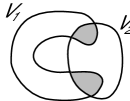
The next step would be to try to glue together these local solutions so as to obtain a “maximal domain of definition”. However we notice that, in general, this is not possible since the time parameter is in . Indeed, the problem is that, as we try to glue together the neighborhoods, their union may not be simply connected (see figure below). Consequently, the solution may not be well-defined on all of , i.e, it may be multi-valued. This is an important difference between real and complex ODEs. This phenomenon is illustrated by Figure (1.1), since the intersection of and is not connected, solutions defined on and cannot, in general, be “adjusted” to coincide in both connected components.
Let us now introduce a more geometric point of view for these topics. Using the above mentioned identification of with (and with ), a solution of (1.2) starting at may be regarded locally as a “piece” of real -dimensional surface in passing through the point . In addition, at , is tangent to the vector space spanned by the vectors
| (1.3) |
where is regarded as a real map from to , and () satisfies the Cauchy-Riemann equations. Notice that is invariant under the automorphism , due to the Cauchy-Riemann equations, so that is indeed a complex line, i.e the image of a one-dimensional subspace (over ) of under the preceding identification.
As the initial conditions vary, from (1.3) we obtain a distribution of -real dimensional real planes (or complex lines) that can be integrated in the sense of Frobenius to yield -dimensional surfaces (or complex curves). In particular, away from its singular set, the vector field defines a foliation of real dimension equal to . Furthermore this foliation is holomorphic as it follows from the complex version of the Flow Box Theorem.
The leaves of the foliation in question inherit a natural structure of Riemann surfaces. Actually an atlas for this structure is provided by the local solutions of (1.2). More precisely, is a holomorphic diffeomorphism from to its image in the leaf (Riemann Surface) .
Summarizing what precedes, a holomorphic vector field on immediately yields a holomorphic foliation on away from its singular set. Again we also say that the vector field defines a singular foliation on which is said to be its associated foliation (or underlying foliation). Conversely, given a (singular) holomorphic foliation , in order to obtain the vector field whose non-constant orbits are the leaves of , we need an extra data. More precisely, we must associate a complex number (or vector in ) to the tangent space of each leaf, so as to recover the parametrization of the leaves of , which in the above situation was given by . This complex number will be playing the role of the “speed” of the flow of . It allows us to recover the local parametrizations for the leaves of the foliation which are given as local solutions of (1.2).
Clearly the notion of singular holomorphic foliation is a convenient geometric way to think of a complex ODE (equivalently a holomorphic vector field). Nonetheless the above remark shows that it does not capture all the information contained in a vector field. As already mentioned, the local solutions in general cannot be glued together and this makes the problem of extending them, as far as possible, more subtle. We shall return to this problem later.
1.3 Basic Definitions and Examples
After the relatively informal discussion of the previous section, we shall now begin to provide precise definitions and detailed statements.
Definition 1.2
A complex manifold of dimension is a differential manifold equipped with an atlas such that:
is holomorphic whenever , and , .
By virtue of the Cauchy-Riemann equations, the Jacobian determinant of a holomorphic diffeomorphism is always positive. It then follows that every complex manifold is orientable.
The Cauchy-Riemann equations also imply that a map is holomorphic if and only if , for . So that vectors in invariant under are sent by to vectors that are invariant under as well. In other words, if is holomorphic then preserves -dimensional complex planes.
Next, we shall give a working definition of singular holomorphic foliation on a complex manifold which is going to be used throughout these notes.
Definition 1.3
A singular holomorphic foliation defined on a complex manifold consists of the following data:
-
1.
There exists an atlas compatible with the complex structure on , where .
-
2.
There exist holomorphic vector fields defined on each , given by .
-
3.
If then there exist functions such that:
When is a complex surface (i.e. has complex dimension ), we have initially thought of singular foliation as being a regular foliation defined away from finitely many points (the corresponding singularities). In this regard the definition above seems to be more restrictive. Yet this is not the case.
If the functions are actually all constant and equal to , then we have, indeed, a holomorphic vector field on .
Definition 1.4
A holomorphic vector field defined on a manifold is such that, given an atlas of , , the following equation is satisfied:
where and are as in Definition 1.3.
In the sequel we present a list of vector field and foliations of varied nature. Our main purpose is to convince the reader of the richness and importance of the subject. The first elementary examples will also give us a hint that the condition required to define a vector field on a complex manifold is much stronger than the conditions that allow us to define a singular holomorphic foliation.
Example 1: Complex Tori
Let be a lattice on . The -dimensional complex torus is the quotient space . Notice that a constant vector field on induces a holomorphic vector field on the torus. In fact, constant vector fields are obviously preserved by the translations of associated to the elements of . Thus descends as a holomorphic vector field to the torus given by the quotient .
Example 2: Hopf Surfaces
Consider , in such that and . Let . The Hopf surface associated to is the quotient . It is immediate to check that is, in fact, a complex -dimensional manifold.
Let be a polynomial vector field on such that
where . Then defines a singular holomorphic foliation on . The reader will notice, however, that in order to obtain a holomorphic vector field in the Hopf surface, one should have the above ratio equal to . This indicates that in Hopf surfaces, there are many more holomorphic foliations than holomorphic vector fields.
The following concrete example illustrates this. Let and . Consider the polynomial vector field given by where:
Notice that
On the other hand,
so that . In view of the above discussion, the vector field induces a holomorphic foliation on but not a holomorphic vector field.
Example 3: Complex Projective Plane (Space)
Foliations on complex projective spaces constitute the main source of examples, in the sense that they are easy to describe and, in addition, they usually already encode the essential difficulties of more general cases. For this reason, they are going to be treated here with a significative amount of details. Let us begin by considering the following relation of equivalence:
The equivalence classes form the -dimensional complex projective space, denoted by .
Two points define the same point in if and only if
so that the projection is determined by the ratios between the coordinates of . Traditionally is denoted by and are called homogeneous coordinates for .
Let us consider the following open sets that cover :
Along with these open sets, we have the following coordinate charts:
Now let . A direct inspection using the coordinate charts introduced above shows that is isomorphic to . Thus i.e. may be regarded as being added to the Riemann sphere. In this sense is a compactification of . Moreover in the affine coordinates , corresponds to “infinity” and is linearly embedded in . For these reasons it is called the line at infinity. Finally, we note that this construction applies to any affine coordinates in , that is, any affine gives rise to a “line at infinity”.
We will construct singular holomorphic foliation on in a similar way to what was done in the case of Hopf surfaces.
Let us consider a homogeneous polynomial vector field on of degree . Consider the action of on given by the homotheties , . As already pointed out, the quotient of this action is precisely . On the other hand, note that
Besides,
Therefore so that “the directions” associated to are invariant under homotheties. Hence indeed defines a singular foliation on .
Another equivalent way to define a singular holomorphic foliation in is to consider a polynomial vector field in and see that it can be extended to an holomorphic foliation on all of . Details are provided below.
In fact, it can be shown that every holomorphic foliation in is induced by a polynomial vector field in .
Let be a polynomial vector field in the affine coordinates . Naturally, it induces a rational vector field (resp.) defined on the affine coordinates (resp. ). Then we only need to multiply the vector fields by their denominators so as to have holomorphic ones (indeed polynomial ones).
For example, is given by:
As already mentioned, this vector field is not holomorphic in the domain of the coordinates since it has poles over . However, multiplying by , the new vector field is obviously holomorphic (and with isolated singularities) in the domain of . Now changing from the coordinate system to one obtains
Repeating this procedure with the other coordinate charts, we obtain a holomorphic foliation on . Finally note also that the original polynomial vector field on does not induce a holomorphic vector field on . Instead it induces a meromorphic vector field whose poles are contained in the corresponding line at infinity.
This has an obvious generalization to higher dimensional complex projective spaces which is left to the reader.
We have constructed singular holomorphic foliations on following two a priori different methods:
-
•
By means of a homogeneous polynomial vector field on .
-
•
By means of a polynomial vector field on .
It is easy to check that both constructions are equivalent in the sense that they produce the same set of foliations. This verification is implicitly carried out in the proof of Lemma (1.2). It is however much harder to show that these constructions give rise to all singular holomorphic foliations on . This is the contents of Theorem (1.1) below.
Theorem 1.1
Let be a singular holomorphic foliation on . Then there is is induced by a homogeneous polynomial vector field on which, in addition, has singular set of codimension at least .
In view of Theorem (1.1), it is natural to try to define a notion of degree for a foliation on . At first, one might feel tempted to define it as the degree of a polynomial vector field representing the foliation in affine coordinates. However, as the reader can easily verify, this degree may, in fact, vary depending on the affine coordinates chosen.
The following lemma will motivate the correct definition of the degree for a foliation on induced by a polynomial vector field on . Let and where , are homogeneous polynomials of degree .
Lemma 1.1
The “line at infinity”, , of is invariant under the foliation , induced by as above, if and only if the top-degree homogeneous component is not of the form , for some polynomial of degree .
Proof. To understand the behavior of near infinity in the coordinate system , we use the following change of coordinates: , . So that this vector field in the coordinate chart is given by:
and now we only need to analyze the corresponding foliation on a neighborhood of .
Let us denote by , and by . Notice that , for appropriate polynomials and of degree . Also, , naturally there is an analogous expression for . Multiplying the vector field by we obtain a holomorphic vector field in the -coordinate which is given by
where .
Now, if , the components of are both divisible for . By eliminating this common factor, it becomes clear that the line at infinity is not preserved by the foliation. Conversely, if is not identically zero, is preserved, since the component of vanishes identically over .
Finally it is clear that vanishes identically if and only if the top-degree homogeneous component is radial.
Definition 1.5
The degree of a foliation on given by the compactification of the polynomial vector field of degree and having only isolated zeros is equal to:
-
1.
, if there exists a polynomial of degree such that . In other words, if the top-degree homogeneous component of is a multiple of the radial vector field.
-
2.
, otherwise.
It should be verified that this is indeed well-defined.
Here we shall give a more geometric interpretation of the degree of a foliation as defined above. In fact, the contents of this lemma can be used as an equivalent definition of degree.
Lemma 1.2
Let be a singular holomorphic foliation on of degree . Then the following holds:
-
1.
There is a homogeneous polynomial vector field of degree on , with singular set of codimension at least , which induces by radial projection of its orbits;
-
2.
The number of tangencies of with a generic projective line is .
Proof. Let us first show that the projection of the foliation associated to a homogeneous polynomial vector field of degree on is, indeed, a foliation on having degree . Let , where stands for the coordinates of . In the chart , the vector field becomes
If has degree (i.e, is not divisible by ), then has degree . Furthermore, the top-degree component of is given by , where stands for the homogeneous component of degree of . So, according to Definition (1.5), has degree .
If has degree less than (i.e, is divisible by ), then at least one between and must have degree , otherwise all of the three polynomials would be divisible by . This would mean that the singular set of has codimension , which contradicts our assumption. Therefore, has degree , and once again Definition (1.5) implies that has degree . The converse is analogous and establishes the first part of the statement.
Let us now consider the tangencies between and a generic line in . Modulo performing a projective change of coordinate, we may suppose that the tangencies with a generic projective line are all contained in the main affine chart of so that they are given by:
that is, by the zeros of the polynomial . Hence the number of tangencies (counted with multiplicity) is the degree of . However, if is the degree of the foliation, then either is radial (and consequently has degree ) or it is not (and has degree ). The first case is equivalent to have , which means that has degree . The other case only happens when the top-degree component of is not zero, implying that the degree of this polynomial is . The converse is again analogous.
According to Theorem (1.1) and to Lemma (1.2), the space consisting of singular holomorphic foliation of degree is naturally contained in the space of homogeneous polynomial vector fields of degree on three variables. Besides two such vector fields having a singular set of codimension at least define the same foliation if and only if they differ by a multiplicative constant. Thus a simple counting of coefficients yields the following corollary:
Corollary 1.1
The space is naturally identified with a Zariski-open set of the complex projective space of dimension
It should also be noted that the group of automorphims of , , has a natural action on through projective changes of coordinates.
Example 4: Foliations on weighted projective spaces
This is a very natural generalization of the previous example that often appears in higher dimensional questions related to resolution of singularities, cf. for example [A]. They are also similar to foliations on Hopf surfaces.
A polynomial on variables is said to be quasi-homogeneous with weights and degree if and only if for every one has
For example is not only quadratic (ie homogeneous of degree ) but also quasi-homogeneous of degree relative to the weights .
Chosen a set of weights , we have a natural action of on given by
Consider the quotient space of where two points are identified if and only if they belong to the same orbit of . The resulting space is a compact manifold with singularities called a weighted projective space whose dimension is obviously equal to . Whether or not it actually has singularities, this type of manifold can be given an algebraic structure since it can be realized as a Zariski-closed set of a complex projective space with sufficiently high dimension. The existence of this imbedding can easily be shown by means of Plücker coordinates.
Alternatively the quotient of this -action can also be realized as the quotient of the projective space of dimension by some finite group of automorphism.
Next a polynomial vector field is said to be quasi-homogeneous with weights and degree if and only if for every one has
where stands for the map . An example of quasi-homogeneous vector field with weights and degree is
If is quasi-homogeneous with weights then the definition above implies in particular that unequivocally defines a complex direction at each point of the projective space with the same weights . Being of complex dimension , these directions can naturally be integrated to form a singular holomorphic foliation. Therefore quasi-homogeneous vector fields give rise to singular holomorphic foliations on weighted projective spaces.
Example 5: Riccati Foliation The classical Riccati equation is given by
where are complex variables. We are interested in the case where are rational functions of . In this case, if denotes the least common multiple of the denominators of , the preceding equation is equivalent to the vector field
with polynomials. Although it is possible to compactify the associated foliation on , it is more natural to compactify it in . Consider the “vertical” projection onto the first factor. The change o coordinate allows one to check that the vector field has a holomorphic extension to the “infinite” of the fibers (or to the section at infinity). However has in general poles on the “fiber over infinity” of affine coordinates . In the initial affine coordinates , we see that the set is consituted by invariant fibers and contains all the (affine) singularities of the underlying foliation . A similar calculation applies to the fiber over infinity. Thus we conclude that the foliation associated to has the following properties:
-
1.
It admits a nonzero number of invariant fibers given in the affine coordinates by . The fiber over infinity may or may not be invariant by this foliation.
-
2.
The union of these invariant fibers contains all the singularities of .
-
3.
Away from the invariant fibers, is transverse to the fibers of .
Since the fibers of are compact, a simple remark due to Ehresmann guarantees that the restriction of to the regular leaves of (different from the invariant fibers) defines a covering map onto where are precisely the projection of the fibers invariant under .
Fix a fiber , with . Thanks to the remark above, paths contained in can be lifted in the leaves of . Therefore we can consider the global holonomy of (w.r.t. ). This is given by a homomorphism
Since is isomorphic to , the homomorphism can also be viewed as taking values in this latter group. In particular the theory of the Riccati equations is naturally connected to the theory of finitely generated subgroups of . In particular, in the cases where the group is in addition discrete, to the theory of Kleinian groups and consequently, at least to some extent, to hyperbolic geometry in dimension . We also note that, conversely, a classical result due to Birkhoff states that every finitely generated subgroup of can be relized as the monodromy group of some Riccati equation. As a matter of fact, this correspondence is not unique: there are several Riccati equations possessing the same monodromy group. This raises the question of trying to find the “simplest” Riccati equation realizing a given monodromy group. As far as we know, this question has not been addressed to in the literature.
Example 6: Linear Equations
Linear equations are among the most classical topics in complex analysis. They generalize Riccati equations as well as many other equations such as Gauss hypergeometric equation, Fuchsian equations and so on. Furthermore they play a significative role in the theory of vector bundles over Riemann surfaces.
In a classical setting we consider a meromorphic function from with values on , for some . These are simply a family of invertible matrices of rank whose coefficients are meromorphic functions defined from to . The notion of invertible matrices of course refer to those points away from the poles of these coefficients.
Example 7: Jouanolou Foliation
This is a very special example of foliation on the complex projective plane. Fixed , the Jouanolou foliation of degree is the foliation induced on by the homogeneous -form
The reader will notice that the kernel of always contains the radial direction so that it naturally induces a line field, and hence a foliation, on . In terms of homogeneous vector field, the foliation is given by
In standard affine coordinates, , the foliation is induced by the vector field
The main result of Jouanolou states that leaves no algebraic curve invariant. Foliations leaving algebraic curves invariant will be discussed in detail in Chapter 3 and the foliations will play a significative role in the discussion. For the time being, let us only mention some elementary properties of . The proofs of the assertions below amount to direct inspection in the spirit of the preceding example, they are therefore left to the reader.
We begin by noticing that is left invariant by a nontrivial group of automorphisms of . To identify this group, let be a primitive -root of the unit with . The cyclic group generated by the automorphism preserves as well as it does the group generated by the cyclic permutation . The order of is precisely while the order of is obviously equal to . It can be checked that and generate the maximal group of automorphisms of preserving .
It is a remarkable fact that all the foliations , , are obtained by means of a family of quadratic foliations on . This can be done as follows. Consider that map given in homogeneous coordinates by . This induces a ramified covering of with degree . It can be checked that is the pull-back where is the quadratic foliation on induced by the homogeneous vector field
The reader will immediately check that has exactly singularities. These correspond to the radial lines invariant by , namely the coordinates axes, , , and where . also leaves projective lines invariant, namely those induced by projection of the coordinates -planes. It is easy to see that the lines form a “triangle” containing the singularities of except for the singularity . This “triangle” is the “maximal” algebraic curve invariant by .
Naturally is still invariant by the permutation , and hence by the group . It is therefore possible to further “simplify” by exploting these symmetries. This would lead us to a foliation of higher degree leaving a single irreducible algebraic curve invariant. Further information on Jouanolou foliations can be found in Chapter along with some specific references.
Example 9: Ramanujan Differential Equation
This is a system of differential equations introduced by Ramanujan that plays a significative role in the part of Number Theory dealing with transcendent numbers. The system closed related to the following vector field defined on .
This vector field is, indeed, a particular example of class of differential equations known as Halphen vector fields. These were detailed studied by A. Guillot in [Gu]. In later chapters, we shall have occasion to talk more about Halphen vector fields. For the time being, we would like to indicate very briefly the connection between the above vector field and the theory of transcendent numbers, for further information we refer the reader to [Ma-Ro]. This begins with the so-called Ramanujan functions that can be defined by explicit formulas as follows.
where and , ie is the sum of the -powers of the positive integers dividing . Since these formulas may look especially weird, let us mention that they can be obtained from rather natural procedures with automorphic functions. For our present purpose however the above definition will suffice. For example, it makes easy to see that these functions are defined for . It is less easy to see that the unit circle constitutes an “essential boundary for them” in the sense that the have no holomorphic extension to a neighborhood of any point in the circle. The interest of these functions for number theorists is partially due to the fact that they assume “specially remarkable values” for specific choices of .
According to Ramanujan, the functions verify the following nonautonomous system of differential equations:
Although this system is not autonomous, it ensures that the “velocity vector” of the parametrized curve is parallel to at the point . In other words, this curve parametrizes a leaf of the foliation associated to . Actually, the image of this curve also contains the point that technically speaking does not belong to the leaf in question since is a singular point of .
If we choose (for example ) and the corresponding point , we can compare the functions with the actual solutions of the vector field satisfying the initial value condition . This would lead us to the simple (-dimensional) equations , and . Therefore the solutions are
Naturally the effect of changing the initial data and essentially amounts to performing a translation for the functions and thus is of little importance.
Summarizing the preceding discussion, we conclude that information on the properties of can be extract from the study of the solutions of the vector field .
Example 10: The Lorenz Attractor
In the course of the past few years, the dynamical system associated to Lorenz attractor has become a paradigmatic example of “chaotic dynamics”. The vector field defining the dynamical system was introduced by Lorenz in [L] in connection with a evolution problem for atmospheric conditions. In general, the domain belongs to fluid dynamics and the phenomenon is governed by the KdV equation. Since these equations are notoriously hard to be analysed, Lorenz thought of his vector field as a simplified model to describe this evolution. The vector field in question is simply given by
It is therefore a quadratic vector field (obviously is not homogeneous so that “quadratic” here is a abuse of language) defined on . Despite its innocent appearance, exhibits a remarkably complicated dynamics. A traditional picture of the plotting of orbits of looks like figure 1.2.

Figure 1.2 seems to indicate the presence of an “attractor” for . The definition of the term “attractor” may vary depending on the context and we shall give none in this discussion. In any case the guiding picture to bear in mind is that of a “compact invariant set” attracting nearby orbits. In particular, orbits of points that actually belong to the attractor remain contained in it forever (both in “past” and in “future”). Since this attractor is not hyperbolic, it was called “strange”. Here the reader may consider that hyperbolicity is the best known mechanism to produce this type of behavior. Besides, it has been established that the attractor, if it existed, was robust, ie. it could not be destroyed by performing a small perturbation on . Curiously enough, the very existence of Lorenz attractor was settled only recently by W. Tucker through rigorous numerics [T]. An interesting survey on the Lorenz attractor containing in particular precise definitions and notions is [V]. For a beautiful geometric discussion of the properties of this attractor, including some wonderful graphics, the reader is referred to [G-L].
Although the interest on Lorenz vector field has primarily to do with its real dynamics, this vector field can equally well be thought of as being a complex polynomial (and thus holomorphic) vector field defined on . It is natural to consider this complexification not only for it may provide new insight in the real dynamics, but also because it is likely to be interesting in itself. Besides, in view of Example 3, it may be useful to consider the holomorphic extension to of the foliation associated to .
Elementary calculations yield some basic facts, such as singularities and existence of invariant curves, about viewed as a singular holomorphic foliation on . In the affine , the foliation has exactly three singularities corresponding to the points , and which in addition have non-degenerate linear part. Also the axis is obviously invariant by . The plane at infinity is also invariant by and contains other singularities of it. In coordinates , and , the plane at infinity is given by the restriction of to this plane coincides with the one induced by the vector field . In particular, it has a singularity whose eigenvalues vanish at . The complement of the coordinates in is a projective line that is, in addition, invariant by . This line contains the last two singularities of .
The picture of the existence of the Lorenz attractor and the consequently existence of real orbits lying entirely in some compact set of raises the question of knowing if a similar phenomenon will happen with the complex leaves of . This is however not the case. Still the question serves as motivation for us to state and proof Proposition 1.1 below. This proposition will play a significative role in Chapter 4 as well as it does in many aspects of the study of holomorphic foliations on complex projective spaces.
Proposition 1.1
Let be a holomorphic foliation of and consider the foliation obtained as the restriction of to an affine . Then no regular leaf of can entirely be contained in a compact set .
It is to be noted that this proposition cannot be derived as an immediate consequence of the maximum principle since the orbits of need not be compact. Indeed, in the compact case, we can consider the projection of the compact leaf on a chosen coordinate and argument that the image of this projection must be a single point by virtue of the maximum principle. In fact, there must be a point in the leaf corresponding to a projection of “maximal modulus”. It then follows that the projection in question is constant. In the case of open leaves, it is not obvious that the maximum of a projection as above is attained so that we cannot conclude that the projection is constant.
Proof. Suppose for a contradiction that is a regular leaf of that is wholly contained in a compact set . Consider a polynomial vector field tangent to . The leaf of can then be considered as an orbit of . Since is uniformly bounded in , there exists such that for every the solution of satisfying the initial condition is defined on a disc of radius about . Now we proceed by choosing a point and considering the solution satisfying , for some . Naturally is defined on the disc of radius about . Next consider a point in the boundary of . Modulo reducing from the beginning, we can without loss of generality suppose that . However must belong to so that the solution of satisfying is defined on the disc of radius about . Since the union is simply connected, it follows from the monodromy theorem that the solutions can be patched together into a solution of defined on . Actually, since is arbitrary in the boundary of , it follows that this boundary can be covered by finitely many discs as indicated above. By repeatedly using the monodromy theorem, we conclude that the initial solution , , can be extended to a disc of radius about with uniformly chosen. An obvious induction shows that this solution is defined on the disc of radius about for every . In other words, is defined on all of .
The desired contradiction follows now from Liouville Theorem: since is a bounded holomorphic map from to it must be constant. The proposition is proved.
1.4 Basic tools
1.4.1 The Blow-up of manifolds and of foliations
At first sight, the “blow-up” may be thought as a device that simply creates new manifolds out of previous ones. However, it will be seen that it is particularly useful to understand the behavior of foliations or vector fields at singular points.
Definition 1.6
The blow-up of at is a complex manifold obtained by identifying two copies of in the following way:
where and are the coordinates of the two above mentioned copies.
By definition, the exceptional divisor of is given by (resp. ) in the coordinates (resp. ). Therefore is well-defined and it is isomorphic to .
The blow-up mapping is given by and . Moreover, it verifies the following:
-
•
;
-
•
is a holomorphic diffeomorphism;
-
•
is proper (i.e. the preimage of a compact set is also compact).
Now we shall define the blow-up of a complex -dimensional manifold at a point . Consider a local coordinate chart defined on a neighborhood of and such that .
Let , where is the blow-up mapping. Let be the disjoint union of with , and consider the following equivalence relation:
The blow-up of at is the quotient . Notice that is indeed a smooth complex manifold for is a manifold and is a holomorphic diffeomorphism.
Similarly, there is a blow-up mapping from to (which will also be denoted by ) that is proper and takes to , i.e. . Moreover, is a holomorphic diffeomorphism.
The blow-up of a foliation or vector field can also be defined in a natural way. Let be a vector field on a neighborhood of the origin in , where and are holomorphic functions. Suppose that is a singularity of of order ( is the minimum between the orders of and at ).
Let , and , where and are the homogeneous components of degree of the Taylor series of and , respectively.
By using the blow-up mapping in the coordinates, namely (), has a natural meaning. In fact, one has
Setting and , the above equation becomes
| (1.6) |
It is to be noted that this vector field admits a holomorphic extension to (). Thus, is defined to be the blow-up of at the singular point . Moreover, if then is singular at every point of . Similarly, the blow-up of the foliation associated to is the foliation associated to .
The behavior of (and of ) on a neighborhood of is significantly different, depending on whether or not is identically zero. Let us analyze each case separately.
-
•
If is not identically zero.
Dividing Equation (1.6) by , the foliation remains unchanged and is given by
Thus, the singularities of on are determined by the equation . Furthermore, we see that () is invariant under the foliation in question.
-
•
If (equivalently, if is a multiple of the radial vector field )
Notice that is not identically zero, for if it were, then and would not be a singularity of order as assumed from the beginning. Hence, the exceptional divisor is not preserved by and may have no singularity contained in .
The leaves of are transverse to and are projected by onto curves passing through which are obviously invariant by . Due to the fact that is proper, the projection is an analytic set (the common zeros of a finite number of holomorphic functions). A local analytic curve invariant by a foliation and containing the singularity of is called a separatrix of . A singularity possessing infinitely many separatrizes is called dicritical. These singularities will be characterized in Chapter 2 in connection with Seidenberg’s theorem.
1.4.2 Intersection numbers:
Let be a real -dimensional compact oriented manifold. Consider two submanifolds of real dimension with the induced orientation.
Recall that the (set-theoretic) intersection of consists of a finite number of points provided that is transverse to (we also say that are in general position). If is a point of , which is necessarily isolated, then the corresponding tangent space of splits into a direct sum
where (resp. ) stands for the tangent space to (resp. ) at . In particular the orientations of and taken together yield an orientation for which may or may not coincide with the original orientation of . We let if these two orientations coincide and we let otherwise. With these notations we define the intersection number as
provided that are in general position. In the general case, we perturb into so that are in general position and then set . The existence of the perturbation and the fact that does not depend on the perturbation chosen are standard basic facts of Differential Topology (see for instance [Ko]). When , the number is called the self-intersection of .
Remark 1.3
Assume for a moment that are all complex manifolds (and that are submanifolds). If are transverse and , then the fact that complex manifolds have a preferred orientation implies that the orientations of at are all compatible in the sense that . Thus, if are complex submanifolds in general position, one automatically has .
Nonetheless if are not in general position, then it is possible to have . In fact, to obtain a perturbation of in general position with , it may be necessary to work in the differential category, i.e. the perturbed submanifold need no longer be a complex submanifold.
A standard topological argument ensures that depends only on the homology class of . In the present case, this gives rise to a symmetric pairing
which can be extended by linearity to an bilinear form on called the intersection form of . In particular the signature of the intersection form is an important invariant of a differentiable -manifold.
Let us close this short discussion with two simple facts whose verification is left to the reader. They are going to be freely used in the course of this text.
Fact: The self-intersection of the exceptional divisor of is equal to .
Fact: Suppose that is a compact Riemann surface realized as a submanifold on a complex surface . Suppose that is the blow-up of at a point . Then, if denotes the proper transform of , one has
1.4.3 Complex and holomorphic vector bundles:
Assume that is a compact differentiable manifold. A -complex vector bundle on consists of a family of complex vector spaces parametrized by along with a -manifold structure on such that:
-
1.
The projection map taking to is a -map.
-
2.
For every , there exists an open neighborhood of and a diffeomorphism
commuting with , namely or .
-
3.
The diffeomorphism considered above takes isomorphically onto .
The integer is said to be the rank of the vector bundle and the diffeomorphisms considered above are called its local trivializations. Given two trivializations of the same vector bundle, the map
given by is differentiable. In addition these maps satisfy the identities
| (1.7) | |||
| (1.8) |
where stands for the Identity map and the dot “.” for the multiplication of matrices in . The functions are called the transition functions of the complex vector bundle.
Conversely, to specify a structure of complex vector bundle on , all we need is an open covering of together with -maps satisfying the identities (1.7) and (1.8). The description of complex vector bundles by means of transition functions is well-suited to define operations with them. Precisely let and be complex vector bundles having transition functions and with respect to the same covering of . Denote by (resp. ) the rank of (resp. ). We give below some standard examples of new vector bundles constructed from the previous ones.
1. (the direct sum). This vector bundle is determined by the transition functions given by
2. (the tensor product). The transition functions are .
3. (the exterior power). One sets .
In particular is a line bundle given by . This line bundle is referred to as the determinant bundle of .
Definition 1.7
A subbundle of a bundle is a collection of subspaces of the fibers such that is a submanifold of .
The condition that is a submanifold is equivalent to saying that, for every , there exists a neighborhood of and a trivialization such that
Relative to these trivializations, the transition functions of have the form
The bundle will have transition functions . Notice that the maps verify the identities (1.7), (1.8) so that they define themselves a vector bundle on . This vector bundle, denoted by , is called the quotient bundle of . As vector spaces we have , nonetheless there is no natural notion of orthogonality.
It is natural to work out the condition on two sets of transition functions defined w.r.t. the same covering of so that they define the same vector bundle.
Definition 1.8
-
1)
A map between vector bundles is a map such that and is linear. The vector bundle is said isomorphic to if there if such that is an isomorphism for all . A vector bundle isomorphic to the product is called trivial.
-
2)
A section of the vector bundle over is a -map such that for all . In other words, is a map such that . The set of sections (resp. local sections) is denoted by (resp. ).
-
3)
A frame for over is a collection of sections of over such that is a basis of for all . A frame is essentially the same thing as a trivialization over .
Now let us assume that is a complex manifold. A holomorphic vector bundle is a complex vector bundle together with a structure of complex manifold on such that the trivializations
are holomorphic diffeomorphisms (we say that they are holomorphic trivializations). Transition maps are now holomorphic. Conversely given holomorphic maps satisfying identities (1.7), (1.8), we can construct a holomorphic vector bundle realizing these maps as its transition functions.
Example 1.2.D: The complex tangent bundle.
Let be a complex manifold and the complex tangent space of at whose dimension over is . Consider a neighborhood of with a coordinate chart . This coordinate induces a map
for each in . Hence we have a map
which gives the structure of a complex vector bundle called the complex tangent bundle of . Transition functions for are
Now splits into where with . The collection of forms a subbundle of which is called the holomorphic tangent bundle of . The last bundle has transition functions given by
Example 1.2.E: .
Recall that the blow-up of can be viewed as a holomorphic line bundle (i.e. a holomorphic vector of rank ) over the exceptional divisor . Consider the coordinates , for introduced in paragraph 1.2 and set
We also have the projection given in coordinates by and . The transition function for the holomorphic tangent space of is the Jacobian matrix of for . Thus we obtain
Letting we obtain in particular the transition function for the tangent and normal bundles of which are respectively and .
Among vector bundles, line bundles (i.e. complex bundles of rank ) play a prominent role in the study of Complex ODEs as well as in Algebraic Geometry as a whole. For this reason, we are going to say a few words about their classification, further information can be obtained in Chapter 4. To begin with, we note that the set of holomorphic line bundles over a compact complex manifold form a group under the tensor product. The group structure can be made explicit by considering two line bunles and a common open covering for such that both are trivial over the ’s. In particular, for and , we have transition functions respectively for . By definition, the functions take values on . Setting , it is immediate to check that the functions defined on verify the natural cocycle relations so that they define a new line bundle over . The line bundle associated to these transition functions is . The resulting group is called the Picard group of and it is denoted by .
In general the structure of is rather subtle and varies with the holomorphic structure on (for a fixed underlying differentiable structure). In particular, if is in addition algebraic then is isomorphic to the group of divisors of (cf. Chapter 4). On the other hand, the classification of complex line bundles in class , i.e. in differentiable category, depends only on certain characteristic classes associated to . These classes are called Chern classes. The first Chern class, , admits a particularly simple geometric interpretation. We consider a section of such that and are in general position. The intersection is then a codimension compact submanifold of . Thus it defines an element of the homology of in codimension 2 with integral coefficients. Finally Poincaré duality yields an element in which is exactly .
When has dimension i.e. it is a Riemann surface, then we have some precise statements. Already, it follows from the preceding that the classification of complex line bundles is given by the self-intersection of the null section. In particular they are topologically trivial if and only if the self-intersection equals zero. As to the holomorphic classification, we have (cf. [Be])
Lemma 1.3
Two holomorphic line bundles over are isomorphic (holomorphically diffeomorphic) if and only if their null-section has the same self-intersection.
By virtue of Lemma (1.3) above, it is easy to construct models for all line bundles over . Indeed to construct a line bundle whose null-section has self-intersection we take two copies , of and identify the points satisfying and .
Consider now holomorphic line bundles over an elliptic curve . More precisely let us restrict our attention to the case of topologically trivial line bundles. Unlike rational curves, these holomorphic line bundles have “moduli”. The following is also very well known (cf. [A]).
Lemma 1.4
Topologically trivial holomorphic line bundles over an elliptic curve are in one-to-one correspondence with points in .
1.5 Tubular Neighborhoods
When a (complex) manifold contains a (complex) submanifold , it is interesting to analyse the structure of a neighborhood of in . This is of much interest for Complex EDOs since they occasionally possess a compact leaf. It is then natural to investigate the structure of our equation on a neighborhood of this leaf since it makes a lot of information on the global behavior of the equation accessible to us. In particular, it is often necessary to know the structure of the neighborhood of this leaf as a submanifold. In the real setting, this structure is determined by the normal bundle of in as follows from the classical tubular neighborhood theorem whose statement we are going to recall.
Definition 1.9
Let be a (complex) submanifold of a (complex) manifold . A tubular neighborhood of in is an open set together with a (holomorphic) submersion such that
-
•
is a (holomorphic) vector bundle.
-
•
is naturally identified with the zero section of this vector bundle.
According to the well-known “tubular neighborhood” theorem, a tubular neighborhood always exist in the differentiable category. Indeed a tubular neighborhood is isomorphic (as real vector space) to the normal bundle where the fiber over is isomorphic to . Actually the tubular neighborhood should be thought of as a “realization” of the normal bundle as an open neighborhood of in .
In the holomorphic setting a holomorphic tubular neighborhood need not exist in general. This means that there may exist no holomorphic diffeomorphism between an neighborhood of and a neighborhood of the zero-section in the normal bundle of .
Remark 1.4
In principle this may cause some confusion since the expression “tubular neighborhood” is often used to refer to a neighborhood of a submanifold without taking in consideration the existence of any diffeomorphism between the neighborhood in question and a neighborhood of the null section of the corresponding normal bundle. Maybe we should use another word, for example collar neighborhood, to tell apart one situation from the other. Unfortunately, it seems that this “abuse of language” is already well established. Hopefully it will lead to no misunderstanding.
To provide an example where a holomorphic diffeomorphism as above does not exist, it suffices to consider a trivial fibration over the unit disc whose fibers are elliptic curves with different complex structures. Clearly the normal bundle of the fiber over is trivial and, if a holomorphic tubular neighborhood existed, then the restriction of to a fiber would be a holomorphic diffeomorphism between and . This is impossible provided that we vary the complex structures of the fibers. Here is an explicit construction.
We consider an elliptic curve of periods and . We also consider equipped with coordinates and impose the identifications
Next let us consider the identifications on given by where . With these identifications becomes a surface and can be thought of as an embedding of an elliptic curve in . Furthermore a neighborhood of the null section in the normal bundle of in is equivalent to a neighborhood of in the original . However neighborhoods of in and in are not equivalent. Actually even more is true: is a topologically trivial line bundle over . However, if , Fourier series shows that is a rigid curve in (i.e. does not admit a holomorphic deformation) which contrasts with the topological triviality of as bundle over .
It is an equally remarkable fact that, as far as fibrations are concerned, the preceding example is universal in a precise sense. To explain it, let us consider a -trivial fibration whose fibers are complex manifolds (as well as the basis and the projection). More generally the reader may consider a smooth family of compact complex manifolds, i.e. a triplet consisting of a pair of complex spaces and along with a proper holomorphic map form onto with connected fibers and flat. The condition of flatness of can be expressed by saying the ring of germs of holomorphic functions at every point is a module over the ring of germs of holomorphic functions on at . If the spaces are smooth, this condition simply means that is a submersion. The “universal” character of our examples results from the following theorem.
Theorem 1.2
(Fisher & Grauert) A fibration as above is locally holomorphically trivial if and only if all fibers are isomorphic as complex manifolds.
As a matter of fact, it appears that the existence of tubular neighborhoods for complex submanifolds was not very intensively studied. For the case of Riemann surfaces, a remarkable theorem due to Grauert gives a sufficient condition for the existence of a holomorphic tubular neighborhood.
Theorem 1.3
(Grauert) Assume that is a Riemann surface embedded as complex submanifold of a complex surface . If the self-intersection of is strictly negative, then there exists a holomorphic tubular neighborhood for in .
Before discussing further Theorem (1.3), let us state a useful corollary which was already known to the Italian geometers. If is a Riemann surface in a complex surface , we say that is contractible if there exists another complex surface and a proper holomorphic map which collapses into a point and induces a holomorphic diffeomorphism from to .
Corollary 1.2
Let be a rational curve in and assume that has self-intersection . Then is contractible.
Proof. Because of Grauert’s theorem, a neighborhood of in is equivalent to a neighborhood of in . It is then obvious that can be collapsed.
Let us now make some comments concerning Grauert’s theorem or, more generally, the existence of tubular neighborhoods for compact Riemann surfaces embedded in complex surface .
To begin with it is necessary to point out the natural role played by the assumption on the negativity of the self-intersection of . This lies in the fact that a Riemann surface with negative self-intersection in is isolated in the sense that there is a neighborhood of containing no embedded compact Riemann surface other than itself. Otherwise, we may consider a Riemann surface contained in a sufficiently small neighborhood as a deformation of , i.e. they belong to the same class in the second homology group of . Hence we would have . However is nonnegative as the intersection number of two complex submanifolds and the resulting contradiction shows that is isolated in the mentioned sense. Clearly for an isolated Riemann surface , the mechanism we have used before to exclude the existence of a tubular neighborhood (as in Definition 1.9) for can no longer apply: we cannot find in other Riemann surfaces with complex structure different from that of .
A second comment involving Theorem (1.3) is that it suggests a rather naive way to study the case of nonnegative self-intersection. This consists of blowing up a number of points in so as to bring the self-intersection of to, say, (where is naturally identified with its proper transform). The effect of these blow-ups amounts to adding a finite number of exceptional rational curves having normal crossings with . In the new manifold, has negative self-intersection and thus a neighborhood of it is isomorphic to a neighborhood of the null section in the normal bundle. To establish the existence of a tubular neighborhood for the “initial” is then equivalent to show that the isomorphism in question can be extended to a neighborhood of the exceptional curves in a natural way. Although naive, this remark is useful in some cases, especially if one wants to prove index theorems.
1.6 Miscellaneous
This section is intended to collect several results, some of them very non-trivial, that are needed for a better understanding of the material discussed in the subsequent chapters. The discussion below is by no means self-contained. In fact, at some points it is necessary to use notions that are introduced only in Chapter 3, this is of course compounded with the several results presented without proof. To remedy for this situation, we try to keep the following two botton lines:
-
1.
Precise references for the theorems stated without proofs.
-
2.
Whenever we state a theorem using notions and/or terminology that will be introduced only later, we also state the most used especial versions of it in a simpler language that hopefully can immediately be “decoded”.
The section is organized in three main families of results: we begin with results belonging to Complex Analysis more directly. The second type of results discussed revolves around Serre’s GAGA theorems. Finally we shall discuss the nature of automorphisms of compact complex manifolds.
1.6.1 Local results in Complex Analysis
We are going to begin with the well-known Weierstrass preparation and division theorems for germs of holomorphic functions. The corresponding proofs can be found in any standard book about several complex variables.
Theorem 1.4
(Weierstrass Preparation Theorem) Let be a holomorphic function defined on a neighborhood of the origin of having the form for some and where is a neighborhood of the origin in . Suppose also that is not identically zero on the disc . Suppose also that does not have zeros on the circle of radius and let denote the number of its zeros, counted with multiplicities, in the disc of radius . Then, in a suitable neighborhood , we have
where , and is holomorphic for .
It is convenient to say that a Weierstrass polynomial of degree in is a monic polynomial of degree in having coefficients that are holomorphic functions of . Here these coefficients, other than the leading one, are supposed to vanish at the origin. Summarizing, a Weierstrass polynomial as above is a function of the form
with holomorphic satisfying , .
The companion result of Theorem (1.4) is the so-called Weierstrass Division Theorem stated below:
Theorem 1.5
(Weierstrass Division Theorem) Let be as before. Consider a Weierstrass polynomial of degree in . Then can uniquely be written in the form where is holomorphic on a neighborhood of the origin in and is a polynomial in of degree strictly less than .
Recall that an analytic subvariety of a complex manifold is a subset which is locally given as the intersection of the zero-set of finitely many analytic functions. This means that if , there is a neighborhood containing together with holomorphic functions defined on such that . It is clear that if we have an holomorphic map between complex manifolds , the preimage by of an analytic subvariety is itself an analytic subvariety of . This is however not true for direct images unless the map in question is, in addition, proper. Indeed this is the contents of the Proper Mapping Theorem, also called Remmert’s mapping theorem, whose statement is as follows.
Theorem 1.6
Consider complex manifolds along with a proper holomorphic map . If is a closed analytic subset of , the its image is closed as well.
It is also relevant to have some feeling concerning the local nature of an analytic subvariety (also called “an analytic set”). In the sequel we present a rather elementary and yet useful way to “parametrize” one given set. The procedure is very standard and is detailed in several textbooks. Since we are dealing with local parametrizations, it suffices to consider analytic sets defined on a neighborhood of the origin in which will still be denoted by .
Let us begin with the case of curves, i.e. analytic sets of dimension (the dimension of a singular set is the maximal dimensional of the complement of the singular set). Note also that the singular set must have codimension at least one inside the analytic set in question. In particular for the case of (germs of) analytic curves, we can suppose that the origin is the unique singularity of it. Germs of curves are known to admit a Puiseaux parametrization (cf. for example [Fu]). Precisely there exists a holomorphic map , where stands for the unit disc, satisfying the conditions below.
-
•
and is one-to-one from to .
-
•
is a diffeomorphism from to .
In terms of a coordinate , we can set
Unfortunately, the existence of the Puiseaux parametrization does not generalize to higher dimensional analytic sets. Parametrizing these sets is therefore a less precise procedure that essentially amounts to noticing that they (locally) are ramified coverings of a plane of suitable dimension. We describe below only the associated geometric picture. Proofs for our statements can easily be produced with the help of Weierstrass Preparation Theorem.
1.6.2 Introduction to GAGA theorems and to Hartogs principle
Let us now move to the second topic to be discussed in the section, namely the GAGA theorems [Se]. In vague but meaningful terms, one states the GAGA principle by saying that any analytic object defined over an algebraic manifold is indeed algebraic.
To begin the term algebraic variety will be used in what follows to refer to an irreducible Zariski-closed subset of some complex projective space . Recall that a Zariski-closed subset of is nothing but the common zero-set of a finite collection of homogeneous polynomials in the variables . It should be pointed out here that Hilbert Basis Theorem tells us that one does not obtain a “larger class” of sets by allowing infinite collections of these polynomials. Finally the term “irreducible” means that the ideal of regular functions vanishing identically on this set forms a prime ideal of the ring of regular functions on . As usual, by an algebraic manifold it is meant a smooth algebraic variety. The first instance of “GAGA principle” is manifested by the celebrated Chow Lemma.
Theorem 1.7
(Chow Lemma) An analytic subvariety of a projective space is algebraic.
On algebraic varieties one can consider the ring of regular functions as well as its fraction field called the field of rational functions on . It is well-known that a rational function on is given in (say inhomogeneous) coordinates as the quotient of two polynomials. A rational function is said to be regular at , if it can be represented as a quotient of polynomials with denominator different from zero at . A regular function is nothing but a rational function that is regular at every point of . Finally a rational (resp. regular) map is simply a map whose coordinates are rational (resp. regular) functions. In particular, a rational map between algebraic varieties and is given by the restriction of a rational map from to . All this is fairly basic material in algebraic geometry that can be found in any textbook, for example [Sh1, Sh2].
The second fundamental instance of GAGA principle can then be stated as
Theorem 1.8
Every meromorphic function defined on an algebraic variety is rational.
1.6.3 The automorphism group of complex manifolds
Finally let us briefly review some basic facts about automorphism groups of a compact complex manifold. The first very general and important result is:
Theorem 1.9
The automorphism group of a compact complex manifold is a complex Lie group of finite dimension acting holomorphically on .
A proof of this result can be found in the nice survey article of B. Deroin [D]. It is based on a couple of very important theorems whose interest goes beyond Theorem 1.9. These are as follows.
Theorem 1.10
(Cartan & Serre, [Ca-Se]) Let be a (finite dimensional) holomorphic vector bundle over a compact complex manifold . Then the vector space consisting of holomorphic sections of has finite dimension.
Theorem 1.11
(Bochner & Montgomery, [B-Mo]) Let be as before. Then every automorphism of sufficiently -close to the identity is the time-one map induced by a holomorphic vector field on .
Suppose we want to determine the connected component containing the identity of the group of automorphism of a complex manifold . An equivalent formulation for this problem is to describe the Lie algebra of this automorphism group denoted by . We can starting thinking of the -dimensional complex projective space . It is well-known that the corresponding automorphism group is and the associated action is nothing but the projectivization along radial lines of the linear action of the invertible matrices of on . As a motivation for our discussion, and in particular for the classical Blanchard Lemma, let us sketch a proof of this fact. First of all, it is clear that is contained in . If is an algebraic automorphism automorphism of then it is represented in affine coordinates by algebraic maps, ie quotient of polynomials. Imposing that these expressions must glue together by change of coordinates is a very strong condition and allows us to show that coincides with the action of an element of .
The above discussion did not totally solve the problem since there might exist nonalgebraic automorphisms. Naturally the GAGA theorems allows to rule out this possibility and thus to actually establish that coincides with . However Blanchard Lemma provides with a more elementary alternative that does not rely on GAGA Principle. First we state Blanchard Lemma. Here is convenient to recall that a fibration on a compact complex manifold is nothing but a holomorphic map onto another compact complex manifold of smaller dimension that is a submersion at generic points. If stands for the singular values of , then the well-known theorem of Ereshemann implies the existence of a locally trivial differentiable fibration of over . Now we have:
Theorem 1.12
(Blanchard Lemma) Consider a fibration as above in a complex compact manifold . Then every holomorphic vector field globally defined on is such that its flow sends fibers of to fibers of .
Proof. The theorem is of local nature so that we consider a open set of fibering over unit polydisc of some . Note that every vector field as in the statement is complete since is compact. Next let denote the induced flow for . Denote by the fiber sitting over the origin of . If is sufficiently small in absolute value, it follows that the image is still contained in . It can therefore be composed with the projection from to the unit polydisc. The resulting map is holomorphic from to the polydisc. Because is compact, this map must be constant. In other words, is contained in a fiber of . The statement promptly follows from this observation.
Since is a Lie group of finite dimension, its connected component containing the identity is obtained through the corresponding Lie algebra. Precisely, the elements of are induced by the holomorphic vector fields carried by . In this context, the upshot of Blanchard Lemma is that, by construting fibrations in our manifolds, the problem of identifying holomorphic vector fields on can be reduced to smaller dimensional cases. In particular, if is algebraic, then fibrations can always be constructed by considering the “level hypersurfaces” of a nonconstant meromorphic function on . Strictly speaking these hypersurfaces define a pencil, rather than a fibration, on . Indeed, a meromorphic function is in general not defined on a subvariety of codimension . Desingularization results however allow us to easily turn this pencil in an actual fibration.
In the special case of , we can consider the meromorphic function given in affine coordinates by . Clearly this function is not defined on the subvariety . Nonetheless, we blow this submanifold up to produce a new manifold where it is defined a fibration whose basis is and whose typical fiber is . Thanks to Blanchard Lemma, holomorphic vector fields on can be projected over the basis to define a vector field on . When this projection is trivial, the vector field must be tangent to the fibers and, in particular, it has to induce a holomorphic vector field on .
To start out the recurrence procedure, it is therefore enough to determine the automorphism group of . This case can easily be handed: it suffices to consider the stereographic projection of to and apply, for example, Picard theorem to conclude that an automorphism of must have an “algebraic nature” at infinity. With this information in hand, the recurrence procedure described above becomes effective. In particular, for , where the blown-up manifold coincides with the first Hirzebruch surface , the reader can check [Ak] for explicit calculations.
It remains the problem of passing from to . This is more elaborate. In the case of we can exploit the size of to show that actually coincides with . Let us briefly sketch the argument. Suppose that is an element of . Then naturally acts on the Lie algebra of holomorphic vector fields of . We claim the existence of an eigenvector for this action, ie. there is a holomorphic vector field on such that where . The proof amounts to observe that acts transitively on -tuples of points. Hence we can suppose that has, say, fixed points. Besides the Lie subalgebra of vector fields having singularities at the fixed points of is generated by a single vector field . Thus we must have as desired. To finish the proof, we observe that has a first integral, i.e. its orbits can naturally be compactified into rational curves in . By construction must preserve the corresponding pencil of rational curves so that we can now apply a recurrence procedure to obtain a contradiction with the assumption that belongs to .
Even in dimension , an automorphism of an algebraic surface can have a “rich dynamics”, in particular, they need not preserve any fibration on . Clearly these diffeomorphisms cannot belong to . There is however a simple way to measure the chances of an automorphism of an algebraic surface be strictly more complicated than those belonging to . In fact, if the corresponding action on the second homology group of is trivial, then the automorphism must preserve every fibration defined on . The proof of this claim is given below; we left to the reader the straightforward generalizations of this lemma to higher dimensions.
Lemma 1.5
Suppose that is a compact complex surface supporting a fibration over a Riemann surface . Let be an automorphism of acting trivially on . Then preserves .
Proof. We begin by noticing that all the fibers of are homologous one to the others. Thus they are associate to a well defined class in . Since acts trivially in , we have . On the other hand, since is a fiber of a fibration, one has . However, if did not preserve , then the image of a generic chosen fiber would intersect other fibers non trivially another fiber, say . Since and are both complex submanifolds of , it would follows that (strictly). However the intersection number depends only on the homology class of the submanifold, so we have
The resulting contradiction establishes the lemma.
Chapter 2 Singularities of holomorphic vector fields
2.1 Introduction
The basic topic of the present chapter is the study of singularities of complex vector fields in dimension . In the preceding chapter we had already traced a parallel between real and complex ordinary differential equations and point out the main aspects in which they differ. For instance, the analogue to the maximal interval of definition for solutions of real ODEs does not exist, in general, in the complex case. On the other hand, the geometric idea of viewing the solutions of real ODEs (away from the singular set) as -dimensional leaves of a foliation can easily be transported to the complex scenario. In the case of complex ODEs, we can say that the orbits are Riemann Surfaces and that, away from the singularities, they are leaves of a holomorphic foliation.
In Section we give some basic results related to singularities of holomorphic foliations. We begin with the foliation associated to a vector field , having an isolated simple singularity at , with non-zero eigenvalues and . In other words,
| (2.1) |
We discuss the problem of linearizing such vector fields. More precisely, understand under which conditions there exists a holomorphic change of coordinates that linearizes the system. In fact, a formal change of coordinates can easily be found, except for very specific resonant cases. What is more challenging is to prove its convergence. It becomes clear that the existence of a holomorphic change of charts linearizing depends entirely on the values of the eigenvalues. For instance, if do not belong to and if neither , nor belong to then, in appropriate coordinates, it is indeed linear. This is the contents of the well-known Poincaré Linearization Theorem. Now if the singularity belongs to the Siegel domain, i.e., , we cannot find a linearizing holomorphic change of coordinates. Nevertheless, in local coordinates , Equation 2.1 may be expressed as
Next we shall investigate the case in which one of the eigenvalues, say is zero and . Such singularities are called saddle-nodes. We obtain a normalization for this type of singularity, known as Dulac’s Normal Form. This result simply states that vector fields containing saddle-node singularities may be given in local coordinates by
| (2.2) |
up to an invertible factor.
Subsection is devoted to a brief study of singularities in higher dimensions. In particular we give a generalization of Poncaré Linearization Theorem and some results related to saddle-node singularities in dimension .
Section is the core of the present text and undoubtedly contains the most important results of this text. It is strongly inspired in the work of J.-F. Mattei and R. Moussu (cf. [M-M]) and J. Martinet and J.-P. Ramis (cf. [Ma-R]). We begin by revisiting saddle-node singularities, but this time from a more advanced standpoint. We are interested in understanding whether there exists a holomorphic change of coordinates where the term in Equation 2.2 becomes identically zero. Even though it is possible to obtain a formal conjugacy between the two normal forms, in general, this application does not converge on a neighborhood of the singularity. However, in certain sectors of the neighborhood, the formal conjugacy is indeed summable. This is basically the contents of the Hukuara-Kimura-Matuda Theorem. So the next step is to study the functions that “glue” together these sectors; i.e., the sector changing diffeomorphisms. In the simplest case, there are two diffeomorphisms that realize the two possible changes of sectors, depending on the connected component of the domain of intersection that is being considered. One of them is a translation and the other one happens to be a diffeomorphism tangent to the identity. The interesting issue here, is that these diffeomorphisms are not unique. Only their conjugacy classes is canonic and can be used to parameterize the moduli space of the saddle-nodes. This leads us to a related topic, namely, the classification of diffeomorphisms of the type , following the work of S. Voronin [Vo]. The procedure to be employed is again based on sectorial normalizations, whereas the normalizing maps will now be constructed by means of the Measurable Riemann Theorem.
Up to this point we have only been dealing with simple singularities. One might ask what is to be done about more degenerate singularities. Indeed, in dimension we do not really have to worry about them, since there is an effective method to reduce any singularity to a “superposition” of simple ones. This is precisely what is done in Subsection , following [M-M]. Essentially, the idea is that by composing a finite number of blow-up applications we reduce a singularity of higher order to an arrangement of curves containing only simple singularities. This is the contents of the Seidenberg Theorem. Another reduction may yet be done in the case of simple singularities: either it is reduced to a saddle-node singularity or both and do not belong to .
Finally Subsection is devoted to Mattei-Moussu Theorem, regarding the existence of holomorphic first integrals for foliations. In their joint work ([M-M]), J.-F. Mattei and R. Moussu find necessary and sufficient conditions for the existence of non-constant holomorphic functions that are constant along the leaves of a foliation with an isolated singularity. Moreover these conditions are of topological nature. Their theorem is as follows.
Theorem 2.1 (Mattei-Moussu [M-M])
Consider the holomorphic foliation defined on with an isolated singularity at . Suppose that it satisfies the following conditions:
-
1.
Only a finite number of leaves of accumulates on ;
-
2.
The leaves of are closed on .
Then has holomorphic non-constant first integral .
We have divided the proof of Mattei-Moussu Theorem into parts so as to make the exposition more transparent. The first step is to show that under these assumptions the singularity can be reduced to a superposition of singularities belonging to the Siegel domain. This is done by studying the local holonomy of a leaf with respect to a loop encircling each type of singularity that might be contained in the Seidenberg tree of . We reach the conclusion that the only way we do not violate Conditions and is if the singularities are in the Siegel domain.
The next step is to show that the singularities in the Seidenberg tree admit local first integrals. This is done by showing that belong to and using the fact (also due to J.-F. Mattei and R. Moussu) that if the holonomy associated to a leaf of is linearizable, then the vector field related to this foliation is linearizable as well.
Finally we extend the local first integrals in order to obtain a global one. We show this in the case where all of the singularities are reduced by a single blow-up and the general case follows easily by induction.
2.2 Normal Forms for Singularities of Holomorphic Foliations
This section is devoted to the study of isolated singularities of holomorphic foliations in dimension .
Consider a holomorphic foliation with an isolated singularity at . As previously seen, there is a holomorphic vector field associated to this foliation, which is uniquely defined up to a multiplicative function such that .
The eigenvalues for the foliation at are defined to be the eigenvalues , associated to the vector field at , i.e. the eigenvalues of . Notice however that the precise values of are not well defined (except for the case where both are equal to zero) since the representative of the foliation is defined up to a multiplicative unitary function. What is, in fact, well defined for the foliation is the ratio (assuming ). The ration is clearly invariant by the choice of vector field associated to . We have therefore three possibilities:
-
(a)
;
-
(b)
, ;
-
(c)
, .
which are well-defined in the sense that the eigenvalues of two representatives of belong to the same case (a),(b) or (c). A singularity is said to be simple if at least one of its eigenvalues is different from zero. If exactly one of its eigenvalues is equal to zero, then the singularity is called a saddle-node.
The order of a foliation at is the degree of the first non-vanishing homogeneous component of the Taylor series of based at . Naturally, this order does not depend on the chosen vector field .
We will begin by studying simple singularities, taking into account the problem of linearization. Afterwards the more general case will be dealt with using the Seidenberg’s Theorem.
Let be two holomorphic vector fields defined in a neighborhood of the origin, singular at this point. We say that is analytically (resp. formally, , ) conjugate to if there exists a holomorphic (resp. formal, , ) diffeomorphism , such that and
We say that and are analytically (resp. formally, , ) equivalent if is analytically (resp. formally, , ) conjugate to , for some holomorphic function verifying .
By analytic (resp. formal , ) classification we mean a partition of the set of holomorphic vector fields in classes whose elements are analytically (resp. formally, , ) conjugate to the others in the same class. A vector field is said analytic (resp. formal, , ) linearizable if it belongs to the analytic (resp. formal, , ) class of the vector field (i.e. the linear part of ).
2.2.1 Vector Fields with Non-Zero Eigenvalues
Let us consider the ODE generated by a holomorphic vector field with an isolated singularity at . Suppose further that its eigenvalues at are and , both different from zero. In other words, we are considering the foliation associated to the system of ODEs:
| (2.3) |
where have order at least . By we mean . Note that we are assuming diagonalizable. We now wish to investigate the existence of a formal change of coordinates that linearizes this system. That is, the existence of a formal map such that .
We shall adopt the the following notations. Let , and . Suppose that, under the notations above, are written in the form
and consider the formal change of coordinates
| (2.4) | |||||
| (2.5) |
Assume that, in these new coordinates, system (2.3) is given by:
| (2.6) |
Note that the right hand side corresponds to the linear part of if and only if vanishes identically.
Substituting (2.4) and (2.5) in (2.3), we obtain the following relations:
| (2.7) | |||
| (2.8) |
where and . Notice that if () we can always find such that . This can be seen by induction on and recalling that has terms of order at least . In fact, this last implies that the coefficients of on the right hand side of Equations (2.7) and (2.8) depend only on terms for . Therefore depend on the coefficients of , on the terms with and on (which are non-zero by assumption). More precisely, , where is a function of certain coefficients of and for . Thus if for all then there always exist a formal change of coordinates linearizing .
This settles the problem of finding a formal change of coordinates. We have therefore that a vector field is formally conjugate to its linear part if there are no resonances.
Definition 2.1
Suppose that the origin is a singular point of a vector field . Let be the vector constituted by the eigenvalues of . We say that the eigenvalues are resonant if, for some , there exists with such that
In this case the monomials , where , are said to be resonant. If then is said -resonant.
We have just seen that in the absence of resonances there exists a formal diffeomorphism taking into its linear part. However, nothing guarantees that , or equivalently the series (), do indeed converge. In fact this may not occur.
Before dealing with the problem of convergence, we shall introduce some useful notations. Given a formal power series , we let . We also consider the series , on one complex variable , obtained as . Equivalently, . Given another series , we say that if and only if for all .
The proof of convergence of the formal diffeomorphism , under assumptions that will be presented below, is based on the following result:
Theorem 2.2 (Cauchy Majorant Method)
Proof. From we obtain directly that
| (2.9) |
Since the series are convergent by assumption, there exist , such that:
| (2.10) |
From (2.9) and (2.10) we obtain
Denoting by the series we have just proved that
| (2.11) |
We shall now compare with the series , that is a solution of
or, equivalently, a solution of
The series is convergent and, in particular, . Notice that for every , is a polynomial with positive coefficients in the variables , denoted by . We may choose and it follows from (2.11) that
Now we show that by induction. Suppose that for . The fact that has positive coefficients for every implies that
Hence is convergent, and consequently so is are ().
We are now able to prove the convergence of under the conditions below:
Theorem 2.3 (Poincaré Linearization Theorem)
Consider a system of differential equations as in 2.3. Assume that and that . Suppose also that neither nor belongs to . Then there is an analytic change of coordinates in which the system becomes linear.
Proof. We first note that neither nor vanish independently of . Indeed if vanishes then
So that whenever , ; when , ; and if then . A similar argument holds for . Therefore, can always be found in such a way that . This means that there exists a formal change of coordinates that linearizes system (2.3). Now it must be shown that this change of coordinates is indeed convergent.
In fact our assumptions on and imply that there exists such that . This is a simple consequence of the convex separability theorem. From equations (2.7) and (2.8), we obtain for
Since , we have
Finally, Theorem 2.2 implies that this change of coordinates is convergent.
Assume now that . Although not necessarily linearizable the vector field has a very simple normal form in that case.
Lemma 2.1
Suppose that . Then there is an analytic change of coordinates where the original system is given in terms of vector fields by
where is such that and .
Proof. We first note that, under the assumptions above, for all with exception to . In fact, the vector field hs a unique resonant relation ( for some ). This implies that the coefficient of in Equation (2.7) (which is given by ) vanishes. Since no more resonance relations appear, the vector field associated to the differential equation is then formally conjugated by a diffeomorphism to
for some . The fact that for all distinct from ensures that we can follow the proof of Theorem 2.3 in order to prove the convergence of .
Now we shall obtain a characterization of singular holomorphic foliations in the case where .
Lemma 2.2
If , then there is an analytic change of coordinates where the vector field associated to the original system is given by
In particular such vector field has two smooth transverse separatrizes.
Proof. It will be shown that there exists a convergent change of coordinates which allows us to suppose that is divisible by the first variable and that is divisible by the second one, where and are as in (2.3).
As before, we consider the change of coordinates and but setting:
If this change of coordinates is indeed convergent then, in these appropriate coordinates, and are invariant which is the contents of the lemma. So we must analyze the expressions of only in the case where or . After all, when and , , so that these terms do not count in the series . Suppose that . In this situation, we have
for some . This guarantees that is bounded from below by a constant . A similar argument implies that is bounded from below either by a positive constant. More precisely, for all as above with , i.e. such that . The case is analogous.
Therefore, there exists such that , where the is taken between such that or . Using the above mentioned fact along with Equations (2.7) and (2.8), we have:
By construction, the non-zero coefficients in are related only to monomials that are powers of or powers of , i.e. there are no monomials that mix the two variables and . On the other hand, all the non-zero terms that enter and are such that and . So that the following stronger estimate holds:
A similar argument implies
and the application of Theorem 2.2 guarantees the convergence of the series
2.2.2 Elementary Aspects of Saddle-Node Singularities
Dulac Normal Form and Consequences
We shall now consider the case of saddle-nodes, i.e. the case where and . Obviously we can assume without loss of generality that and . We will see by successive appropriate changes of coordinates that, in this case, the system of ODEs (or the -form) that induces the foliation has a canonic representation. This is the contents of the following result.
Theorem 2.4 (Dulac)
Let be a foliation which defines a saddle-node at in . Then, in appropriate coordinates , is given by the holomorphic -form
for some .
Proof. Assume that
| (2.12) |
where have order at least , is a representative of . First of all we will prove that there exists a change of coordinates , in which the vector field associated to the differential equation above can be written in the form:
where .
Let us first note that, in that case, whereas . We have that if and only if while if and only if . This implies that we can always solve the correspondent to Equation (2.7) (resp. (2.8)) in order to (resp. ) for (resp. ). So, let us set
for each index . Since , it follows that (resp. ) whenever (resp. ). This proves that the two vector fields are formally conjugate. In order to prove the convergence of the change of coordinates we shall also note that (resp. ) whenever (resp. ). Thus we have
for .
Notice that whenever then depends only on , so that . In particular, the non-zero coefficients of the series are such that , then it follows from the above change of coordinates that all the monomials entering depend on . Therefore these monomials do not appear in the series of and we conclude the stronger estimate
A similar argument implies that
The convergence of the coordinate change follows by applying the Cauchy Majorant Method. This allows us to suppose that and are divisible by . In other words, the original system of ODEs is given by:
as we intended to prove.
Now, set and . The set is reduced to the origin . The ideal associated to the point is therefore maximal and generated by and . It follows from the appropriate version of Hilbert’s Nullstellensatz that this maximal ideal is the radical of the ideal generated by and . In particular, there is such that belongs to the ideal generated by and (since itself cannot belong to this ideal). Next we expand both and in terms of , i.e. we set and . The division of by in the ring then gives us
being when .
Indeed, so that the rest does not depend on . Besides since is the smallest positive power of belonging in the ideal generated by and . Now consider the vector field
which satisfies since . It follows from the fact that when ) that is a solution of . By the Flow Box Theorem, there exist coordinates such that the vector field becomes
and the result follows.
Consider a foliation as in the previous theorem, i.e. defining a saddle-node singularity. Hence, there exist appropriate coordinates where the associated vector field is given by the normal form:
In particular we can see that admits a separatrix through the origin which is given, in the coordinates above, by . Consider a loop on this separatrix encircling the saddle-node singularity and let be a transverse section to the separatrix passing through a point of the loop. We shall now compute the holonomy , where is a local coordinate on . This simple calculation will prove to be quite useful in the next sections. For the time being, it already provides a geometric interpretation of the number appearing in the normal form above.
Lemma 2.3
The holonomy associated to the separatrix is given by .
Proof. In order to prove this result we proceed as follows. Set . Thus,
| (2.13) | |||||
where is holomorphic relatively to . Denote and with initial data , so that
| (2.14) |
By comparing the expressions obtained for on (2.13) and on (2.14) and taking account that
| (2.15) |
we see that for , i.e. the functions are all constants for . Since we have set , we have that , .
Since we conclude that . By performing a change of coordinates we obtain the desired result, i.e. the holonomy can be written in the form .
Fatou Coordinates and the Leau Flower
In view of Lemma 2.3, we are naturally led to investigate the topological dynamics of diffeomorphisms which are tangent to the identity. In particular, we would like to understand the role of the multiplicity “” on the topological dynamics of these diffeomorphisms. Here we follow closely the approach given in [Car-G].
So let us first analyze applications of the form , in the prototypical case where . To begin with, let us apply a holomorphic change of coordinates, , taking to . In these new coordinates becomes
Fix sufficiently large so that for all such that and let . We will first prove that is analytically conjugate to on .
First of all we note that . In fact, since we have
| (2.16) |
and therefore
This implies that the map is well defined on , where , times. If converges to a holomorphic function then is holomorphically conjugate to the translation . Indeed, one has
The convergence of is the contents of the next lemma.
Lemma 2.4
The sequence converges to a conformal function .
Proof. We note that . The estimate (2.16) implies that
This can be easily verified by induction on . In fact for the upper bound estimate we have
Assuming that the estimate is valid for then
Relatively to the lower estimate we have that
We have therefore that . Thus we obtain that
Hence, for the following estimate holds
It remains to prove that is uniformly convergent on the compact subsets of . We have the estimates
so that . Since all the are conformal, so is the uniform limit .
Next we note that we can extend analytically to any domain , contained in the domain of , verifying and such that tends to , for . In fact we can construct one such invariant domain with smooth boundary, as is shown in Figure 2.2. We have therefore that is conjugate to the translation on the cardioid-shaped region, , as shown in Figure 2.2. The set is therefore what we call an attracting petal centered at an attracting direction. Basically this means that is an invariant set whose orbit converges to the origin tangentially to the direction .
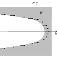
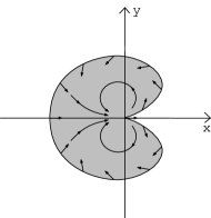
Definition 2.2
Let be such that , where . An attracting petal for centered at an attracting direction is a simply connected open set such that
-
a)
-
b)
-
c)
with for all
A repelling petal centered at a repelling direction is an attracting petal for centered at the attracting direction for .
We should note that an attracting (resp. repelling) direction is an element of such that (resp. ). Moreover, the union of the attracting petals and the repelling ones constitutes a neighborhood of the origin.
In the case that we have exactly one attracting petal (resp. direction) and one repelling petal (resp. direction). The general case where can be treated in a similar way. In fact, this case can be reduced to previous one. Let . Up to conjugation by an homothety, we can suppose that . Now conjugating by we obtain
Thus we are reduced to the case , which has been analyzed before. We note that the sectors are mapped conformally, by , onto the plane minus the negative real axis. This implies that in the case we have essentially a ramification of order of the previous case. The mapping has therefore attracting petals . The petals are (invariant domains) bounded by piecewise analytic Jordan curves () and they are symmetric relatively to the rays . At the origin, has two tangents . The final picture is summarized by the theorem below.
Theorem 2.5 (Flower Theorem)
Let be given by , where . Denote by the attracting directions and by the repelling ones. Assume that they are ordered by the following rule: starting at and moving in the counterclockwise direction we first meet and then . Then
-
a)
For each (resp. ) there exists an attracting (resp. repelling) petal (resp. ) centered at (resp. )
-
b)
The union of all attracting and repelling petals constitutes a neighborhood of the origin
-
c)
and for
-
d)
The diffeomorphism is holomorphically conjugated to the translation map on each attracting petal.
We recall that a domain is called a Leau domain if is conjugate to the translation on and also if the sequence converges to a point on . The cardioid-shaped region illustrated on Figure 2.2 is an example of a Leau domain.
2.2.3 Some Normal Forms in Higher Dimensions
The Cauchy Majorant Method was essential to prove the convergence of the formal conjugating diffeomorphisms for generic vector fields in dimension . We begin this section noticing that the generalization of this result to higher dimension is straightforward. We will not prove it.
Theorem 2.6 (Cauchy Majorant Method in Several Variables)
Let , , be holomorphic functions with trivial linear part and let , , be formal series. Consider the change of coordinates
| (2.17) |
and assume the existence of such that
for all . Then the series of converges and hence defines a holomorphic change of coordinates.
We shall obtain the correspondent to Theorem 2.3 for several variables. Before that let us introduce some definitions.
Definition 2.3
Suppose that the origin is a singular point of a vector field on . Let be the vector of eigenvalues of . We say that the eigenvalues are resonant if, for some , there exists with such that
i.e. if at least one of the eigenvalues can be written as a non-trivial positive linear combination of all of them. In this case the monomials are said to be resonant. Like in the two dimensional case, if then is said to be -resonant.
Definition 2.4
We say that a -tuple belongs to the Poincaré’s domain if the convex hull of the complex numbers , i.e. if the set , does not contain the origin . Otherwise we say that belongs to the Siegel domain.
A linear vector field defined on is said to be of Poincaré-type (resp. Siegel-type) if its spectrum is in the Poincaré’s domain (resp. Siegel’s domain).
To belong to the Poincaré domain is equivalent to the existence of a straight line through the origin such that all the eigenvalues belong to a same half-plane defined by this straight line.
Theorem 2.7 (Poincaré Linearization Theorem)
Let be a holomorphic vector field defined in a neighborhood of the origin of such that its linear part is of Poincaré-type. Let be the eigenvalues of . Assume that there there exists no resonance relation. Then there exists a holomorphic change of coordinates that linearizes .
Proof. The idea of the proof is the same as in the case of dimension . Substituting Equations (2.17) in the differential equation associated to , we obtain the following relations
for , where and , with . Due to the non-resonant assumption, we have that for all . Thus the equations above are solvable in order to , for all and . and, consequently, is formally linearizable. In order to prove the convergent it is sufficient to prove that is bounded from below by a positive constant. The proof goes as in the two dimensional case.
Let be a positive constant such that . Therefore,
Since , we have
The convergence of the desired coordinate change results by applying Theorem 2.2.
Now we shall approach the case of a saddle-node singularity in dimension . First we will consider the case where only one of the eigenvalues is zero.
Theorem 2.8
Let be a holomorphic vector field defined in a neighborhood of the origin of . Denote by the eigenvalues of the linear part of at the origin. Assume that . Assume also that are non-vanishing eigenvalues not satisfying any resonance relation and belonging to the Poincaré domain. Then there is an analytic change of coordinates where the original system is given in terms of vector fields by
with . In particular, is an invariant 2-plane.
Proof. Using the same notation as before, we consider a formal change of coordinates such that:
As in Theorem 2.7, the assumption over the eigenvalues guarantee the existence of a positive constant such that . Hence,
Notice that depends only on and , so that the last term in the above estimate vanishes for . On the other hand, by construction, all the non-zero coefficients are associated to monomials that depend on , in such a way that we are able to conclude:
and, as before, the application of Theorem 2.2 concludes the proof.
Next, let us consider the case where two eigenvalues are equal to zero. We will notice that the method used in the previous case to prove the existence of an invariant plane does not work in the present situation.
Let be a holomorphic vector field defined in a neighborhood of the origin of , whose linear part has eigenvalues and . We could try to see if the previous method allows us to prove the existence of an invariant plane. Let be given, in local coordinates, by:
where are holomorphic functions of order at least . Using the same method it is possible to prove the existence of a formal change of coordinates such that is divisible by , and , are divisible by . In this case, the plane is invariant under . However, the method used in the above situation does not allow us to prove the convergence of the series.
Let us now go back to the saddle-node case with exactly one eigenvalue equal to zero.
Theorem 2.9
Let be a holomorphic vector field defined in a neighborhood of the origin of , with eigenvalues , and . Let be an arbitrary positive integer. Then there is an analytic change of coordinates where the original system is given in terms of vector fields by
such that , i.e, the axis is invariant under .
Proof. Consider a change of variables of the form
| (2.18) |
We have to show that can be chosen so as to fulfill our requirements. In the coordinates the vector field is given by
| (2.19) |
In the above formula, the functions admit respectively the expressions below:
| (2.20) | |||||
| (2.21) | |||||
| (2.22) |
In the above equations, the components represented as do not contain neither constants nor terms depending only on . In other words these components belong to the ideal .
On the other hand, we want to consider the terms depending only on which appear in the first coordinates of . After performing the matricial product (2.29), these coordinates are respectively given by
| (2.23) | |||
| (2.24) |
We now consider the Taylor expansions of , namely we set
| (2.25) |
Furthermore the assumption on the linear part of and the expression of the change of coordinates in (2.18) allow us to write
| ; | |||||
| (2.26) |
Because we just want to cancel the coefficients of degree less than which depend solely on , the Equations (2.23) and (2.24) can respectively be replaced by (2.27) and (2.28) without loss of generality, where
| (2.27) |
and
| (2.28) |
In view of the two formulas (2.27) and (2.28) above, the proposition is reduced to the following claim.
Claim: The coefficients are constant (that is they do not depend on ). Furthermore are polynomials on for . In addition, are polynomials on for . In particular none of these coefficients depend on .
Proof of the Claim . The facts concerning () are immediate consequences of (2.25) and of the form of the change of coordinates (2.18).
The assertion regarding () has a similar justificative which however deserves further comments.
When we perform the change of coordinates given by (2.18) and consider, for instance, , we obtain
for appropriate holomorphic functions . Moreover represents terms which do not depend solely on the variable while represents terms which are neither constant nor depend solely on the variable . Fix a monomial of having degree . The coefficients entering into the term are those corresponding to the monomials such that . This implies the claim. The proof of the theorem is over.
2.3 Advanced Aspects of Singularities
2.3.1 Saddle-Node in Dimension
Basic Properties
As was seen earlier, for a foliation (or vector field) with a saddle-node singularity in there is a holomorphic change of coordinates, by means of which may be given by the -form (the Dulac’s normal form):
where , and the order of at with respect to is at least .
Let us consider the formal change of coordinates:
| (2.29) |
taking into its formal normal form , where and
A careful look shows that the functions are holomorphic on a common neighborhood of , though the change of variables is not necessarily convergent. In other words, the -forms, and are not holomorphically conjugate, in general.
Example 2.1
Let us consider the following example due to Euler:
It admits a formal solution given by
which does not converge in any neighborhood of . Therefore the vector field cannot be holomorphically conjugated to its formal normal form.
In this section we are going to discuss the problem of the analytic classification of saddle-nodes following [Ma-R]. Our purpose is to summarize the main points of [Ma-R] by explaining the role of the sectorial normalizations along with the analytic invariants of the diffeomorphisms arising from “changing the sector”. By a sector with vertex at , we mean an angular sector of angle , intersected with the ball of radius centered in .
Let be a holomorphic function in , where is a neighborhood of and is a sector with vertex at . We say that is the asymptotic expansion of at if for each there exists such that for every :
The idea is that certain formal series can be realized as asymptotic expansions of holomorphic functions that are defined on sectors of angles and sufficiently small radius . In other words they are not defined on a neighborhood of zero, otherwise the series would have to converge since they would agree with the Taylor series of the functions.
The next theorem, due to H. Hukuara, T. Kimura and T. Matuda [H-K-M] implies that, although in general the -forms and are not holomorphically conjugate in neighborhoods of , they are actually holomorphically conjugate in conveniently chosen sectors.
Theorem 2.10 (Hukuara-Kimura-Matuda [H-K-M])
Let be a formal series as defined in (2.29), i.e. the change of coordinates that takes into . Then, for every sector of angle less than , there exists a bounded holomorphic map
such that:
-
1.
;
-
2.
is the asymptotic expansion of at .
is called a normalizing application.
To simplify, we will consider the particular case of . Note that the cases may be dealt with in a similar way, except that the number of sectors which are necessary to cover the ball centered in increases. The general procedure would be a straightforward generalization of the case somehow in the spirit of the Flower Theorem (2.5) compared to the case (cardioid-shaped region).
According to Hukuara-Kimura-Matuda Theorem, we can cover the neighborhood of with two sectors of angles less than . To fix ideas, we may suppose that and . Notice that has two connected components. The bisectrix of one of them is the positive real semi-axis, therefore we shall denote it by . Analogously for , the component whose bisectrix is the negative real semi-axis.
Let us consider the foliation induced by the equation on a neighborhood of . Let (resp. ) be the restriction of the foliation to (resp. ). Naturally and coincide in the intersection of the domains, so we denote the foliation in (resp. ) by (resp. ).
Theorem 2.10 assures the existence of normalizing applications and defined on and , respectively. In the following, our aim is to understand the behavior of the applications that are responsible for the changing of sectors. First of all, the change of sectors gives rise to two diffeomorphisms denoted by and . The first one corresponds to the restriction of to while the second one corresponds to the restriction of the same map to . The next proposition gives a characterization for these functions.
Proposition 2.1
The diffeomorphism is a translation and the diffeomorphism is tangent to the identity.
Before proving this proposition we will give a geometric approach to and . Firstly, notice that the solutions of , i.e. the leaves of the foliation, are given by
| (2.30) |
with . So each leaf of (resp. ) is in correspondence with . In other words, the leaf space is isomorphic to , being parameterized by the constants . Therefore (or , depending on whether or ) is defined on and (or ) is the corresponding leaf when we change sectors.
The following is classical after [Ma-R], we follow however the discussion in [R1]. Fix a sector and let us consider the group of automorphisms , such that each element is a diffeomorphism defined on with the following properties:
-
1.
,
-
2.
is asymptotic to the identity,
-
3.
preserves the foliation induced by , i.e. .
Note that if are normalizing applications on , respectively, then the restriction of to (resp. ) is an element of (resp. ). The normalizing application obtained in Theorem 2.10 is not however uniquely defined. Indeed, if is a normalizing application in , then so is , for all . In other words, the normalizing application is uniquely defined up to the composition with an element of . This is why the change is not the identity in general. The change is indeed an asymptotic expansion of the identity. More precisely, it is an element of . The special case in which the gluing of the leaves is the identity is exactly the case where the formal normal form is holomorphically conjugate to Dulac’s normal form.
Proof of Proposition 2.1. As already mentioned, the sector change is an element of . Indeed Theorem 2.10 guarantees that conditions and are fulfilled. As to the third condition, we notice that () are such that:
where is the given vector field (i.e. ) and is its correspondent formal normal form (i.e. ). Thus,
The map belongs to , if it is asymptotic to the identity and preserves the foliation. If we think in terms of vector fields the last condition implies that:
| (2.31) |
while the first one is satisfied if and only if the functions are asymptotic to the zero function when tends to . The left hand side of Equation 2.31 is given by
while the right one is given by
The equality between those expression leads us to the following ordinary differential equation:
whose solution is given by
where is the initial data. Therefore unless we have
for all , where by we mean the real part of . We have therefore that, for , is asymptotic to the null function if and only if or . This is equivalent to say that on for all , i.e. that takes the form
In the same way we notice that
Therefore or or in order to to be asymptotic to the null function. This implies that vanishes identically on , i.e. that is tangent to the identity.
Since each leaf of is parametrized by a constant (Equation 2.30) the diffeomorphismes can be expressed in terms of the parametrization by those constants. In this way Proposition 2.1 says that
Now given two saddle-node foliations that are holomorphically conjugate, it is interesting to work out the relation between their sector changing diffeomorphisms (which in the case, we denoted by and ). Indeed, we are going to see that if the saddle-nodes are holomorphically conjugate, then their sector changing diffeomorphisms are also conjugate by an automorphism of the leaf space. The converse is also true, though it will not be fully proved.
Let and be holomorphically conjugate foliations given by -forms and , respectively. In other words, there exists a diffeomorphism that takes the leaves of in leaves of . There are also formal changes of coordinates and that take and , respectively in formal normal forms and . As was seen in the earlier discussion, though (resp. ) is not analytic on a neighborhood of , there are sectors in which the series does converge. In the case there are functions , (resp. , ) that glue together the leaves of the sectors and .
We shall define the following equivalence relation: two diffeomorphisms and are said to be equivalent (and we write ) if there exists with such that:
In other words, conjugate functions belong to the same equivalence class. In this sense, if the foliations are holomorphically conjugate, the transition function (resp. ) is equivalent to (resp. ). Indeed, notice that the function is an automorphism of the leaf space (which is isomorphic to a neighborhood of as observed in Formula 2.30) tangent to the identity. Denoting by the restriction of to and by the restriction of to it follows that and .
Summarizing, the analytic type of saddle-nodes with are in correspondence with the conjugacy class of the diffeomorphisms and . Since the conjugacy class of translations is obvious, we can think that the information is totally encoded in the conjugacy of the diffeomorphism tangent to the identity. It is then natural to study the moduli space of diffeomorphisms of tangent to the identity so as to have concrete invariants for saddle-node singularities.
Automorphisms of with identity linear part
Now we will concentrate on the study of the automorphisms of tangent to the identity that were used in the above definition of equivalence relation. The description of the moduli spaces is independently due to Ecalle and Voronin. In what follows we shall follow Voronin construction for the prototypical case .
Precisely, we shall give an analytic classification of the mappings of the set . As usual, we define two mappings , to be equivalent if and only if there exists a holomorphic diffeomorphism such that . Here we describe these classes of equivalence.
To begin with we give some Analysis results and definitions that will be used in this section.
Definition 2.5
A homeomorphic mapping of a domain is said to be quasiconformal if
for almost everywhere.
The function is called the characteristic of the quasiconformal map , and the quantity
is called the quasiconformal deviation of the map at the point . Notice that if is a quasiconformal map with characteristic , then is conformal.
Proposition 2.2
A map is quasiconformal in if and only if for all and .
Theorem 2.11 (Measurable Riemann Theorem)
For any measurable function such that , there exists a quasiconformal map of the plane onto itself, having the function as its characteristic .
Next, we consider the specific case of the function in . Notice that the inversion conjugates conformally to the translation on , that is,
| (2.32) |
Next we are going to see that the last remark holds in general. Namely for every function belonging to , there always exist certain domains in where is quasiconformally conjugate to . We prove this by using the next two results.
Theorem 2.12 (A. Shcherbakov)
Let , . For every one can find and a homeomorphism of the disk (of radius ) onto itself such that:
| (2.33) | |||||
| (2.34) |
This theorem basically asserts that every function tangent to the identity is, in a sufficiently small disk, conjugate to by a Lipschitz mapping with Lipschitz constant close to . The proof of the theorem amounts to some finer estimates involving the Fatou coordinates [Car-G].
Lemma 2.5
Suppose that for the homeomorphism , Estimate (2.34) holds for , then is quasiconformal in .
Proof. This lemma follows immediately from Proposition 2.2. Indeed, under these conditions, the quasiconformal deviation of , is such that for .
Proposition 2.3
For each there exist domains and a quasiconformal mapping defined on , satisfying
-
•
on ,
-
•
on .
Proof. Fix such that . From Theorem 2.12 there exists a homeomorphism , conjugating and as in (2.33). Moreover, this homeomorphism is quasiconformal by Lemma 2.5.
Let for a fixed complex number with . The mapping defined on is well-defined and quasiconformal, being a composition of a quasiconformal map with a conformal one. Set . It follows from (2.32) and (2.33) that is precisely the conjugacy we were looking for. In conclusion, is quasiconformally conjugate to a translation.
Moreover, since it follows that is invariant by , i.e. . Analogously, we can define a domain that is invariant by . More precisely, where with as before. Naturally, is defined on and is quasiconformally conjugate to the translation . Thus establishing the proposition.
Equivalently, one may define the domains and so as to make their boundaries smooth (refer to [Car-G]). Under these circumstances is the well-known cardioid-shaped region (cf. Section ). The reader may keep this figure in mind whenever we refer to and as it may help intuitively.
The next lemma gives analytic coordinates and defined on the domains and . In what follows, we can trace a parallel between the saddle-node case, analyzed in the previous section, and the gluing of the domains and . In this sense, we are still considering conjugacies which are not defined on a full neighborhood of the origin. In the saddle-node case, we have sectorial normalizations that are provided by Hukuara-Kimura-Matuda Theorem. The analogue of this theorem in the present case is the lemma below.
Lemma 2.6 (Basic Lemma)
Let and be as before. Set and consider a quasiconformal homeomorphism of the domain onto . Let be analytic in such that
| (2.35) |
Then there exists an analytic mapping satisfying
-
1.
is univalent in .
-
2.
.
-
3.
If is another analytic mapping on verifying conditions and , then there exists such that on .
Notice that an analogous lemma may be formulated for the existence of the analytic mapping with the obvious modifications.
Proof. As already seen, is conjugated to a translation. What this lemma asserts is that the conjugating homeomorphism is, in fact, analytic.
The quotient space is conformally equivalent to the punctured plane , where is the projection. Since is a homeomorphic mapping satisfying (2.35) the orbits of are discrete and is a Riemann Surface. Let be the projection of the quotient space. From (2.35), we obtain a quasiconformal homeomorphism between the quotient spaces.
Claim : If there exists a conformal mapping then there is an analytic mapping verifying , and .
Indeed, notice that is a covering for with holomorphic projection . However, the universal covering of is with projection . Since is a simply connected covering of then there exists an inclusion such that . This mapping satisfies , and (details may be found in [Vo]).
Claim : If there exists a quasiconformal mapping , then is conformally equivalent to .
Since is a quasiconformal mapping from to a domain , the characteristic of its inverse is independent on the choice of a local parameter on , and . Setting , remains measurable and . By Theorem 2.11 there exists a quasiconformal homeomorphism of onto itself with characteristic and we may suppose that . So that the map is conformal.
Now we analyze the functions that change the sector, i.e. the analogous to the functions in the saddle-node case.
Let (resp. ) be the restriction of (resp. ), where and ( denotes the imaginary part of ).
Remark 2.1
It is not obvious, but with some effort an expression for may be obtained. More precisely, (cf. [Vo]).
To each we may associate a pair of holomorphic functions. Since we are interested in the classes of conjugacy of the elements of , it is natural to work out the relations between the maps and associated to conjugate diffeomorphisms and , respectively. The advantage of the preceding construction lies in the fact that the corresponding transition maps are related in a particularly simple way. Indeed, by Lemma 2.6 there exists analytic mappings and such that:
By assumption, so that
Suppose that is given by Lemma 2.6 for . Then by item of this same lemma, it follows that
Similarly,
where and are translations. Then
In conclusion, we have obtained the following
Theorem 2.13
If and belong to the same class of analytic equivalence then the transition functions and are conjugate by a translation.
Remark 2.2
The reader may notice that, starting from the problem of classifying the saddle-nodes, we have iterated twice a procedure of “sectorial normalization”. This might give the impression that no real progress was made in the second iteration towards a concrete description of a suitable moduli space. This is however not the case. In fact, in the saddle-node case, we have used sectorial normalizations provided by the Hukuara-Kimura Matuda Theorem to obtain diffeomorphisms , where conjugacy classes determine the analytic type of the saddle-node. The difficulty is that is tangent to the identity but it is not uniquely determined. Only the conjugacy class of in is canonical in the sense that it is uniquely determined. Thus, in a “concrete” comparison between two saddle-nodes we would be reduced to tell whether or not two “different” diffeomorphisms tangent to the identity are conjugate in . The answer to this problem is by no means obvious. To tackle this new question, we again applied sectorial normalizations (this time provided by the Basic Lemma) to obtain new functions . The advantage of this second normalization is that are “almost uniquely determined”, in the sense that two of them are conjugate by a translation. In particular, it is easy to decide whether or not two of them define the same point in the corresponding moduli space.
2.3.2 Reduction of Singularities in Dimension
So far we have only been analyzing vector fields with simple singularities. However, as it will become clear throughout this section, there is a particularly effective way of dealing with higher order singularities. The Seidenberg Theorem basically asserts that by composing a finite number of blow-up applications, it is possible to reduce the order of an isolated singularity until we only obtain simple ones. This section is devoted to explain how it can be done.
The reader will notice that the present exposition is very strongly inspired in the treatment given in [M-M], which, in turn, is a blend between the original work of A. Seidenberg [Sd] and that of Ven den Essen.
Let us now fix notations and give a few definitions. Suppose that is a singular holomorphic foliation associated to the holomorphic vector field having an isolated singularity at . We can also think in terms of -forms. After all, the -form and the vector field define the same foliation . The eigenvalues of at are defined to be the eigenvalues , of at the same point.
Let (resp. ) denote the homogeneous component of degree of the Taylor series of (resp. ) centered at the origin. Let be the degree of the first non-trivial homogeneous component of the -form . The blow-up of in the coordinates is given by:
while in the coordinates it is given by:
where
We adopt an analogous notation for .
Let , and denote by the subset of the exceptional divisor formed by the singularities of the “new” foliation (i.e. the foliation associated to ). Notice that in the non-dicritical case ( is not identically zero) the set is given by the solutions of . Denote by the order of the singularity .
Suppose that is a mapping defined on with a singularity at . The order of at , denoted by , is the degree of the first non-trivial homogeneous component of the Taylor series of based at the origin. We may also define the order of a vector field (as was done in Section ). If is singular at the order of is the minimum between the orders of and . Analogously one may define the order of a -form at .
Let be two polynomials defined on . Consider two algebraic curves and associated, respectively, to and , i.e. consider
and suppose that they intersect each other at . Recall that if is irreducible then there exists a local normalization (Puiseux Parametrization)
for a certain and . We are now able to introduce the notion of intersection number of two algebraic curves.
Definition 2.6
If is irreducible then the intersection number of and at is defined to be
If is not irreducible but , where are irreducible, then the intersection number of and at is defined to be
Finally, the intersection number of the -form is defined to be
At this point we are able to state Seidenberg’s Theorem.
Theorem 2.14 (Seidenberg)
Let be a singular holomorphic foliation associated to the -form defined on an open set admitting an isolated singularity at . There exists a proper analytic application obtained as a composition of blow-ups of a complex -dimensional manifold onto , such that:
-
•
, where is the exceptional divisor of ;
-
•
is a holomorphic diffeomorphism;
-
•
for all
In other words, the proper transform of is defined on a complex manifold and is such that all of its points are either regular or simple singularities.
Proof. Suppose that is the only singularity of in . Let be the order of at . If , we use the blow-up procedure, described in Section . In other words, we consider the pull-back of by the proper mapping given by . Let denote the exceptional divisor. In coordinates the blow-up of is given by
| (2.36) |
with as above.
As previously seen, the behavior of varies significantly on the neighborhood of depending on whether or not is identically zero. By analyzing these two different cases, it is not hard to obtain equalities relating the intersection number of and its order at (refer to [M-M] for details). More specifically,
-
•
If is not identically zero, i.e. if the exceptional divisor is invariant under the foliation, then
(2.37) -
•
If , then
(2.38) This corresponds to the dicritical case, i.e. to the case where the leaves of the foliation associated to are regular and generically transverse to .
There are two possibilities, either the -form has only simple singularities and regular points on and the theorem is proved, or there still are points , such that . So, let us assume that the second case occurs. We first set
Next, we simultaneously blow-up all the points such that . Let be the resulting application corresponding to these blow-ups. We then define
Inductively we construct applications , by blowing-up all the points of such that , where
The Equations (2.37) and (2.38) guarantee that this procedure is finite. Indeed, despite the two different behaviors the blown-up foliation may assume, in both cases the intersection number decreases if . So if we repeat this procedure sufficiently many times, there will be a large enough such that for every on , .
Now we shall treat the case of a foliation with only simple singularities. By performing additional blow-ups it is possible to obtain a simpler expression for the -form associated to . This corresponding form cannot be further simplified by extra blow-ups, and in this sense they are “final” or “irreducible”.
Theorem 2.15
Consider the singular holomorphic foliation associated to the -form defined on with an isolated singularity at . Let the blow-up application obtained by Theorem 2.14. Then for every where , there exists a coordinate chart centered on such that
| (2.39) |
where , and , do not belong to , or
| (2.40) |
Let us begin our approach to Theorem 2.15 by stating the following result:
Lemma 2.7
Suppose that the -form is non-dicritical. If there exists such that , then . In other words, the blow-up of at , , does not raise the order . Moreover, has a non-zero eigenvalue.
Proof. We may suppose that the order of at is . According to the eigenvalues of , there are different situations that should be analyzed separately:
-
1.
;
-
2.
;
-
3.
, and , belong to ;
-
4.
, and , do not belong to ;
-
5.
, .
Notice that the cases and correspond precisely to the situations reflected by Equations (2.39) and (2.40), respectively. Now we show that by blowing up the manifold on certain points, the previous cases are reduced to cases or .
Case
In this situation, the jacobian matrix
of the vector field at is similar to
Therefore, , so that the set is formed by the point and .
Now we blow-up the foliation at , obtaining
Suppose that .
Notice that the order of may be or depending on whether or not is equal to zero. We analyze the two possibilities separately:
-
•
(1.a)
In this case, and to simplify the notation we denote by:
Notice that is given by the equation
hence formed by the point with . Now we blow-up at and in the coordinate chart , to obtain
Therefore, is given by the equation
and hence it contains only simple points. By applying Lemma 2.7, we conclude that in these coordinates . Therefore we have reduced to a -form which does not belong to Case .
-
•
(1.b)
Here, , and as before, denote by . The set is given by
for certain constants , , and .
-
–
If we apply Lemma 2.7 and the conclusion is the same as before.
-
–
If then
Hence the jacobian matrix associated to is , therefore admitting a non-zero eigenvalue.
-
–
If then the point , has multiplicity and
So, is still of the same type as . Notice that by Theorem 2.14 . Therefore this possibility leads to Case (1.a).
-
–
In conclusion, there always exists a way to blow-up so that both of its eigenvalues are different from zero.
Case
Without loss of generality we may suppose that . Hence there are basically two possibilities to be considered:
-
•
The jacobian matrix of the vector field at is similar to
In this situation, . It is therefore the dicritical case. By blowing-up at each , notice that has no singularities ( for all ).
-
•
The jacobian matrix of the vector field at is similar to
Here, , and the set is the point with . By blowing-up at we obtain:
Notice that the jacobian matrix associated to at is equivalent to . This corresponds to Case , so that is reduced to Equation (2.40).
Case
In this case, . We may suppose that and . So, may be written as
Notice that there are exactly two points on , namely and . Blowing-up at on the coordinate chart , we obtain
so that the jacobian matrix is:
Therefore, we have reduced to a -form having eigenvalues and there are three possibilities for :
-
•
If then and the reduction of belongs to Case .
-
•
If then and the reduction of belongs to Case .
-
•
If then and by blowing-up times, the reduction of belongs to Case .
Now let us analyze the blowing-up of at on the coordinate chart , where
Hence the jacobian matrix is given by:
-
•
If then and , hence the reduction of belongs to Case .
-
•
If then and , hence the reduction of belongs to Case .
-
•
If then and , hence the reduction of belongs to Case .
This completes the proof of the theorem.
2.3.3 Existence of First Integrals
To illustrate the applications of the preceding techniques on concrete problems about singularities of foliations, we shall provide in this section a detailed proof of a fundamental result due to J.-F Mattei and R. Moussu [M-M] concerning the existence of first integral for those singularities.
Recall that a holomorphic first integral of a holomorphic foliation is a non-constant holomorphic function that is constant when restricted to the leaves of . If is a -form defining then is such that . Equivalently, the leaves of are the irreducible components of the level surfaces of .
This section is devoted to the topological characterization of foliations admitting a holomorphic first integral, which is itself the main result of [M-M].
Let be a holomorphic foliation defined on an open set , with an isolated singularity at . Suppose that is a holomorphic first integral for . Then the following conditions hold:
-
1.
Only a finite number of leaves of accumulates on .
-
2.
The leaves of are closed as subsets of .
Indeed, if this function exists then the set is the set of the separatrizes of . Recall that a separatrix is simply an irreducible analytic curve invariant by , which contains the singularity. Now can have only finitely many irreducible factors, i.e. for some positive integer constants and holomorphic functions such that . Hence the number of separatrizes must also be finite, as these are given by the equations . Clearly this is the contents of Condition .
Since is constant when restricted to the leaves, Condition also holds. In particular, a leaf of that is not contained in the set cannot accumulate on a separatrix. This last remark will often be used in the sequel.
Conversely, a foliation satisfying Conditions and admits a first integral. This is the contents of the next theorem that plays the main role in this section.
Theorem 2.16 (Mattei-Moussu [M-M])
Consider the holomorphic foliation defined on an open set with an isolated singularity at . Suppose that it satisfies the following conditions:
-
1.
Only a finite number of leaves of accumulates on ;
-
2.
The leaves of are closed on .
Then has a holomorphic non-constant first integral .
Before proving the theorem, consider two holomorphic foliations with isolated singularities, and defined on a neighborhood of the origin. We say that and are topologically equivalent if there exists a homeomorphism , such that taking the leaves of into the leaves of . It follows from the above theorem that the existence of a holomorphic first integral obeys a topological criterion: if admits one such first integral so does .
Roughly speaking, the proof of Theorem 2.16 consists of three main steps. These are as follows:
Part : If satisfies Conditions and , then, by performing successive blow-ups, the only irreducible singularities found in the Seidenberg tree are those having two non-zero eigenvalues and verifying in addition . Thus the singularities belong to the Siegel domain.
Part : Study of on a neighborhood of a singularity in the Siegel domain. In particular the characterization of those possessing a holomorphic first integral.
Part : Extension of the local “first integrals” obtained in Part to a neighborhood of the exceptional divisor . If denotes this extension, then is the first integral we were looking for.
We will give a detailed approach to each part described above in the next sections. Together, they will conclude the proof of the Mattei-Moussu Theorem.
Part : Analysis of Singularities in the Seidenberg Tree of
Let us now begin by analyzing the irreducible singularities obtained by the Seidenberg procedure. From now on we shall assume that satisfies the assumptions of Theorem 2.16.
Proposition 2.4
Let be a foliation satisfying Conditions and . Then the only irreducible singularities that exist in the Seidenberg tree of are those having non-zero eigenvalues and such that the quotient belongs to .
As seen in the previous section, every singularity of a given foliation may be reduced by successive blow-ups so that the blown-up foliation only contains simple singularities with eigenvalues and which fall in one of the following cases:
-
•
where at least one between is distinct from zero (the case of a saddle-node singularity).
-
•
with neither nor being a positive integer.
Let us discuss the different possibilities separately.
Lemma 2.8
The Seidenberg tree contains no saddle-nodes.
Proof. Suppose for a contradiction that the statement is false. As we have seen in previous sections there are local coordinates about a saddle-node singularity where the blown-up foliation is given by
Note that is invariant by the blown-up foliation . Next let us consider the holonomy application of associated to a small loop contained in encircling the origin. We have already seen on Section 2.2.2 that the holonomy is given by for on some local transverse section .
From the dynamical structure of (in particular the existence of Fatou coordinates) we see that there are infinitely many points whose orbit under the iteration of accumulats on . These points naturally correspond to distinct leaves of accumulating on the regular part of . Now we have two possibilities.
If is contained on the exceptional divisor, then it is projected onto . Hence there are infinitely many leaves accumulating on the origin. This is not possible, for we are assuming Condition .
On the other hand, if is transverse to the exceptional divisor, then it is projected by as a separatrix (recall that is proper). There are infinitely many leaves accumulating on this separatrix, which again is impossible, since it contradicts Condition .
In conclusion the reduction of does not contain any saddle-node singularity.
Next we shall discuss irreducible singularities having two eigenvalues , different from zero. Recall that such a singularity is called hyperbolic if .
Lemma 2.9
There is no hyperbolic singularity in the Seidenberg tree.
Proof. By the Poincaré Linearization Theorem (cf. Section 2.2.1) we may suppose that the vector field associated to is given in local coordinates by
Again, is invariant by the foliation and, in order to study the behavior of the leaves close to , we are going to consider its local holonomy.
Let be a small loop around the origin of . Let be a transversal section to the leaf through the point . The lift of the loop to the leaf through the point is described by the differential equation
whose solution is given by . Hence the holonomy map turns out to be . However we have that since is not in . Now by iterating , we obtain
where and . The absolute value of is determined by the value of . More specifically, if then tends to zero as increases and, consequently the correspondent leaf accumulate on . If then goes to zero as goes to minus infinity. This also ensures that our leaf accumulate on . However, Conditions and prevent this type of behavior from happening and we conclude that the reduced foliation does not contain this kind of singularities.
Lemma 2.10
The Seidenberg tree does not contain singularities with non-zero eigenvalues such that .
Proof. By Theorems 2.3 and 2.15, the vector field is still linearizable and is invariant by the correspondent foliation. Notice that in this case the holonomy application will not help us to conclude that this singularity does not occur. In fact the holonomy map has the form for some , i.e. the holonomy is conjugate to a rotation of .
However, by following the radial lines connecting a point on the plane to the origin, we see that the neighboring leaves accumulate on the origin. Indeed, fix a point and consider the lift of the radial line , , contained in to the leaf through . This lift is described by the differential equation
whose solution is given by . Since the quotient is positive it follows that goes to as goes to infinity. Ultimately, this implies that there are infinitely many leaves accumulating on . Again, such singularities do not appear on the blown-up foliation.
Finally, we have reached the conclusion that we may assume that the blown-up foliation only has singularities with eigenvalues such that . Before proceeding we only remark that:
Lemma 2.11
All the irreducible components of the Seidenberg tree are invariant by the corresponding foliation.
Proof. If it were not so there would be infinitely many separatrizes, contradicting our assumptions.
Remark 2.3
The argument used in the preceding lemma can be extended to show that a singularity has infinitely many separatrizes if and only if by performing a finite sequence of blow-ups, we arrive to an irreducible component of the total exceptional divisor which is not invariant by the corresponding foliation. This type of singularity is called dicritical.
The above lemmata leading to Proposition 2.4, corresponds to the first part of our proof.
Part : Existence of Local First Integrals
Let us take a closer look at the only singularities that appear in the Seidenberg tree, i.e. those having eigenvalues such that is in . We obtain from Lemma 2.2 that in local coordinates , the vector field is given by:
| (2.41) |
for . First, what needs to be studied is whether or not this vector field is linearizable. More generally we would like to tell when two vector fields as above (with , fixed) are conjugate. The next proposition due to J.-F. Mattei and R. Moussu is of fundamental importance for it allows us to restrict ourselves to understanding whether or not the corresponding holonomy is linearizable (conjugate).
Theorem 2.17 (Mattei-Moussu [M-M], [M])
Assume that are given in coordinates by Equation (2.41) with . Denote by (resp. ) the holonomy of (resp. ) relative to the axis . Then there is an analytic diffeomorphism defined on a neighborhood of and conjugating if and only if there is an analytic diffeomorphism defined on a neighborhood of and conjugating .
There are two markedly different cases to be considered according to whether or not is rational. Firstly, suppose that where . In this case, the holonomy of associated to a loop around the origin in the separatrix , is given by
where is the parameter on a local section transverse to . This application is linearizable if and only if . It is obvious that if is linearizable then . The converse is not obvious but can easily be verified by noticing that linearizes . Note that when it is not linearizable (i.e. when ) we end up in the case already studied. Namely, we end up on the dynamics of the cardioid-shaped region analyzed on Section 2.2.2. Similarly to the saddle-node case, this cannot occur since otherwise we would have infinitely many leaves accumulating on , what contradicts our assumptions.
Hence, we may suppose that is indeed linearizable. From Theorem 2.17, the vector field associated to admits the normal form, given in local coordinates by
| (2.42) |
Let us now focus on the case where is irrational. As before, the holonomy application is given by . However, since is an irrational number, the difficulty of knowing whether or not is linearizable increases considerably. The problem of finding out which are the irrational values of that make the holonomy linearizable is known as the “Siegel Problem”. In fact, for certain values of , it is possible to obtain local diffeomorphisms as above that are non-linearizable.
Remark 2.4
Note that it is not difficult to obtain a formal conjugacy that linearizes any such . More precisely, by formally solving , one obtains , with and
To deal with the irrational values of , let us first consider the linearizable case. Then is conjugate to an irrational rotation of . Let be the set formed by the points of intersection between the leaf of passing by and the circle . As always, is the transverse section to passing by . Since an irrational rotation has dense orbits, it follows that is dense over the circle . In other words, the leaves are not locally closed, which contradicts Condition . In particular, any possible holomorphic first integral , would be constant everywhere. Indeed, the restriction of to is constant over circles about . As a result would be constant everywhere.
We are then reduced to discuss the case in which is not linearizable. To deal with this case we are going to show the existence of leaves of that are not closed on arbitrarily small neighborhoods of .
Let us begin with a simple lemma attributed to J. Lewowicz but, before stating it, we give some definitions that will be useful throughout the text. Let be a neighborhood of , where is defined, holomorphic, and injective. Let be a subset of and fix a point .
Definition 2.7
The -orbit of is the set of points on , obtained by iterating forward (i.e., , times) and backwards (i.e., , times), along with itself (denoting by ). In other words,
The number of iterations of is the number of times is iterated taking to a point on . It is denoted by and belongs to .
Note that there may exist points on such that but . These points are called periodic on . Naturally, if is finite then is necessarily finite.
Definition 2.8
An element is said to have finite orbits if there exists an arbitrarily small open neighborhood of where is defined, holomorphic, injective and satisfies
for every .
Lemma 2.12
Let be a compact connected neighborhood of and a homeomorphism of onto , verifying . Then there exists a point on the boundary of such that the number of iterations in is infinite, i.e. such that .
Proof. Denote by the interior of and let (resp. ) denote the number of iterations of on (resp. ). Suppose, by contradiction, that only attains finite values on the boundary of . Since is compact, is uniformly bounded on , i.e. there exists such that
Consider the sets
which are non-empty open sets. In fact we can verify that and . Moreover, since for all , those sets are disjoint. Notice that there exists such that does not belong to . Indeed, if it did not exist, then every would be such that , in other words, . The connectivity of would imply that or , which is impossible. Thus there exists such that . It follows that the orbit sets of on and on are different (). In other words, the orbit of passes by . Let , therefore, , contradicting .
Lewowicz’s Lemma (Lemma 2.12) ensures the existence of points whose orbit never leaves the neighborhood of . However, it does not exclude the possibility that all these points are periodic. In this direction, the next proposition will be fundamental.
Proposition 2.5
If is not periodic then there exists open neighborhoods of on such that is holomorphic, injective and for each , the set of points with infinite -orbit is uncountable and is an accumulation point.
The basic idea behind its proof is to consider sets , for such that . If the domain of were connected and then each would be a finite set. In particular, would be countable. By the lemma the set of points with infinite number of iterations is uncountable, hence there would be an uncountable set of points with infinite orbit. The difficulty with this argument is that the domain of may be disconnected and may coincide with the identity on one connected component and not on the component containing . This is why the proof of this proposition is slightly more subtle as we need to consider the various connected components of the domain of .
Proof of Proposition 2.5. Let be a closed disc centered at with radius . Using the same notations as in Lemma 2.12, we define the following sets:
Naturally, . Furthermore, Lemma 2.12 implies that for every
Claim: One of the sets, either or (or both) is uncountable.
Indeed by Lemma 2.12, for every compact disc with there is a point on its boundary with an infinite number of iterations. Hence there are uncountably many points in such that . These points belong to , thus either or must be uncountable.
Under these notations, the contents of the proposition is that the set is uncountable. Thus, it suffices to show that if is uncountable then is necessarily uncountable as well. This is what we shall do in the sequel.
Before continuing, let us define the following sets containing :
Note that is precisely the domain of definition of .
Let be the connected (compact) component of that contains and let
is, in particular, connected.
Lemma 2.13
We can assume, without loss of generality, that is countable.
Proof. Consider the case where is uncountable. Suppose for a contradiction that is countable (and uncountable). Then would also be countable. We consider now and note that it must be uncountable, otherwise would be countable, since . Let
where is the set of points of period .
Note that there exists a certain such that is infinite, otherwise all of the would be finite and would be countable. Being infinite, has a non-trivial accumulation point in . The application is holomorphic on an open neighborhood of and it is the identity on . Since this set has an accumulation point on then on , by the Identity Theorem. By construction, contains the origin so that is a neighborhood of . This contradicts the hypothesis of non-periodicity of . Hence is uncountable.
In view of the preceding lemma, in the sequel we always assume that consists of countably many points. First, note that there exists such that , otherwise would contain a point on the boundary of for every . This is obviously impossible since countable. From now on let us fix one such . We note that, in particular, .
Next, notice that the sets , for as above, form a decreasing sequence of compact sets. Hence the intersection is nonempty, unless there exists such that . The last case must occur, since was chosen so that .
Let be a compact connected neighborhood of that does not intersect the other connected components of , if they exist. In particular one has .
Lemma 2.14
For every there exists such that is not on . Besides .
Proof. To verify the existence of , suppose for a contradiction that for every , belongs to , for . In this case, would have at least positive iterations of . This means that , what contradicts the construction of .
Moreover, if there existed a periodic point of on , then would belong to every set . In particular it would belong to , what is a contradiction.
Before continuing to prove that is uncountable, we define the following sets:
Let
where is the set of the periodic points on with period .
Lemma 2.15
, where is open without boundary and is finite, consisting of isolated points.
Proof. Let be the limit of a sequence of points in . Note that we do not assume that this sequence is constituted by pairwise distinct points so that every point belonging to automatically satisfies this condition. Clearly, it suffices to show that there is a neighborhood of contained in in the case that the sequence is not trivial, i.e. is an accumulation point of the sequence. By definition, there exists an open connected neighborhood of where is defined and holomorphic. Moreover is the identity on . Hence, if is an accumulation point of the limit sequence of points in then it on from the Identity Theorem. On the other hand, the -orbit of does not intersect (cf. Lemma 2.14). Thus can be chosen sufficiently small so that . This proves that . Hence consists on the union of isolated points with . Clearly the number of isolated points must be finite, hence implying the lemma.
Lemma 2.16
The boundary of is countable consisting of the union of the isolated points in , for .
Proof. Let us first consider . Naturally it is an open set and we will prove that its boundary is empty. Suppose, for a contradiction, that there exists in the boundary of . Then there is a sequence of points in converging to . Fix a small disc about and choose a point belonging to this ball. Hence there is such that . Clearly belongs to since . Furthermore, belongs to as well since is closed. Finally, because is connected (by construction), there is a path joining to (i.e. such that , ). Since lies in and does not, there is such that belongs to the boundary of . This is a contradiction to the previous lemma. Thus is countable as the union of the finite sets .
Finally, we have one last simple lemma that will allow us to conclude the proof.
Lemma 2.17
is an open set of .
Proof. Note that, by definition, for points we have . Let
where is the set of points in such that . We claim that are open sets. Indeed by continuity of , every point of has a neighborhood of points also having iterations on . Since is the union of open sets, it is itself an open set.
To conclude the proposition we proceed as follows. Clearly we have
We shall analyze separately the following possibilities:
-
•
Suppose that .
-
•
Suppose that and .
In this case, we have that . Note that for sufficiently small values of , the compact disks are contained in . And so, by Lewowicz’s Lemma (Lemma 2.12), we have that is non-empty. Therefore, is uncountable, and as before, must be uncountable as well.
-
•
Suppose that and .
Note that and are non-empty disjoint open sets of . Thus is non-empty so it must be uncountable. Naturally, it is contained on and so, must also be uncountable.
This completes the proof of Proposition 2.5.
Proposition 2.6
Suppose that the holonomy associated to and to a local transverse section is given by , where is irrational. Then there exist leaves of that are not closed on arbitrarily small neighborhoods of .
Proof. It follows from the preceding proposition that there exists a sequence of points , pairwise distinct and accumulating on a point . In fact there exists an uncountable number of such sequences. Note that each belongs to a same leaf . We will show that the leaf passing through is not closed.
Suppose that the accumulation point is in , otherwise the claim is obvious. Suppose that there exists an isolated point of . Consider a path on connecting these two points, by continuity of the holonomy application, there is also a sequence of points of accumulating on . In other words, has no isolated points. Therefore, the closure of is uncountable (being a perfect set). However, is countable, for every leaf in a foliation can intersect a transverse section only countably many times. Hence, has points of accumulation that do not belong to it. In particular, is not closed.
Proposition 2.7
Let be a foliation satisfying Conditions and . Then its Seidenberg tree only contains singularities that admit a local first integral. In particular, the local holonomy of their separatrizes is finite.
Proof. Indeed, the preceding discussion allows us to conclude that the only possibility which does not contradict the hypothesis is when is a rational number. It follows from Theorem 2.17 that the vector field associated to is holomorphically conjugate to a linear one, locally given by Equation (2.42). Notice that its solution is given by . Hence there exists a local first integral. More precisely, is constant over the orbits of the vector field.
Now we go back to Theorem 2.17 and give an idea of the basic principles behind its proof.
Proof of Theorem 2.17. Suppose that there exists a holomorphic diffeomorphism conjugating the holonomies and relative to the foliations and , respectively and to a loop encircling the origin of a separatrix. Let be a disk of radius on a local section transverse to the separatrix (which we can assume to be given, in local coordinates, by ) at the point , whose image under is still contained in the previously chosen neighborhood.
Recall that the vector field , associated to the blown-up foliation is given by:
Note that away from , the leaves of the foliation are transverse to the vertical complex lines, i.e. to the fibers of .
First, we define a holomorphic application on the solid torus . This is done by lifting, with respect to the path along that connects to , to a path on the leaf of that passes by . Note that this lift is well-defined since the leaves are transverse to the fibers of . We also lift, with respect to , to a path on the leaf of passing by . Now we extend the diffeomorphism by declaring that takes the final extremity of to the final extremity of . We have to show that this extension of is well-defined when becomes a loop around . This is however clear, since the final extremity of (resp. ) is, by construction the image of by (resp. ) and we have . Thus we conclude that is well-defined on . is moreover an extension of , i.e. .
Next we wish to extend holomorphically to a neighborhood of and so that it still conjugates the foliations. Consider them the radial lines connecting each point on to the origin. Let be the leaf of passing by and let be the path over such that . Analogously, let be the leaf of that passes by and let be the path over that projects on by . We define to be the application that takes into by preserving the projection . By construction, is a holomorphic conjugation between and on its domain. Note that the domain of is precisely the saturated of by which is going to be denoted by .
However note that, a priori, as we follow the radial lines approaching the origin, the union of and may not contain a neighborhood of .
To be more precise, let us revisit the construction of along the radial lines . For example, consider this construction over the radial line contained in and joining the point to . By definition, we begin with a point and consider the path , , that lifts only a segment of the radial line on , going from to a point , with close to . Let be the set consisting of the final extremities, of the paths as above for every . In particular, is contained in the vertical line . The difficulty to ensure that will lead to a conjugacy defined around is related to the fact that may not contain a uniform disc about as .
In his manuscript [M], J.-F. Mattei estimates the size of the sets as above (for all the radial leaves involved and not only the example considered above of ). The fundamental result in [M] is the existence of a uniform , such that every set contains the ball of radius about . In particular, he obtains:
Proposition 2.8 (Mattei [M])
Let be a foliation with eigenvalues and , such that , then contains a neighborhood of .
The estimate of a uniform as above is done by integrating along the differential equation inducing the foliation (resp. ). It is exactly at this point that the assumptions plays its role.
This behavior is particularly clear when we consider real ODEs with real eigenvalues and satisfying . We have that increases as decreases, where . Indeed this would yield the classical picture of the phase space of a saddle (cf. Figure 2.3).
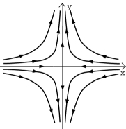
Note also that, if we consider the case , the statement would be false. Indeed, with analogous notations, the sets would be contained in balls with radii converging to zero when .
Although Mattei’s manuscript was not published, an extension to higher dimension of this result can be found in [R2] and will be treated in the next section.
Let us now go back to the proof of Theorem 2.17. Whereas is holomorphic on its domain, this domain clearly does not contain . To extend to it is however sufficient to note that is bounded by construction. On the other hand, we already know that is defined on , where is a neighborhood of . Hence the extension of to follows immediately from the Riemann Extension Theorem. Thus the proof of Theorem 2.17 is over.
This concludes the second part of the proof of the Mattei-Moussu Theorem.
Part : Extension to a Global First Integral
In this part we wish to extend the local first integrals, obtained in the previous section, to a global first integral defined on a neighborhood of the exceptional divisor of the blown-up foliation. Naturally this implies the existence of a first integral of the original foliation, hence yielding Theorem 2.16.
To explain the idea of the construction suppose first that a single blow-up application is sufficient to obtain reduced singularities on the exceptional divisor . It follows from what precedes that these singularities admit local first integrals. It will also become clear that this case already encloses the main difficulties of the general construction.
The basic idea is to extend the local first integrals around the singularities along the leaves of the blown-up foliation. If it is shown that such an extension is well-defined, then the first integral will be defined on a neighborhood of the exceptional divisor. Indeed, due to Mattei’s estimate (Proposition 2.8), the saturated of the local transverse sections by the foliation contains a neighborhood of the singularities (except for the separatrizes at each that are transverse to ). Consequently the extension would be defined on a neighborhood of , since they can again be extended over the transverse separatrizes thanks to the Riemann Extension Theorem.
To extend the mentioned first integral, it is necessary to study the projective holonomy of . Namely, note that is a regular leaf of . The holonomy associated to this leaf, which is called the projective holonomy of (or of ), gives us a representation
where stands for the fundamental group of . In the sequel we often make no distinction between the projective holonomy of and the subgroup of defined as the image of .
Lemma 2.18
The projective holonomy of is finite i.e. is a finite subgroup of .
Proof. Note that is Abelian. Otherwise we can consider having the form for , . Note however that , i.e. is a non-trivial difeomorphism tangent to the identity. Then the local dynamics of is given by the cardioid-shaped region (cf. Section 2.2.2), and thus there are infinitely many leaves of accumulating on . These leaves produce infinitely many leaves of accumulating on what is impossible.
To complete the proof note that is generated by small loops around the singularities , (). Hence is generated by the local holonomies associated to those singularities. Moreover each has finite order thanks to Proposition 2.5. Since is Abelian, the statement follows.
Lemma 2.19
The group is indeed cyclic.
Proof. Consider the following group:
and consider also the homomorphism associating to each element of its derivative at . We claim that the homomorphism is one-to-one and hence a bijection onto its image. Indeed, suppose that and are two distinct elements of such that . Then is a non-trivial diffeomorphism tangent to the identity, i.e. such that . In other words, has infinite order, which is impossible because the group is finite.
Now let be an element of . The derivative has modulus equal to since has finite order. In other words, is actually a subgroup of identified with the complex number of norm . A discrete subgroup of is cyclic: to find a generator it suffices to choose the element of “smallest” argument (different from zero). In particular, is cyclic since it is finite. Finally, because induces a bijection between and we conclude that is cyclic as desired.
Before continuing, let us work out in detail a simple example of a foliation having a global first integral . As before we are considering the case where a single blow-up of the foliation gives us singularities in the exceptional divisor , all in the Siegel domain. They are obtained by the intersection of with the proper transforms of the separatrizes of (which is simply the set ). Suppose that the first integral is given by the polynomial
with .
Note that the vector field , associated to the foliation , having as its first integral is given by
Indeed, the -form associated to is and, since , we have that is a first integral of .
Let us analyze the blown-up foliation on a neighborhood of its singularity given by the intersection of the exceptional divisor with the proper transform of the separatrix . In coordinates , where the vector field is given by where
Thus the eigenvalues associated to on a neighborhood of the singularity at the separatrix are and . Recalling the earlier discussion, we conclude that the local holonomy is given by . Analyzing the other two singularities at the separatrix and at , by analogous calculations we see that their holonomies are respectively given by and .
The general case of a polynomial first integral given by separatrizes
is analogous. At each the holonomy is given by , where is the multiplicity of the separatrix that contains . Note that we have fixed separatrizes, i.e., , and . This can always be done without loss of generality, i.e., we may suppose that of the singularities of the blown-up foliation are produced by these separatrizes. In fact, since acts transitively on triples of points in , i.e., there always exists a transformation taking , and on any other distinct points of . Hence the desired normalization can be obtained by a linear change of coordinates.
Naturally, the vector field having as its first integral is a homogeneous polynomial of degree . And so, the foliation associated to is preserved by homotheties. Indeed, one has , for , so that the “direction” determined by at the points and is the same. This implies that the holonomy maps associated to the leaf of (i.e., the elements in the projective holonomy group of , ) commutes with homotheties. This can easily be established in details as follows.
Lemma 2.20
If is homogeneous, then the projective holonomy group is linear. In other words, the elements of the group are linear applications of . In particular the whole group is Abelian.
Proof . let be the foliation associated to . Since is homogeneous, the separatrizes of are radial lines. In the complement of the separatrizes, the leaves of are transverse to the complex vertical lines of . The blown-up vector field is of the form
| (2.43) |
We can parameterize the leaves of by . Indeed, away from the proper transforms of the separatrizes of , is transverse to the Hopf fibration given in these coordinates by , where is the natural coordinate along the exceptional divisor. Hence the fact that there is a parametrization for the leaves of , gives us the differential equation:
| (2.44) |
where . Note that the mapping where is fixed and is taken as the initial condition is linear. In fact, if , are solutions of (2.44), their sum as well as the product , , are also solutions of (2.44). Hence, and . It follows that has the form . In particular, the holonomy maps have to be linear. Indeed, the coordinate in (2.43) depends only on , so that holonomy maps actually agree with “time ” flows.
Now going back to our example, we have in addition that the generators are finite. Therefore, the projective holonomy corresponds to the group of rotations of order . Indeed, they can be chosen as the local holonomies around the singularities of .
Let us consider our initial foliation satisfying Conditions and of the Mattei-Moussu Theorem. Recall that we are assuming that the singularities of the Seidenberg tree of can be reduced by performing a single blow-up. To fix notations, suppose that has reduced singularities, .
Now consider the foliation that admits a polynomial first integral , such that has precisely the same singularities as . Recall that the foliation admits a fibration transverse to the exceptional divisor and such that the separatrizes are fibers, which is simply the Hopf fibration, realizing as a line bundle over (projection along the proper transforms of the radial lines of ).
Naturally we can wonder if is actually conjugate to our “model” foliation . If this were the true, then the existence of a first integral for would follow as a corollary. To obtain some evidence that this might be the case, let us take the obvious identification of the exceptional divisor (associated to the blown-up of ) with the exceptional divisor of the blown-up of , which will also be denoted by . Naturally, is a leaf of the foliation . Moreover, recall that the projective holonomy in both cases is cyclic, so that they actually coincide.
The problem of deciding whether or not , are conjugate is a special case of the study of moduli spaces for holomorphic foliations. The next theorem is a small piece in this direction.
Theorem 2.18
Suppose that there is a fibration , transverse to the exceptional divisor, and such that the proper transforms of are fibers. Then the foliations and are holomorphically conjugate.
Proof . The assumptions on the existence a transverse fibration on a neighborhood of the origin, allows us to lift paths on to paths in the leaves of . The method we use here is essentially the same as the one used in the proof of Theorem 2.17.
Let be a conjugacy between the projective holonomy groups of and represented in . Given a point and a path we can lift with respect to to a path contained in the leaf of passing by . Similarly can also be lifted with respect to the Hopf fibration into a path contained in a leaf of .
To construct the conjugacy between and we proceed as follows. Take and a path as above. Let be the lift of with respect to in the leaf of passing by . Similarly, let be the lift of with respect to the Hopf fibration in the leaf of passing by . We then impose that to take the endpoint of to the end of . This application is well-defined because the projective holonomies are conjugate. Moreover, thanks to Mattei’s estimate (Proposition 2.8), is defined on the neighborhood of each singularity , except for the separatrizes not contained in the exceptional divisor. As before, we use the Riemann Extension Theorem to define on the separatrizes.
Taking this into account, the problem of finding a conjugacy as desired, relies only on the existence of a fibration over having the mentioned separatrizes as fibers. However, the existence of this fibration can only be guaranteed if the number of singularities is at most . A counter-example for the case of singularities can be found in [B-M-S]. This prevents us to deduce Theorem 2.16 from a strong result related to the moduli space of foliations. So, in order to treat the general case we cannot rely on the conjugation of and . Fortunately, the existence the existence of the fibration is an assumption much stronger than what is really needed to solve the problem of obtaining a first integral.
Indeed, we do not really need an application that conjugates the leaves of and , rather, it suffices to find that is constant along the leaves of and defined on a neighborhood of . This is what we shall do in what follows.
Proof of Theorem 2.16 in the case where the foliation is resolved with a single blow-up . From now on we consider the foliation along with its blow-up . Consider again the transverse section for . As it was seen, the projective holonomy of is finite and cyclic. Let be a local coordinate in in which the generator of the holonomy of is given by
Next we consider the function given in the above coordinates by . Clearly is invariant by the holonomy group of the leaf . Now we extend to a function by imposing the following,
-
1.
coincides with in .
-
2.
is constant over the leaves of intersecting .
The invariance of by the projective holonomy group implies that is well-defined. Now Mattei’s estimate ensures that is defined on a neighborhood of minus the separatrizes. By Riemann Extension Theorem a continuous extension of to the separatrizes is automatically holomorphic. Finally we just need to check that can be continuously extended to the separatrizes setting over them. This follows immediately from observing that a sequence of leaves of accumulating on the separatrix must accumulate on the exceptional divisor as well. Obviously so that over and the theorem follows.
Now we are ready to prove the general case of the Theorem of Mattei and Moussu.
Proof of Theorem 2.16 . We will show this for the case where blow-ups are sufficient to reduce the singularity. It will become clear that the procedure is the same for any number of blow-ups. Consider a foliation such that its Seidenberg tree only contains reduced singularities after two blow-ups. More precisely, suppose that the exceptional divisor of the blow-up by at contains singularities , such that the ratio of their eigenvalues is a negative rational number, along with a single degenerated singularity .
Now we consider the blow-up of , resulting the foliation . We must show that there is a holomorphic application defined on a neighborhood of the exceptional divisor of , which is constant along its leaves. Denote by the set (isomorphic to ), which only contains reduced singularities, say . Consider a local section transverse to close to , and the section on . Consider the “local” (in the sense that it is comes from the singularity ) holonomy associated to the leaf and a path with initial and final points, and at the intersection of with , and “encircling” . This group of holonomies is cyclic and finite, since there is a natural correspondence between itself and the projective holonomy group associated to and . The last is the cyclic group of rotations as was seen earlier. The other local holonomies associated to loop around each singularity are also finite and cyclic. Thus the “global” holonomy, i.e., the group of holonomies associated to the leaf of and any path on this leaf is a cyclic group of rotations. And so we may define the first integral as was done previously and extend it to the neighborhoods of the singularities by Mattei’s estimate and Riemann Extension Theorem.
2.4 Singularities in the Siegel domain
Let us consider two holomorphic foliations on with common non-vanishing eigenvalues in the Siegel, i.e. satisfying . There are local coordinates where the foliations have the form given by Equation (2.41). Denote by (resp. ) the holonomy of (resp. ) relative to the axis . According to Theorem 2.17 the foliations are analytically equivalent if and only if the correspondent holonomies are analytically conjugated. This section is devoted to prove a generalization of this ressult for -dimensional foliations in the Siegel domain satisfying an open condition and defined on a higher dimensional ambient space.
Let be a foliation on and let be a representative of ( is a vector field whose singular set has codimension at least equal to ). Suppose that the origin is a singular point of and denote by the eigenvalues of at the correspondent point. Assume that
-
1.
has an isolated singularity the origin
-
2.
the singularity of is of Siegel type
-
3.
the eigenvalues are all distinct from zero and there exists a straight line through the origin, in the complex plane, separating from the other eigenvalues
-
4.
up to a change of coordinates, , where and for all
On we are assuming the existence of invariant hyperplanes through the origin.
The analogous of Mattei and Moussu’s result for 1-dimensional foliation on higher dimensional spaces can be stated in the following way:
Theorem 2.19
Let and be two vector fields verifying conditions and . Denote by (resp. ) the holonomy of (resp. ) relatively to the separatrix of (resp. ) tangent to the eigenspace associated to the first eigenvalue. Then and are analytically conjugated if and only if the foliations associated to and are analytically equivalent.
Note that if is a foliation on a 3-dimensional space and with an isolated singularity at the origin of strict Siegel type (i.e. such that is contained in the interior of the convex hull of ) then conditions and are immediately satisfied (cf. [C]).
The rest of this section is devoted to the proof of this result. The proof of this theorem can be found in either in [E-I] as also in [R2]. Here we follow the approach presented in [R2]. This proof is more detailed than the one presented in the correspondent paper.
The proof of Theorem 2.17 is based on the following fact. Let be a transverse section to one of the separatrizes of (as in Theorem 2.17). Then the union of the saturated of by with the other separatrix contains a neighborhood of the singular point (cf. Proposition 2.8). In order to prove Theorem 2.19 we shall obtain the correspondent to Proposition 2.8 for foliations on a higher dimensional space:
Proposition 2.9
Let be a holomorphic vector field verifying conditions , , and . Denote by the separatrix tangent to the eigenspace associated to . Then the union of the saturated of a transverse section to by the foliation induced by with the invariant manifold transverse to contains a neighborhood of the origin.
Note that the existence of an invariant manifold transverse to the mentioned separatrix is a simple consequence condition .
Proof. Assume that is written in coordinates in the form
| (2.45) |
Let us normalize the vector fields assuming that .
Note that the -axis corresponds to the separatrix associated to the eigenvalue that can be separated from the others by a straight line through the origin. So fix a positive real constant sufficiently close to zero and let be a transverse section to the -axis at the point , where is the curve defined by . Since the domain of is compact, there exists such that is contained in the saturated of .
So let be, in the complex plane, a straight line through the origin separating from the other eigenvalues. Consider the straight line through the origin that is orthogonal to and denote be the part of this straight line that is contained in the left half-plane. Finally, denote by the complex conjugate of (cf. figure 2.4). Suppose that , for a certain , is a directional vector of . Then let
It is easy to verify that the image of T by the application map covers . This map is moreover one-to-one.
Fix and consider the straight line parallel to passing through the fixed point. More specifically we consider the line segment contained in this straight line between its intersection with the imaginary axis and . This line segment can be parametrized by:
The domain of is the interval were denotes the instant for which the image of intersects the imaginary axis.
Fix such that and denote by the value for which . Consider the logarithmic spiral curve contained in the -axis given by for . Note that this curve passes through the point . Denote now by the lift of to the leaf through the point .
The spiral curve satisfies and also . Consequently, is such that and , where denoted the projection on the component, i.e. . In order to simplify the notation we simply denote by the value of .

Denote by the set of vector fields of type (2.45) verifying the conditions to . We have:
Lemma 2.21
Fix and let denote the set of points in a small neighborhood of the origin for which intersects , for some . Then contains a neighbourhood of the origin.
Proof of Lemma 2.21. Naturally there exists a positive real number for which the projection is transverse to the leaves of on a neighborhood of the polydisk
for described as above.
Fix such that and denote by the complex number for which . The differential equation associated to restricted to is equivalent to the system of differential equations:
| (2.46) |
where are holomorphic functions satisfying , for all . The constant can also be chosen in such a manner that
| (2.47) |
in .
Remark 2.5
Since the eigenvalues are all contained in the same half plane defined by the straight line and not containing the direction of it follows that the angle between each one of this eigenvalues and is greater than . This implies that has negative real part.
Fix such that all of its components are distinct from zero. It is going to be proved that the solution of the differential equation (2.46) satisfies for all .
First of all denote by the projection on the last components, i.e. in coordinates we have . Note that corresponds to the solution of the differential equation (2.46) with initial data . Moreover it satisfies if and only if . This is still valid if we restrict ourselves to points such that for some . Note that is invariant for the foliation.
However
and consequently we conclude that
for all , since is a negative real number.
Condition has been used in the proof of this lemma. Although the condition is always verified by vector fields on of strict Siegel type, it is not the case for vector fields defined on higher dimensional manifolds (cf. [C]). The condition is also pertinent for vector fields on whose singular point belongs to the boundary of the Siegel domain. In fact there exist vector fields of that type, verifying , and but not admitting any holomorphic manifold tangent to the formal invariant manifold (cf. [CM2]).
Remark 2.6
Note that in the case that the angles between and the remaining eigenvalues are all greater than we have that the spiral curves are in fact radial.
Let us now finish the proof of Proposition 2.9. Assume that in coordinates the vector field is written in the form (2.45). Let us consider the transverse sections to defined above and given by . We have that the saturates of contains for all .
Fix a point whose first component does not vanish, i.e. such that . By Lemma 2.21 the lift of belongs to and is such that , for some . So belongs to the saturated of by
We are now able to prove the main result of this section.
Proof of Theorem 2.19. Let be two holomorphic vector fields as stated above and denote by (resp. ) the foliation associated to (resp. ). We can assume that and are written in its normal form (2.45). Denote by (resp. ) the eigenvalues of (resp. ). Note that we can assume simultaneously. Denote by (resp. ) the holonomy of (resp. ) relative to the -axis. It is obvious that if are analytically equivalent then are analytically conjugated. So let us assume that are analytically conjugated. It will be constructed a holomorphic diffeomorphism defined on a neighborhood of the origin and taking the leaves of into the leaves of .
Let , and be as in the proof of Lemma 2.21. We assume that is such that Inequality (2.47) is satisfied in and also that the projection is transverse to the leaves of and of with exception to the ones contained in the invariant manifold .
Let be the loop around the singular point defined above () and let be the “vertical” transverse sections to the common separatrix of at the point .
Let be the analytic diffeomorphism conjugating and . Denote by (resp. ) the applications obtained by lifting the curve to the leaves of (resp. ). Consider the holomorphic diffeomorphism . Note that this family of diffeomorphisms is well defined in the sense that coincides with . In fact the conjugacy relation (note that represent the holomomy map of , respectively) together with the fact that implies that . Then it has been constructed a diffeomorphism defined on a transverse section to the -axis along taking the leaves of into the leaves of . It remains to extend this diffeomorphism to a neighborhood of the origin. This will be done showing that this diffeomorphism can be transported along the spiral curves .
Denote by (resp. ) the lift of to the leaf of (resp. ) through the point . Lemma 2.21 ensures that for all in there exists such that as also . This is equivalent to saying that the diffeomorphism constructed above can also be transported over the spiral curves . Denote by the resulting diffeomorphism.
An analytic equivalence between and has been constructed in a neighborhood of the origin. Let us now prove that this equivalence can be extended to the invariant manifold . Since is holomorphic in and since is a thin set, it is sufficient to check that is bounded (cf. [G]). In order to do this we need to revisit the construction of .
From now on we use the variables to and to . Fix a point and let be a spiral curve in the complex plane identified with the -axis. Let (resp. ) be the lift of the spiral curve to the leaf of (resp. ) through the point . This lift is such that its components are given by
for all and holomorphic functions such that . In this way we have that
It is now sufficient to prove that converges.
On the function is evaluated at the point while is evaluated at . Let us sum and subtract on the expression of . The new function has a Lipshitz component relative to the variables for (the component ). The remaining expression can be written as the sum of a holomorphic function that only depends on and another one whose Taylor expansion does not have monomials only depending on . We have to estimate the integral above on each case separately.
Let us begin with the Lipshitz component. We have that
We first estimate the value of for all . Taking account that we estimate the absolute value of each variable separately. We have
Inequality 2.47 implies that is less than or equal to . In this way
The same inequality can be deduced for . We conclude therefore that
for some positive constants and . Let us estimate now the value of the integral of the Lipshitz component. We have
and, consequently, the integral converges.
Let us consider now the holomorphic component depending only on . Suppose that the Taylor’s expansion of around the origin is given by . Then
where the Taylor’s expansion of is given by . Since is holomorphic, so is . In particular the above integral converges.
Finally, in the remaining case we have that the holomorphic function is bounded by a linear combination of the absolute value of , i.e. it is bounded by . This is a simple consequence of the fact that the last component is holomorphic on a neighborhood of the origin and the estimate of the variables . The convergence of the integral in that case follows as in the Lipshitz case.
We have just proved that both and are bounded. Thus admits a holomorphic extension to the invariant manifold . As has a holomorphic inverse map (the inverse map is constructed taking now the leaves of into the leaves of in a similar way), is a diffeomorphism in a neighbourhood of the origin.
It remains be proved that takes the leaves of into the leaves of . Let . As coincides with , there exists a holomorphic function , defined on , such that . In particular , where () is the second component of (). As , where dots means terms of order greater than or equal to , and both and are holomorphic, can be holomorphically extended to . Finally, as is a set of complex codimension greater than , admits a holomorphic extension, , to [G, pag. 31] and this extension verifies in . Thus and are analytically equivalent.
2.5 Saddle-Node in Higher Dimension
The classification of saddle-nodes in dimension has been discussed in Section 2.3. We shall now approach the case of a saddle-node singularity in higher dimension. In dimension a singularity of saddle-node type has exactly one eigenvalue equal to zero. In higher dimension we can have more eigenvalues equal to zero. We will consider here the case of the so called codimension saddle-nodes, i.e. singularities with exactly one eigenvalue equal to zero.
More specifically, we will consider saddle-node foliations whose representatives belongs up to a linear change of coordinates to , the subset of holomorphic vector fields on with an isolated singularity at the origin whose linear part at the singular point has eigenvalues such that and . By we mean the convex hull of . Furthermore there are no resonance relations between the non-vanishing eigenvalues.
Note that for the considered vector fields are generic between the vector fields with an isolated singular point that is a codimension saddle-node. It is not difficult to verify that the elements of are analytically equivalent to a vector field of the form
| (2.48) |
where and where are holomorphic functions such that , . This corresponds to the Dulac’s normal form for a codimension saddle-node in .
Let us assume that . The case can be treated in a similar way but some comments will be made at the end of this section. For simplicity we denote by a vector field of the type
where and are holomorphic functions such that , . We assume further .
Lemma 2.22
The vector field is formally conjugated to
| (2.49) |
Summarizing, there exists a formal change of coordinates of the form
| (2.50) |
conjugating and . The functions on (2.50) are holomorphic functions on a neighborhood of verifying for all . Let us denote by the set of formal maps of type above.
Although formally conjugated and are not, in general, analytically conjugated. In fact, the formal changes of coordinates presented above are, in general, divergent. Nonetheless and are analytically conjugated by sectors as the next result states. We note that the union of the sectors were and are analytically conjugated constitutes a neighborhood of the origin.
Theorem 2.20 (Theorem of Malmquist)
[Ml, CM1] Let be the unique formal transformation of the form (2.50) conjugating and . Then there exists a holomorphic transformation defined in , where a sector with vertex at the origin of and angle less then , such that
-
a)
, in
-
b)
in , as
The union of the sectors satisfying the conditions above constitutes a neighborhood of the origin .
A holomorphic map as above is called a normalizing application. Denoting by the different sectors covering the neighborhood of nd by the correspondent normalizing application we note that and are analytically conjugated if and only if in , . The description of on the corresponding sector goes as in Section .
2.5.1 Sectorial Isotropy of the formal normal form
The study of the Sectorial Isotropy for saddle-node foliations as above was considered in [CM1]. In that work the properties of on the overlaps are deduced, leading us towards a classifications of codimension saddle-nodes as above.
Let us begin this section with a description of the solutions of the formal normal form. The solutions of (2.49) out of are given by
where . Basically they are parameterized by the constants . The main objective in this subsection is to relate the solutions of with the solutions of on each sector given by the Theorem of Malmquist.
Denote by , for , the argument of the eigenvalue and let . Since
for a fixed , the behavior of along the curve as is given by the term . More specifically, if (resp. ) then goes to zero (resp. infinity) as goes to zero.
A sector where as is called an attractor sector. This kind of sector is constituted by the directions for which , . A sector where , , is called a saddle sector (in this case , ). Contrary to the case of saddle-nodes in there exists, in general, sectors that are neither attractors nor saddles. Those sectors are called mixed and are characterized by the condition , for some . In fact mixed sectors does not exists only in the case that (or since we are assuming in the Poincaré domain).
The directions for which there exists such that are called singular directions of the solution. They are given by , . For simplicity we sometimes say that instead of that .
2.5.2 The sectors where the Theorem of Malmquist is valid
Let be a sector of with vertex at the origin and angle less then . Denote by the group of holomorphic transformations verifying:
-
a)
-
b)
is asymptotic to the identity as ,
is a presheaf and we denote by the sheaf associated to the given presheaf.
An element tangent to the identity and preserving the first component can be written in the form
| (2.51) | ||||
where , and . We look for conditions under which . In order to do that we need to interpret the conditions a) and b) above.
Condition a) expresses that the leaves of are preserved by the elements of . This implies that
| (2.52) |
where .
Condition b) says that as goes to , with . This is simply equivalent to say that as goes to , with , for all and for all .
Denote by the argument of the complex number and let . For a fixed the behavior of as , is given by . The directions for which for some and , are called singular directions of the sheaf and are given by , . We note that the singular directions of the solution are singular directions of the sheaf either. In fact the eigenvalue corresponds to the complex number .
In order to study the behavior of the arguments of , for , we shall represent all these numbers in the complex plane (see figure 2.5). We note that the singular directions of the sheaf are dense in the mixed sectors, while they are discrete in the attractor and saddle ones. Although discrete in the attractor and saddle sectors they accumulate on the singular directions of the solution.
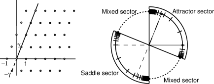
Let us now describe how to construct the sectors where the Theorem of Malmquist is valid. First of all let us consider a direction in the attractor sector that is not a singular direction of the sheaf . The sectors where the Theorem of Malmquist is valid are the sectors obtained by extending the sectors between the angles and till reach a singular direction of the sheaf (see (figure 2.6)). Since singular direction are discrete on the attracting and saddle sectors, both sectors are well defined and have amplitude greater than . Denote each one of this sectors by and .
By definition is the union of two open sets, and , contained in the attractor sector and in the saddle sector respectively. In particular . The saddle and attractor sectors, denoted by and respectively, are antipodes, i.e. . The sets and are also antipodes.
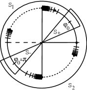
2.5.3 The importance of the pre-sheaves and
Let be the unique formal diffeomorphism of conjugating and .
Proposition 2.10
Let and be the sectors where the Theorem of Malmquist is valid. Denote by (resp. ) the normalizing application defined on (resp. ). Then, (resp. ) belongs to (resp. ).
Let (resp. ) be the restriction of to (resp. ). We have that is analytically conjugated to its formal normal form if and only if coincides with on the overlaps, i.e. if and only if both and reduces to the identity. The diffeomorphisms represents the gluing of the leaves on the overlaps. As already mentioned they take the form 2.51 with and asymptotic to zero as goes to zero.
2.5.4 Gluing of the leaves
In order to describe the gluing of the leaves on the overlaps, it is important to obtain a description of the maps of the form (2.51) on and . In other words, we shall obtain a description of the sheaves and . The next two propositions describe their fundamental properties:
Proposition 2.11
Fix a sector and assume that on . Then , for all such that .
Proof. Since the elements of are asymptotic to the Identity it follows that as goes to . Let . For a fixed the behavior of , as goes to , is given by the real part of , i.e. by .
Suppose that . Assume for a contradiction that there exists such that . Then
which means that is not asymptotic to the zero function, contradicting our assumption.
Proposition 2.12
There exists a duality between and in the following sense: if in then in . Note that by we mean the antipode of .
In particular there exists a duality between and . Therefore we just need to know the constants that can be non zero in , i.e. we need to know for which pair we have , for all such that ().
The next result expresses how the gluing of the leaves is done.
Proposition 2.13
Fix a sector and take an element of the presheaf . Thus transforms the solution of the differential equation associated to the formal normal form given by:
into the solution of the same equation given by:
where .
Fixed a sector , each represents a leaf of the foliation associated to the restriction of to . More specifically, works like a parametrization of the leaves in . If does not contain singular directions of the sheaf, we can identify with the set of transformations in the space of the leaves given by
We also denote this set by . The presheaf expresses then that the leaf of parameterized by is taken into the leaf parameterized by . Since (resp. ) does not contain singular direction of the sheaf the interpretation above can be given to the presheaf (resp. ).
Let us now explain how can be determined for a given sector . Note that are not uniquely determined and so do . The first step is to choose sectors and or, equivalently, sectors and we are going to work on. Then we consider the set of complex numbers . We can assume without loss of generality that .
Denote by the sector, with vertex at the origin, whose elements have arguments between and . Then we choose two directions not contained in such that the two of the four sectors defined by those directions do not contain any element of in its interior (figure 2.7). Fix one of those two sectors and denote it by . If is contained in the attractor sector we take otherwise we take . Note that can be chosen so close to the real axis as we want since we can chose the two directions above so close to as we want.
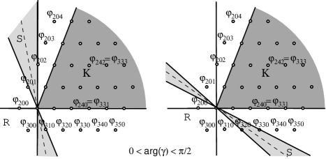
The constants that can be non zero in are those for which is in the half plane, defined by the bisectrix of , not containing . Denote this region by . For example, if we look at figure 2.7, on the left case is given by
while on the right one is given by
More specifically, the monomial coefficient of on the -component of can be non-zero if and only if . We should note that the elements of are always polynomial while the elements are always tangent to the identity, i.e, must be equal to in for all .
In the case that the constants that can be non zero in are those such that . In particular, we have only one element such that in the case of a saddle-node in dimension . Therefore the element on is just a translation as already mentioned.
Bibliography
- [Ak] D. Akhiezer, Lie group actions in complex analysis. Aspects of mathematics, E27. Friedr. Vieweg & Sohn, Braunschweig, 1995.
- [A] V. Arnold, Chapitres supplémentaires de la théorie des équations différentielles ordinaires, “Mir”, Moscow (1984)
- [Be] A. Beauville, Complex algebraic surfaces, London Math. Soc. Student Texts, 34, Cambridge University Press (1996)
- [B-M-S] M. Berthier, R. Meziani, P. Sad, On the classification of nilpotent singularities, Bull. Sci. Math. 123 (1999), no. 5, 351-370.
- [B-Mo] S. Bochner, D. Montgomery, Groups actions on analytic manifolds, Ann. of Math. (2) 48 (1947), p. 659-669.
- [C] C. Camacho, N. Kuiper, J. Palis, The topology of holomorphic flows with singularity, Publ. Math., Inst. Hautes Étud. Sci., 48, 5-38 (1978).
- [CM1] J.C. Canille Martins, Contribuição ao estudo local de fluxos holomorfos com ressonância, PhD Thesis, IMPA-CNPq, Brasil (1985)
- [CM2] J. C. Canille Martins, Holomorphic flows in with resonances, Trans. Amer. Math. Soc. 329, 825-837 (1992).
- [Car-G] L. Carleson, T.W. Gamelin Complex Dynamics, New York: Springer-Verlag, (1993) p. 174.
- [Ca-Se] H. Cartan, J-P. Serre, Un théorème de finitude concernant les variétés analytiques compactes, C. R. Acad. Sci. Paris 237, (1953), 128-130.
- [D] B. Deroin, Sur la conjecture de Remmert, Bol. Soc. Mat. Mexicana (3) 9, no. 2 (2003), 213 234.
- [E-I] P. M. Elizarov, Yu S. Il’Yashenko, Remarks in the orbital analytic classification of germs of vector fields, Math. USSR, Sb., Vol. 49, No. 1, 111-124 (1984).
- [F-Gr] K. Fritzsche, H. Grauert, From Holomorphic Functions to Complex Manifolds, Sringer (2000).
- [Fu] W. Fulton, Algebraic Curves: an Introfuction to Algebraic Geometry, Addison-Wesley Pub. (1989).
- [G-L] E. Ghys, J. Leys, Lorenz and modular flow: a visual introduction, Feature Column, AMS, Novembre 2006.
- [G-R] E. Ghys, J.-C. Rebelo, Singularités des Flots Holomorphes II, Ann. Inst. Fourier, Vol. 47, No. 4, 1117-1174 (1997).
- [G] P.A. Griffiths, Introduction to Algebraic Curves, Amer. Math. Soc. (1989) p. 225.
- [G-Ha] P.A. Griffiths, J. Harris, Principles of Algebraic Geometry, Wiley Classics Library. John Wilet & Sons Inc., New York (1994).
- [Gu] A. Guillot, Sur les équations d’Halphen et les actions de , Publ. Math. Inst. Hautes Études Sci. No. 105 (2007), 221 294.
- [H-K-M] H. Hukuara, T. Kimura, T. Matuda, Équations diférentielles ordinaires du premier ordre dans le champ complexe, Publ. Math. Soc. of Japan, 1961.
- [Ko] A. Kosinski, Differential manifolds, Dover (2007)
- [L] E.N. Lorenz, Deterministic nonperiodic flow, J. Atmosph. Sci., 20 (1963), 130-141
- [Ml] J. Malmquist, Sur l’étude analytique des solutions d’un système d’équations dans le voisinage d’ un point de indetermination, Acta Math. 73 (1941), 87-129
- [Mr] G. Marino, Equações Diferenciais Ordinárias Complexas, Master’s Thesis, PUC-Rio, Brasil (2007)
- [Ma-Ro] F. Martin, E. Royer, Formes Modulaires et Périodes. Formes modulaires et transcendance, Sémin. Congr., 12, Soc. Math. France, Paris (2005)
- [Ma-R] J. Martinet, J.-P. Ramis, Problèmes de modules pour des équations différentielles non linéaires du premier ordre, Publ. Math. I.H.E.S., 55, (1982), p.63-164.
- [M-M] J.-F. Mattei, R. Moussu, Holonomie et intégrales premières, Ann. Sc. E.N.S., IV Sér. 13 (1980), p. 469-523.
- [M] J.-F. Mattei, unpublished manuscript (1996).
- [Mu] D. Mumford, Algebraic Geometry I, Complex Projective Varieties, Springer (1976).
- [PM] R. Pérez-Marco, Solution Complète au Problème de Siegel de Linéarisation d’une Application Holomorphe au Voisinage d’un Point Fixe (D’après J.-C. Yoccoz), Sém. Bourbaki, Astérisque 206 (1992), p.273-310.
- [Re] J.-C. Rebelo, Lecture notes of a course given at Stony Brook during fall 2001.
- [R1] H. Reis Semi-complete vector fields of saddle-node type in , Trans. Amer. Math. Soc. 360, (2008), 12, 6611-6630.
- [R2] H. Reis Equivalence and semi-completude of foliations, Nonlinear Analysis, theorey, Methods and Applications, Vol. 64, No. 8, 1647-1896 (2006).
- [Sd] A. Seidenberg, Reduction of Singularities of the Differentiable Equation , Amer. J. Math., 90 (1968), p. 248-269.
- [Se] J.-P. Serre, Géométrie algébrique et géométrie analytique, Ann. Inst. Fourier, Grenoble 6 (1955-1956), 1 42.
- [Sh1] I. Shafarevich, Basic Algebraic Geometry 1, Springer (1994).
- [Sh2] I. Shafarevich, Basic Algebraic Geometry 2, Springer (1994).
- [T] W. Tucker, A rigorous ODE solver and Smale s 14th problem, Found.Comput. Math. 2, no 1 (2002), 53 117.
- [V] M. Viana, What’s new on Lorenz strange attractors, Math. Intelligencer 22-3 (2000), 6-19.
- [Vo] S. Voronin, Analytic Classification of Germs of Conformal Mappings with Identity Linear Part, Moscow State University. Translated from Funktsional’nyi Analiz i Ego Prilozheniya, vol. 15, No.1 (1981) p. 1-17.