A Matrix-Analytic Solution for Randomized Load Balancing Models with Phase-Type Service Times

Abstract

In this paper, we provide a matrix-analytic solution for randomized load balancing models (also known as supermarket models) with phase-type (PH) service times. Generalizing the service times to the phase-type distribution makes the analysis of the supermarket models more difficult and challenging than that of the exponential service time case which has been extensively discussed in the literature. We first describe the supermarket model as a system of differential vector equations, and provide a doubly exponential solution to the fixed point of the system of differential vector equations. Then we analyze the exponential convergence of the current location of the supermarket model to its fixed point. Finally, we present numerical examples to illustrate our approach and show its effectiveness in analyzing the randomized load balancing schemes with non-exponential service requirements.

1 Introduction

In the past few years, a number of companies (e.g., Amazon, Google, ,…etc) are offering the cloud computing service to enterprises. Furthermore, many content publishers and application service providers are increasingly using Data Centers to host their services. This emerging computing paradigm allows service providers and enterprises to concentrate on developing and providing their own services/goods without worrying about computing system maintenance or upgrade, and thereby significantly reduce their operating cost. For companies that offer cloud computing service in their data centers, they can take advantage of the variation of computing workloads from these customers and achieve the computational multiplexing gain. One of the important technical challenges that they have to address is how to utilize these computing resources in the data center efficiently since many of these servers can be virtualized. There is a growing interest to examine simple and robust load balancing strategies to efficiently utilize the computing resource of the server farms.

Distributed load balancing strategies, in which individual job (or customer) decisions are based on information on a limited number of other processors, have been studied analytically by Eager, Lazokwska and Zahorjan [4, 5, 6] and through trace-driven simulations by Zhou [26]. Further, randomized load balancing is a simple and effective mechanism to fairly utilize computing resources, and also can deliver surprisingly good performance measures such as reducing collisions, waiting times, backlogs,… etc. In a supermarket model, each arriving job randomly picks a small subset of servers and examines their instantaneous workload, and the job is routed to the least loaded server. When a job is committed to a server, jockeying is not allowed and each server uses the first-come-first-service (FCFS) discipline to process all jobs, e.g., see Mitzenmacher [11, 12]. For the supermarket models, most of recent research applied density dependent jump Markov processes to deal with the simple case with Poisson arrival processes and exponential service times, and illustrated that there exists a fixed point which decreases doubly exponentially. Readers may refer to, such as, a simple supermarket model by [1, 24, 11, 12]; simple variations by [19, 13, 14, 17, 23, 18, 25]; load information by [20, 3, 16, 18]; fast Jackson network by Martin and Suhov [10, 9, 21]; and general service times by Bramson, Lu and Prabhakar [2]. When the arrival processes or the service times are more general, the available results of the supermarket models are few up to now. The purpose of this paper is to provide a novel approach for studying a supermarket model with PH service times, and show that the fixed point decreases doubly exponentially.

The remainder of this paper is organized as follows. In the next section, we describe the supermarket model with the PH service times as a system of differential vector equations based on the density dependent jump Markov processes. In Section 3, we set up a system of nonlinear equations satisfied by the fixed point, provide a doubly exponential solution to the system of nonlinear equations, and compute the expected sojourn time of any arriving customer. In Section 4, we study the exponential convergence of the current location of the supermarket model to its fixed point. In Section 5, numerical examples illustrate that our approach is effective in analyzing the supermarket models from non-exponential service time requirements. Some concluding remarks are given in Section 6.

2 Supermarket Model

In this section, we describe a supermarket model with the PH service times as a system of differential vector equations based on the density dependent jump Markov processes.

Let us formally describe the supermarket model, which is abstracted as a multi-server multi-queue stochastic system. Customers arrive at a queueing system of $n>1$ servers as a Poisson process with arrival rate $n\lambda$ for $\lambda>0$. The service times of these customers are of phase type with irreducible representation $\left(\alpha,T\right)$ of order $m$. Each arriving customer chooses $d\geq 1$ servers independently and uniformly at random from these $n$ servers, and waits for service at the server which currently contains the fewest number of customers. If there is a tie, servers with the fewest number of customers will be chosen randomly. All customers in every server will be served in the FCFS manner. Please see Figure 1 for an illustration.

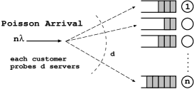
Figure 1: The supermarket model: each customer can probe the loading of $d$ servers

For the supermarket models, the PH distribution allows us to model more realistic systems and understand their performance implication under the randomized load balancing strategy. As indicated in [7], the process lifetime of many parallel jobs, in particular, jobs to data centers, tends to be non-exponential. For the PH service time distribution, we use the following irreducible representation: $\left(\alpha,T\right)$ of order $m$, the row vector $\alpha$ is a probability vector whose $j$th entry is the probability that a service begins in phase $j$ for $1\leq j\leq m$; $T$ is an $m\times m$ matrix whose $\left(i,j\right)^{th}$ entry is denoted by $t_{i,j}$ with $t_{i,i}<0$ for $1\leq i\leq m$, and $t_{i,j}\geq 0$ for $1\leq i,j\leq m$ and $i\neq j$. Let $T^{0}=-Te\gvertneqq 0$, where $e$ is a column vector of ones with a suitable dimension in the context. The expected service time is given by $1/\mu=-\alpha T^{-1}e$. Unless we state otherwise, we assume that all random variables defined above are independent, and that the system is operating in the stable region $\rho=\lambda/\mu<1$.

We define $n_{k}^{\left(i\right)}\left(t\right)$ as the number of queues with at least $k$ customers and the service time in phase $i$ at time $t\geq 0$. Clearly, $0\leq n_{k}^{\left(i\right)}\left(t\right)\leq n$ for $k\geq 0$ and $1\leq i\leq m$. Let

$$X_{n}^{\left(0\right)}\left(t\right)=\frac{n}{n}=1,$$

and $k\geq 1$

$$X_{n}^{\left(k,i\right)}\left(t\right)=\frac{n_{k}^{\left(i\right)}\left(t\right)}{n},$$

which is the fraction of queues with at least $k$ customers and the service time in phase $i$ at time $t\geq 0$. We write

$$X_{n}^{\left(k\right)}\left(t\right)=\left(X_{n}^{\left(k,1\right)}\left(t\right),X_{n}^{\left(k,2\right)}\left(t\right),\ldots,X_{n}^{\left(k,m\right)}\left(t\right)\right),\text{ \ }k\geq 1,$$

$$X_{n}\left(t\right)=\left(X_{n}^{\left(0\right)}\left(t\right),X_{n}^{\left(1\right)}\left(t\right),X_{n}^{\left(2\right)}\left(t\right),\ldots\right).$$

The state of the supermarket model may be described by the vector $X_{n}\left(t\right)$ for $t\geq 0$. Since the arrival process to the queueing system is Poisson and the service times of each server are of phase type, the stochastic process $\left\{X_{n}\left(t\right),t\geq 0\right\}$ describing the state of the supermarket model is a Markov process whose state space is given by

$$\Omega_{n} = \{\left(g_{n}^{\left(0\right)},g_{n}^{\left(1\right)},,g_{n}^{\left(2\right)}\ldots\right):g_{n}^{\left(0\right)}=1,g_{n}^{\left(k-1\right)}\geq g_{n}^{\left(k\right)}\geq 0,$$

$$\text{and \ \ }ng_{n}^{\left(k\right)}\text{ \ is a vector of nonnegative integers for }k\geq 1\}.$$

Let

$$s_{0}\left(n,t\right)=E\left[X_{n}^{\left(0\right)}\left(t\right)\right]$$

and $k\geq 1$

$$s_{k}^{\left(i\right)}\left(n,t\right)=E\left[X_{n}^{\left(k,i\right)}\left(t\right)\right].$$

Clearly, $s_{0}\left(n,t\right)=1$. We write

$$S_{k}\left(n,t\right)=\left(s_{k}^{\left(1\right)}\left(n,t\right),s_{k}^{\left(2\right)}\left(n,t\right),\ldots,s_{k}^{\left(m\right)}\left(n,t\right)\right),\text{ \ }k\geq 1.$$

As shown in Martin and Suhov [10] and Luczak and McDiarmid [8], the Markov process $\left\{X_{n}\left(t\right),t\geq 0\right\}$ is asymptotically deterministic as $n\rightarrow\infty$. Thus the limits $\lim_{n\rightarrow\infty}E\left[X_{n}^{\left(0\right)}\left(t\right)\right]$ and $\lim_{n\rightarrow\infty}E\left[X_{n}^{\left(k,i\right)}\right]$ always exist by means of the law of large numbers. Based on this, we write

$$S_{0}\left(t\right)=\lim_{n\rightarrow\infty}s_{0}\left(n,t\right)=1,$$

for $k\geq 1$

$$s_{k}^{\left(i\right)}\left(t\right)=\lim_{n\rightarrow\infty}s_{k}^{\left(i\right)}\left(n,t\right),$$

$$S_{k}\left(t\right)=\left(s_{k}^{\left(1\right)}\left(t\right),s_{k}^{\left(2\right)}\left(t\right),\ldots,s_{k}^{\left(m\right)}\left(t\right)\right)$$

and

$$S\left(t\right)=\left(S_{0}\left(t\right),S_{1}\left(t\right),S_{2}\left(t\right),\ldots\right).$$

Let $X\left(t\right)=\lim_{n\rightarrow\infty}X_{n}\left(t\right)$. Then it is easy to see from the Poisson arrivals and the PH service times that $\left\{X\left(t\right),t\geq 0\right\}$ is also a Markov process whose state space is given by

$$\Omega=\left\{\left(g^{\left(0\right)},g^{\left(1\right)},g^{\left(2\right)},\ldots\right):g^{\left(0\right)}=1,g^{\left(k-1\right)}\geq g^{\left(k\right)}\geq 0\right\}.$$

If the initial distribution of the Markov process $\left\{X_{n}\left(t\right),t\geq 0\right\}$ approaches the Dirac delta-measure concentrated at a point $g\in$ $\Omega$, then its steady-state distribution is concentrated in the limit on the trajectory $S_{g}=\left\{S\left(t\right):t\geq 0\right\}$. This indicates a law of large numbers for the time evolution of the fraction of queues of different lengths. Furthermore, the Markov process $\left\{X_{n}\left(t\right),t\geq 0\right\}$ converges weakly to the fraction vector $S\left(t\right)=\left(S_{0}\left(t\right),S_{1}\left(t\right),S_{2}\left(t\right),\ldots\right)$, or for a sufficiently small $\varepsilon>0$,

$$\lim_{n\rightarrow\infty}P\left\{||X_{n}\left(t\right)-S\left(t\right)||\geq\varepsilon\right\}=0,$$

where $||a||$ is the $L_{\infty}$-norm of vector $a$.

In what follows we provide a system of differential vector equations in order to determine fraction vector $S\left(t\right)$. To that end, we introduce the Hadamard Product of two matrices $A=\left(a_{i,j}\right)$ and $B=\left(b_{i,j}\right)$ as follows:

$$A\odot B=\left(a_{i,j}b_{i,j}\right).$$

Specifically, for $k\geq 2$, we have

$$A^{\odot k}=\underset{k\text{ matrix }A}{\underbrace{A\odot A\odot\cdots\odot A}}.$$

To determine the fraction vector $S\left(t\right)$, we need to set up a system of differential vector equations satisfied by $S\left(t\right)$ by means of the density dependent jump Markov process. To that end, we provide a concrete example for $k\geq 2$ to indicate how to derive the the system of differential vector equations.

Consider the supermarket model with $n$ servers, and determine the expected change in the number of queues with at least $k$ customers over a small time period of length d$t$. The probability vector that during this time period, any arriving customer joins a queue of size $k-1$ is given by

$$n\left[\lambda S_{k-1}^{\odot d}\left(n,t\right)-\lambda S_{k}^{\odot d}\left(n,t\right)\right]\text{d}t.$$

Similarly, the probability vector that a customer leaves a server queued by $k$ customers is given by

$$n\left[S_{k}\left(n,t\right)T+S_{k+1}\left(n,t\right)T^{0}\alpha\right]\text{d}t.$$

Therefore we can obtain

$$\text{d}E\left[n_{k}\left(n,t\right)\right]= n\left[\lambda S_{k-1}^{\odot d}\left(n,t\right)-\lambda S_{k}^{\odot d}\left(n,t\right)\right]\text{d}t$$

$$+n\left[S_{k}\left(n,t\right)T+S_{k+1}\left(n,t\right)T^{0}\alpha\right]\text{d}t,$$

which leads to

$$\frac{\text{d}S_{k}\left(n,t\right)}{\text{d}t}=\lambda S_{k-1}^{\odot d}\left(n,t\right)-\lambda S_{k}^{\odot d}\left(n,t\right)+S_{k}\left(n,t\right)T+S_{k+1}\left(n,t\right)T^{0}\alpha.$$

Taking $n\rightarrow\infty$ in the both sides of Equation (LABEL:Equ1), we have

$$\frac{\text{d}S_{k}\left(t\right)}{\text{d}t}=\lambda S_{k-1}^{\odot d}\left(t\right)-\lambda S_{k}^{\odot d}\left(t\right)+S_{k}\left(t\right)T+S_{k+1}\left(t\right)T^{0}\alpha.$$

Using a similar analysis to Equation (LABEL:Equ2), we can obtain a system of differential vector equations for the fraction vector $S\left(t\right)=\left(S_{0}\left(t\right),S_{1}\left(t\right),S_{2}\left(t\right),\ldots\right)$ as follows:

$$S_{0}\left(t\right)=1,$$

$$\frac{\mathtt{d}}{\text{d}t}S_{0}\left(t\right)=-\lambda S_{0}^{d}\left(t\right)+S_{1}\left(t\right)T^{0},$$ (1)

$$\frac{\mathtt{d}}{\text{d}t}S_{1}\left(t\right)=\lambda\alpha S_{0}^{d}\left(t\right)-\lambda S_{1}^{\odot d}\left(t\right)+S_{1}\left(t\right)T+S_{2}\left(t\right)T^{0}\alpha,$$ (2)

and for $k\geq 2$,

$$\frac{\mathtt{d}}{\text{d}t}S_{k}\left(t\right)=\lambda S_{k-1}^{\odot d}\left(t\right)-\lambda S_{k}^{\odot d}\left(t\right)+S_{k}\left(t\right)T+S_{k+1}\left(t\right)T^{0}\alpha.$$ (3)

Remark 1

Mitzenmacher [11, 12] provided an heuristical and interesting method to establish such systems of differential equations, but they lack a rigorous mathematical meaning for understanding the stochastic process $\left\{X_{n}\left(t\right),t\geq 0\right\}$ in which $X_{n}\left(t\right)=(X_{n}^{\left(0\right)}\left(t\right),X_{n}^{\left(1\right)}\left(t\right),$ $X_{n}^{\left(2\right)}\left(t\right),\ldots)$ and $X_{n}^{\left(k\right)}\left(t\right)=n_{k}\left(t\right)/n$ for $k\geq 0$. This section, following Martin and Suhov [10] and Luczak and McDiarmid [8], gives some necessary mathematical analysis for the stochastic process $\left\{X_{n}\left(t\right),t\geq 0\right\}$ and the system of differential vector equations (1), (2) and (3).

3 A Matrix-Analytic Solution

In this section, we provide a doubly exponential solution to the fixed point of the system of differential vector equations (1), (2) and (3).

A row vector $\pi=\left(\pi_{0},\pi_{1},\pi_{2},\ldots\right)$ is called a fixed point of the fraction vector $S\left(t\right)$ if $\lim_{t\rightarrow+\infty}S\left(t\right)=\pi$. In this case, it is easy to see that

$$\lim_{t\rightarrow+\infty}\left[\frac{\mathtt{d}}{\text{d}t}S\left(t\right)\right]=0.$$

Therefore, as $t\rightarrow+\infty$ the system of differential vector equations (1), (2) and (3) can be simplified as

$$-\lambda\pi_{0}^{d}+\pi_{1}T^{0}=0,$$ (4)

$$\lambda\alpha\pi_{0}^{d}-\lambda\pi_{1}^{\odot d}+\pi_{1}T+\pi_{2}T^{0}\alpha=0,$$ (5)

and for $k\geq 2$,

$$\lambda\pi_{k-1}^{\odot d}-\lambda\pi_{k}^{\odot d}+\pi_{k}T+\pi_{k+1}T^{0}\alpha=0.$$ (6)

In general, it is more difficult and challenging to express the fixed point of the supermarket models with more general arrival processes or service times, because the systems of nonlinear equations are more complicated for computation. Fortunately, we can derive a closed-form expression for the fixed point $\pi=(\pi_{0},\pi_{1},\pi_{2},...)$ for the supermarket model with PH service times by means of a novel matrix-analytic approach given as follows.

Noting that $S_{0}\left(t\right)=1$ for all $t\geq 0$, it is easy to see that $\pi_{0}=1$. It follows from Equation (4) that

$$\pi_{1}T^{0}=\lambda.$$ (7)

To solve Equation (7), we denote by $\omega$ the stationary probability vector of the irreducible Markov chain $T+T^{0}\alpha$. Obviously, we have

$$\omega T^{0}=\mu,$$

$$\frac{\lambda}{\mu}\omega T^{0}=\lambda.$$ (8)

Thus, we obtain $\pi_{1}=\frac{\lambda}{\mu}\omega=\rho\cdot\omega$. Based on the fact that $\pi_{0}=1$ and $\pi_{1}=\rho\cdot\omega$, it follows from Equation (5) that

$$\lambda\alpha-\lambda\rho^{d}\cdot\omega^{\odot d}+\rho\cdot\omega T+\pi_{2}T^{0}\alpha=0,$$

which leads to

$$\lambda-\lambda\rho^{d}\cdot\omega^{\odot d}e+\rho\cdot\omega Te+\pi_{2}T^{0}=0.$$

Note that $\omega Te=-\mu$, we obtain

$$\pi_{2}T^{0}=\lambda\rho^{d}\omega^{\odot d}e.$$

Let $\theta=\omega^{\odot d}e$. Then it is easy to see that $\theta\in\left(0,1\right)$, and

$$\pi_{2}T^{0}=\lambda\theta\rho^{d}.$$

Using a similar analysis to Equation (8), we have

$$\pi_{2}=\frac{\lambda\theta\rho^{d}}{\mu}\omega=\theta\rho^{d+1}\cdot\omega.$$ (9)

Based on $\pi_{1}=\rho\cdot\omega$ and $\pi_{2}=\theta\rho^{d+1}\cdot\omega$, it follows from Equation (6) that for $k=2$,

$$\lambda\rho^{d}\cdot\omega^{\odot d}-\lambda\theta^{d}\rho^{d^{2}+d}\cdot\omega^{\odot d}+\theta\rho^{d+1}\cdot\omega T+\pi_{3}T^{0}\alpha=0,$$

which leads to

$$\lambda\theta\rho^{d}-\lambda\theta^{d+1}\rho^{d^{2}+d}+\theta\rho^{d+1}\cdot\omega Te+\pi_{3}T^{0}=0,$$

thus we obtain

$$\pi_{3}T^{0}=\lambda\theta^{d+1}\rho^{d^{2}+d}.$$

Using a similar analysis on Equation (8), we have

$$\pi_{3}=\frac{\lambda\theta^{d+1}\rho^{d^{2}+d}}{\mu}\omega=\theta^{d+1}\rho^{d^{2}+d+1}\cdot\omega.$$ (10)

Based on Equations (9) and (10), we may infer that there is a structured expression $\pi_{k}=\theta^{d^{k-2}+d^{k-3}+\cdots+d+1}\rho^{d^{k-1}+d^{k-2}+\cdots+d+1}\cdot\omega$, for $k\geq 1$. To that end, the following theorem states this important result.

Theorem 1

The fixed point $\pi=\left(\pi_{0},\pi_{1},\pi_{2},\ldots\right)$ is unique and is given by

$$\pi_{0}=1,\hskip 14.45377pt\pi_{1}=\rho\cdot\omega$$

and for $k\geq 2,$

$$\pi_{k}=\theta^{d^{k-2}+d^{k-3}+\cdots+1}\rho^{d^{k-1}+d^{k-2}+\cdots+1}\cdot\omega,$$ (11)

or

$$\pi_{k} = \theta^{\frac{d^{k-1}-1}{d-1}}\rho^{\frac{d^{k}-1}{d-1}}\cdot\omega=\rho^{d^{k-1}}\left(\theta\rho\right)^{\frac{d^{k-1}-1}{d-1}}\cdot\omega.$$

Proof: By induction, one can easily derive the above result.

It is clear that Equation (11) is correct for the cases with $l=2,3$ according to Equations (9) and (10). Now, we assume that Equation (11) is correct for the cases with $l=k$. Then it follows from Equation (6) that for $l=k+1$, we have

$$\lambda \theta^{d^{k-2}+d^{k-3}+\cdots+d}\rho^{d^{k-1}+d^{k-2}+\cdots+d}\cdot\omega^{\odot d}-\lambda\theta^{d^{k-1}+d^{k-2}+\cdots+d}\rho^{d^{k}+d^{k-1}+\cdots+d}\cdot\omega^{\odot d}$$

$$+\theta^{d^{k-2}+d^{k-3}+\cdots+1}\rho^{d^{k-1}+d^{k-2}+\cdots+1}\cdot\omega T+\pi_{k+1}T^{0}\alpha=0,$$

which leads to

$$\lambda \theta^{d^{k-2}+d^{k-3}+\cdots+d+1}\rho^{d^{k-1}+d^{k-2}+\cdots+d}-\lambda\theta^{d^{k-1}+d^{k-2}+\cdots+d+1}\rho^{d^{k}+d^{k-1}+\cdots+d}$$

$$+\theta^{d^{k-2}+d^{k-3}+\cdots+1}\rho^{d^{k-1}+d^{k-2}+\cdots+1}\cdot\omega Te+\pi_{k+1}T^{0}=0,$$

thus we obtain

$$\pi_{k+1}T^{0}=\lambda\theta^{d^{k-1}+d^{k-2}+\cdots+d+1}\rho^{d^{k}+d^{k-1}+\cdots+d}.$$

By a similar analysis to (8), we have

$$\pi_{k+1} =\frac{\lambda\theta^{d^{k-1}+d^{k-2}+\cdots+d+1}\rho^{d^{k}+d^{k-1}+\cdots+d}}{\mu}\omega$$

$$=\theta^{d^{k-1}+d^{k-2}+\cdots+d+1}\rho^{d^{k}+d^{k-1}+\cdots+d+1}\cdot\omega.$$

This completes the proof.  

Now, we compute the expected sojourn time $T_{d}$ that a tagged arriving customer spends in the supermarket model. For the PH service times, a tagged arriving customer is the $k$th customer in the corresponding queue with probability vector $\pi_{k-1}^{\odot d}-\pi_{k}^{\odot d}$. When $k\geq 1$, the head customer in the queue has been served, and so its service time is residual and is denoted as $X_{R}$. Let $X$ be of phase type with irreducible representation $\left(\alpha,T\right)$. Then $X_{R}$ is of phase type with irreducible representation $\left(\omega,T\right)$. Clearly, we have

$$E\left[X\right]=\alpha\left(-T\right)^{-1}e,\text{ \ }E\left[X_{R}\right]=\omega\left(-T\right)^{-1}e.$$

Thus it is easy to see that the expected sojourn time of the tagged arriving customer is given by

$$E\left[T_{d}\right] =\left(\pi_{0}^{d}-\pi_{1}^{\odot d}e\right)E\left[X\right]+\sum_{k=1}^{\infty}\left(\pi_{k}^{\odot d}-\pi_{k+1}^{\odot d}\right)e\left\{E\left[X_{R}\right]+kE\left[X\right]\right\}$$

$$=\pi_{1}^{\odot d}e\left\{E\left[X_{R}\right]-E\left[X\right]\right\}+E\left[X\right]\left[1+\sum_{k=1}^{\infty}\pi_{k}^{\odot d}e\right]$$

$$=\rho^{d}\theta\left(\omega-\alpha\right)\left(-T\right)^{-1}e+\alpha\left(-T\right)^{-1}e\left(1+\sum_{k=1}^{\infty}\theta^{\frac{d^{k}-1}{d-1}}\rho^{\frac{d^{k+1}-d}{d-1}}\right).$$

When the arrival process and the service time distribution are Poisson and exponential, respectively, it is clear that $\alpha=\omega=\theta=1$ and $\alpha\left(-T\right)^{-1}e=1/\mu$, thus we have

$$E\left[T_{d}\right]=\frac{1}{\mu}\sum_{k=0}^{\infty}\rho^{\frac{d^{k+1}-d}{d-1}},$$

which is the same as Corollary 3.8 in Mitzenmacher [12].

In what follows we consider an interesting problem: how many moments of the service time distribution are needed to obtain a better accuracy for computing the fixed point or the expected sojourn time. It is well-known from the theory of probability distributions that the first three moments is basic for analyzing such an accuracy, and we can construct a PH distribution of order 2 by using the first three moments. Telek and Heindl [22] provided a fitting procedure for matching a PH distribution of order 2 from the first three moments exactly. It is necessary to list the fitting procedure as follows:

For a nonnegative random variable $X$, let $m_{n}=E\left[X^{n}\right]$, $n\geq 1$. We take a PH distribution of order 2 with the canonical representation $\left(\alpha,T\right)$, where $\mathbf{\alpha=}\left(\eta,1-\eta\right)$ and

$$T\mathbf{=}\left(\begin{array}[]{cc}-\xi_{1}&\xi_{1}\\ 0&-\xi_{2}\end{array}\right),$$

$0\leq\eta\leq 1$ and $0<\xi_{1}\leq\xi_{2}$. Note that the three unknown parameters $\eta$, $\xi_{1}$ and $\xi_{2}$ can be obtained from the first three moments $m_{1}$, $m_{2}$ and $m_{3}$ of an arbitrary general distribution.

Table 1: Specific Bounds of the First Three Moments

Moment	Condition	Bounds
$m_{1}$		$0<m_{1}<\infty$
$m_{2}$		$1.5m_{1}^{2}\leq m_{2}$
$m_{3}$	$0.5\leq c_{X}^{2}\leq 1$	$3m_{1}^{3}\left(3c_{X}^{2}-1+\sqrt{2}\left(1-c_{X}^{2}\right)^{\frac{3}{2}}\right)\leq m_{3}\leq 6m_{1}^{3}c_{X}^{2}$
	$1<c_{X}^{2}$	$\frac{3}{2}m_{1}^{3}\left(1+c_{X}^{2}\right)^{2}<m_{3}<\infty$

In Table 1, $c_{X}^{2}=m_{2}\diagup m_{1}^{2}-1$ is the squared coefficient of variation. If the moments do not satisfy these conditions in Table 1, then we may analyze the following four cases:

(a.1) if $m_{2}<1.5m_{1}^{2}$, then we take $m_{2}=1.5m_{1}^{2}$;

(a.2) if $0.5\leq c_{X}^{2}\leq 1$, and $m_{3}<3m_{1}^{3}\left(3c_{X}^{2}-1+\sqrt{2}\left(1-c_{X}^{2}\right)^{\frac{3}{2}}\right)$, then we take $m_{3}=3m_{1}^{3}\left(3c_{X}^{2}-1+\sqrt{2}\left(1-c_{X}^{2}\right)^{\frac{3}{2}}\right)$;

(a.3) if $0.5\leq c_{X}^{2}\leq 1$, and $m_{3}>6m_{1}^{3}c_{X}^{2}$, then we take $m_{3}=6m_{1}^{3}c_{X}^{2}$; and

(a.4) if $1<c_{X}^{2}$, and $m_{3}\leq\frac{3}{2}m_{1}^{3}\left(1+c_{X}^{2}\right)^{2}$, then we take $m_{3}=\frac{3}{2}m_{1}^{3}\left(1+c_{X}^{2}\right)^{2}$.

Let $c=3m_{2}^{2}-2m_{1}m_{3}$, $d=2m_{1}^{2}-m_{2}$, $b=3m_{1}m_{2}-m_{3}$ and $a=b^{2}-6cd$. If the moments respectively satisfy their specific bounds shown in Table 1 or the exceptive four cases, then three unknown parameters $\eta$, $\xi_{1}$ and $\xi_{2}$ can be computed in the following three cases.

(1) If $c>0$, then

$$\eta=\frac{-b+6m_{1}d+\sqrt{a}}{b+\sqrt{a}},\text{ }\xi_{1}=\frac{b-\sqrt{a}}{c},\text{ }\xi_{2}=\frac{b+\sqrt{a}}{c}.$$

(2) If $c<0$, then

$$\eta=\frac{b-6m_{1}d+\sqrt{a}}{-b+\sqrt{a}},\text{ }\xi_{1}=\frac{b+\sqrt{a}}{c},\text{ }\xi_{2}=\frac{b-\sqrt{a}}{c}.$$

(3) If $c=0$, then

$$\eta=0,\text{ }\xi_{1}>0,\text{ }\xi_{2}=\frac{1}{m_{1}}.$$

From the above discussion, we can always construct a PH distribution of order 2 to approximate an arbitrary general distribution with the same first three moments. In fact, such an approximation achieves a better accuracy in computation.

For the PH distribution of order 2, we have

$$T+T^{0}\alpha=\left(\begin{array}[]{cc}-\xi_{1}&\xi_{1}\\ 0&-\xi_{2}\end{array}\right)+\left(\begin{array}[]{c}0\\ \xi_{2}\end{array}\right)\left(\begin{array}[]{cc}\eta&1-\eta\end{array}\right)=\left(\begin{array}[]{cc}-\xi_{1}&\xi_{1}\\ \xi_{2}\eta&-\xi_{2}\eta\end{array}\right),$$

which leads to

$$\omega=\left(\frac{\xi_{2}\eta}{\xi_{1}+\xi_{2}\eta},\frac{\xi_{1}}{\xi_{1}+\xi_{2}\eta}\right)$$

and

$$\theta=\frac{\xi_{1}^{d}+\xi_{2}^{d}\eta^{d}}{\left(\xi_{1}+\xi_{2}\eta\right)^{d}}.$$

Thus, the PH distribution of order 2 can effectively approximates an arbitrary general service time distribution in the supermarket model under the same first three moments, and specifically, all the computations are very simple to implement.

Remark 2

Bramson, Lu and Prabhakar [2] provided a modularized program based on ansatz for treating the supermarket model with a general service time distribution. They organized a functional equation $\pi=F\left(G\left(\pi\right)\right)$ for analyzing the stationary probability vector $\pi$ in terms of insensitivity and generalized Fibonacci sequences, although the operators $F$ and $G$ are not easy to be given for this supermarket model. This paper studies the supermarket model with a PH service time distribution, provides the doubly exponential solution to the fixed point, and is specifically related to the phase type environment by means of the crucial factor $\theta=\omega^{\odot d}e$. Note that the PH distributions are dense in the set of all nonnegative random variables, this paper can numerically provide necessary understanding for the role played by the general service time distribution in performance analysis of the supermarket model by means of the PH approximation of order 2.

4 Exponential convergence to the fixed point

In this section, we study the exponential convergence of the current location $S\left(t\right)$ of the supermarket model to its fixed point $\pi$.

For the supermarket model, the initial point $S\left(0\right)$ can affect the current location $S\left(t\right)$ for each $t>0$, since the service process in the supermarket model is under a unified structure. To that end, we provide some notation for comparison of two vectors. Let $a=\left(a_{1},a_{2},a_{3},\ldots\right)$ and $b=\left(b_{1},b_{2},b_{3},\ldots\right)$. We write $a\prec b$ if $a_{k}<b_{k}$ for some $k\geq 1$ and $a_{l}\leq b_{l}$ for $l\neq k,l\geq 1$; and $a\preceq b$ if $a_{k}\leq b_{k}$ for all $k\geq 1$. Now, we can obtain the following useful proposition whose proof is clear from a sample path analysis and thus is omitted here.

Proposition 1

If $S\left(0\right)\preceq\widetilde{S}\left(0\right)$, then $S\left(t\right)\preceq\widetilde{S}\left(t\right)$.

Based on Proposition 1, the following theorem shows that the fixed point $\pi$ is an upper bound of the current location $S\left(t\right)$ for all $t\geq 0$.

Theorem 2

For the supermarket model, if there exists some $k$ such that $S_{k}\left(0\right)=0$, then the sequence $\left\{S_{k}\left(t\right)\right\}$ has an upper bound sequence which decreases doubly exponentially for all $t\geq 0$, that is, $S\left(t\right)\preceq\pi$ for all $t\geq 0$.

Proof:  Let $\widetilde{S}_{k}\left(0\right)=\pi_{k}$ for $k\geq 1$. Then for each $k\geq 1$, $\widetilde{S}_{k}\left(t\right)=\widetilde{S}_{k}\left(0\right)=\pi_{k}$ for all $t\geq 0$, since $\widetilde{S}\left(0\right)=\left(\widetilde{S}_{1}\left(0\right),\widetilde{S}_{2}\left(0\right),\widetilde{S}_{2}\left(0\right),\ldots\right)$ is a fixed point in the supermarket model. If $S_{k}\left(0\right)=0$ for some $k$, then $S_{k}\left(0\right)\prec\widetilde{S}_{k}\left(0\right)$ and $S_{j}\left(0\right)\preceq\widetilde{S}_{j}\left(0\right)$ for $j\neq k,j\geq 1$, thus $S\left(0\right)\preceq\widetilde{S}\left(0\right)$. It is easy to see from Proposition 1 that $S_{k}\left(t\right)\preceq\widetilde{S}_{k}\left(t\right)=\pi_{k}$ for all $k\geq 1$ and $t\geq 0$. Thus we obtain that for all $k\geq 1$ and $t\geq 0$

$$S_{k}\left(t\right)\leq\theta^{\frac{d^{k-1}-1}{d-1}}\rho^{\frac{d^{k}-1}{d-1}}\cdot\omega.$$

This completes the proof.  

To show the exponential convergence, we define a Lyapunov function $\Phi\left(t\right)$ as

$$\Phi\left(t\right)=\sum_{k=1}^{\infty}w_{k}\left[\pi_{k}-S_{k}\left(t\right)\right]e$$

in terms of the fact that $S_{k}\left(t\right)\preceq\pi_{k}$ for $k\geq 1$ and $\pi_{0}=S_{0}\left(t\right)=1$, where $\left\{w_{k}\right\}$ is a positive scalar sequence with $w_{k+1}\geq w_{k}\geq w_{1}=1$ for $k\geq 2$.

The following theorem measures the distance $\Phi\left(t\right)$ of the current location $S\left(t\right)$ for $t\geq 0$ to the fixed point $\pi$, and illustrates that this distance between the fixed point and the current location is very close to zero with exponential convergence. This shows that from a suitable starting point, the supermarket model can be quickly close to the fixed point.

Theorem 3

For $t\geq 0$, $\Phi\left(t\right)\leq c_{0}e^{-\delta t}$, where $c_{0}$ and $\delta$ are two positive constants. In this case, the potential function $\Phi\left(t\right)$ is exponentially convergent.

Proof:  Note that

$$\Phi\left(t\right)=\sum_{k=1}^{\infty}w_{k}\left[\pi_{k}-S_{k}\left(t\right)\right]e,$$

we have

$$\frac{d}{dt}\Phi\left(t\right)=-\sum_{k=1}^{\infty}w_{k}\frac{d}{dt}S_{k}\left(t\right)e.$$

It follows from Equations (1) to (3) that

$$\frac{d}{dt}\Phi\left(t\right)= -w_{1}[\lambda S_{0}^{d}\left(t\right)\alpha-\lambda S_{1}^{\odot d}\left(t\right)+S_{1}\left(t\right)T+S_{2}\left(t\right)T^{0}\alpha]e$$

$$-\sum_{k=1}^{\infty}w_{k}[\lambda S_{k-1}^{\odot d}\left(t\right)-\lambda S_{k}^{\odot d}\left(t\right)+S_{k}\left(t\right)T+S_{k+1}\left(t\right)T^{0}\alpha]e.$$

By means of $S_{0}\left(t\right)=1$ and $Te=-T^{0}$, we can obtain

$$\frac{d}{dt}\Phi\left(t\right)= -w_{1}[\lambda-\lambda S_{1}^{\odot d}\left(t\right)e-S_{1}\left(t\right)T^{0}+S_{2}\left(t\right)T^{0}]$$

$$-\sum_{k=2}^{\infty}w_{k}[\lambda S_{k-1}^{\odot d}\left(t\right)e-\lambda S_{k}^{\odot d}\left(t\right)e-S_{k}\left(t\right)T^{0}+S_{k+1}\left(t\right)T^{0}].$$ (12)

We take some nonnegative constants $c_{k}\left(t\right)$ and $d_{k}\left(t\right)$ for $k\geq 1$ such that

$$\lambda=f_{1}\left(t\right)S_{1}\left(t\right)T^{0},$$

for $k\geq 1$

$$\lambda S_{k}^{\odot d}\left(t\right)e=c_{k}\left(t\right)\left[\pi_{k}-S_{k}\left(t\right)\right]e$$

and

$$S_{k}\left(t\right)T^{0}=d_{k}\left(t\right)\left[\pi_{k}-S_{k}\left(t\right)\right]e.$$

Then it follows from (12) that

$$\frac{d}{dt}\Phi\left(t\right) =-\left\{\left[\left(w_{2}-w_{1}\right)\right]c_{1}\left(t\right)+w_{1}\left[f_{1}\left(t\right)-1\right]d_{1}\left(t\right)\right\}\cdot\left[\pi_{1}-S_{1}\left(t\right)\right]e$$

$$-\sum_{k=2}^{\infty}\left[\left(w_{k+1}-w_{k}\right)c_{k}\left(t\right)+\left(w_{k-1}-w_{k}\right)d_{k}\left(t\right)\right]\cdot\left[\pi_{k}-S_{k}\left(t\right)\right]e.$$

For a constant $\delta>0$, we take

$$w_{1}=1,$$

$$\left[\left(w_{2}-w_{1}\right)\right]c_{1}\left(t\right)+w_{1}\left[f_{1}\left(t\right)-1\right]d_{1}\left(t\right)\geq\delta w_{1}$$

and

$$\left(w_{k+1}-w_{k}\right)c_{k}\left(t\right)+\left(w_{k-1}-w_{k}\right)d_{k}\left(t\right)\geq\delta w_{k}.$$

In this case, it is easy to see that

$$w_{2}\geq 1+\frac{\delta+1-f_{1}\left(t\right)}{c_{1}\left(t\right)}$$

and for $k\geq 2$

$$w_{k+1}\geq w_{k}+\frac{\delta w_{k}}{c_{k}\left(t\right)}+\frac{d_{k}\left(t\right)}{c_{k}\left(t\right)}\left(w_{k}-w_{k-1}\right).$$

Thus we have

$$\frac{d}{dt}\Phi\left(t\right)\leq-\delta\sum_{k=0}^{\infty}w_{k}\left[\pi_{k}-S_{k}\left(t\right)\right]e=-\delta\Phi\left(t\right),$$

which can leads to

$$\Phi\left(t\right)\leq c_{0}e^{-\delta t}.$$

This completes the proof.  

5 Numerical examples

In this section, we provide some numerical examples to illustrate that our approach is effective and efficient in the study of supermarket models with non-exponential service requirements, including Erlang service time distributions, hyper-exponential service time distributions and PH service time distributions.

Example one (Erlang Distribution) We consider an $m$-order Erlang distribution with the irreducible PH representation $(\alpha,T)$, where$\alpha=\left(1,0,\ldots,0,0\right)$ and

$$T=\left(\begin{array}[]{ccccc}-\eta&\eta&&&\\ &-\eta&\eta&&\\ &&\ddots&\ddots&\\ &&&-\eta&\eta\\ &&&&-\eta\end{array}\right),\text{ \ \ }T^{0}=\left(\begin{array}[]{c}0\\ 0\\ \vdots\\ 0\\ \eta\end{array}\right).$$

It is clear that

$$T+T^{0}\alpha=\left(\begin{array}[]{ccccc}-\eta&\eta&&&\\ &-\eta&\eta&&\\ &&\ddots&\ddots&\\ &&&-\eta&\eta\\ \eta&&&&-\eta\end{array}\right),$$

which leads to the stationary probability vector of the Markov chain $T+T^{0}\alpha$ as follows:

$$\omega=\left(\frac{1}{m},\frac{1}{m},\ldots\frac{1}{m},\frac{1}{m}\right);\hskip 7.22743pt\mu=\omega T^{0}=\frac{\eta}{m};\hskip 7.22743pt\rho=\frac{\lambda}{\mu}=\frac{m\lambda}{\eta};\hskip 7.22743pt\theta=m\left(\frac{1}{m}\right)^{d}=m^{1-d}.$$

Thus we obtain

$$\pi_{k} =m^{1-d^{k-1}}\left(\frac{m\lambda}{\eta}\right)^{\frac{d^{k}-1}{d-1}}\left(\frac{1}{m},\frac{1}{m},\ldots\frac{1}{m},\frac{1}{m}\right)$$

$$=m^{\frac{d^{k-1}+d-2}{d-1}}\left(\frac{\lambda}{\eta}\right)^{\frac{d^{k}-1}{d-1}}\left(\frac{1}{m},\frac{1}{m},\ldots\frac{1}{m},\frac{1}{m}\right).$$

Let $\lambda=1$. If $\rho=\frac{m\lambda}{\eta}<1$, then this supermarket model is stable. In the stable case, $\eta>m$. We may consider the following simple cases:
(a) If $m=2$ and $d=2$, then $\pi_{k}=2^{2^{k-1}}\eta^{1-2^{k}}$.

(b) If $m=3$ and $d=2$, then $\pi_{k}=3^{2^{k-1}}\eta^{1-2^{k}}$.

Based on the two simple examples with $\lambda=1$ and $d=2$, we need to illustrate how the fixed point depends on the stage number $m$ and the exponential service rate $\eta$. To that end, we write $\pi_{k}\left(m,\eta\right)$. It is easy to see that for a given pair $\left(k,\eta\right)$ for $\eta>m$ and $k=1,2,\ldots,$ we have

$$\pi_{k}\left(1,\eta\right)<\pi_{k}\left(2,\eta\right)<\cdots<\pi_{k}\left(m,\eta\right)<\cdots.$$

On the other hand, for a given pair $\left(k,m\right)$ for $m,k=1,2,\ldots,$ we can see that $\pi_{k}\left(m,\eta\right)$ is a decreasing function of $\eta$.

Let us consider the average response time of the supermarket model with an $m-$stage Erlang distribution. We first consider a parallel system with $n=100$ servers and the service time distribution is exponential. We normalize the average service time to unity and vary the arrival rate $\lambda$. For the $m-$stage Erlang distribution, the bigger the number $m$ is, the bigger its variance is. Table 2 illustrates the average response time under different probe size $d$. One can observe that there is a dramatic improvement (or reduction) in the average response time when increasing the probe size $d$.

Table 2: Average response time for exponential service time

number of servers ($n$)	probe size ($d$)	arrival rate ($\lambda$)	response time ($E[\mathcal{T}]$)
100	2	0.500000	1.395977
100	2	0.700000	1.768194
100	2	0.800000	2.072020
100	2	0.900000	2.721852
100	3	0.500000	1.395320
100	3	0.700000	1.604113
100	3	0.800000	1.802933
100	3	0.900000	2.209601
100	5	0.900000	1.916280

We further analyze the cases that the service time is either distributed according to $2$-stage Erlang or $3$-stage Erlang distribution. Similarly, we normalized the total average service time as unity and we vary the arrival rate $\lambda$. Tables 3 and 4 illustrate the average response time under different probe size $d$. One can observe that

• Simple probing size $d$ can significantly improve the performance by lowering the average response time.

• When the service time has lower variance, the average response time is lower.

Table 3: Average response time for $2-$stage Erlang service time

number of servers ($n$)	probe size ($d$)	arrival rate ($\lambda$)	response time ($E[\mathcal{T}]$)
100	2	0.500000	1.353783
100	2	0.700000	1.599851
100	2	0.800000	1.829199
100	2	0.900000	2.298470
100	3	0.500000	1.325610
100	3	0.700000	1.492651
100	3	0.800000	1.639987
100	3	0.900000	1.941196
100	5	0.900000	1.739867

Table 4: Average response time for $3-$stage Erlang service time

number of servers ($n$)	probe size ($d$)	arrival rate ($\lambda$)	response time ($E[\mathcal{T}]$)
100	2	0.500000	1.322544
100	2	0.700000	1.539621
100	2	0.800000	1.739972
100	2	0.900000	2.148191
100	3	0.500000	1.298863
100	3	0.700000	1.452785
100	3	0.800000	1.581663
100	3	0.900000	1.834704
100	5	0.900000	1.678233

Example two (Hyper-Exponential Distribution) We consider an $m$-order hyper-exponential distribution $F\left(x\right)=1-\sum\limits_{k=1}^{m}\alpha_{k}\exp\left\{-\eta_{k}x\right\}$, or the probability density function $f\left(x\right)=\sum\limits_{k=1}^{m}\alpha_{k}\eta_{k}\exp\left\{-\eta_{k}x\right\}$. It is clear that the hyper-exponential distribution is of phase type with the irreducible representation $(\alpha,T)$, where $\alpha=\left(\alpha_{1},\alpha_{2},\ldots,\alpha_{m}\right)$, and

$$T=\left(\begin{array}[]{cccc}-\eta_{1}&&&\\ &-\eta_{2}&&\\ &&\ddots&\\ &&&-\eta_{m}\end{array}\right),\text{ \ }T^{0}=\left(\begin{array}[]{c}\eta_{1}\\ \eta_{2}\\ \vdots\\ \eta_{m}\end{array}\right),$$

which lead to

$$T+T^{0}\alpha=\left(\begin{array}[]{cccc}-\eta_{1}\left(1-\alpha_{1}\right)&\eta_{1}\alpha_{2}&\cdots&\eta_{1}\alpha_{m}\\ \eta_{2}\alpha_{1}&-\eta_{2}\left(1-\alpha_{2}\right)&\cdots&\eta_{2}\alpha_{m}\\ \vdots&\vdots&&\vdots\\ \eta_{m}\alpha_{1}&\eta_{m}\alpha_{2}&\cdots&-\eta_{m}\left(1-\alpha_{m}\right)\end{array}\right).$$

In general, the system of equations $\omega\left(T+T^{0}\alpha\right)=0$ and $\omega e=1$ does not admit a simple analytic solution. For a convenient description, we only consider a simple one with $m=2$. In this case, we obtain

$$\omega=\left(\frac{\alpha_{1}\eta_{2}}{\alpha_{1}\eta_{2}+\alpha_{2}\eta_{1}},\frac{\alpha_{2}\eta_{1}}{\alpha_{1}\eta_{2}+\alpha_{2}\eta_{1}}\right),\hskip 14.45377pt\mu=\frac{\eta_{1}\eta_{2}\left(\alpha_{1}+\alpha_{2}\right)}{\alpha_{1}\eta_{2}+\alpha_{2}\eta_{1}},$$

$$\rho=\frac{\lambda}{\mu}=\frac{\lambda\left(\alpha_{1}\eta_{2}+\alpha_{2}\eta_{1}\right)}{\eta_{1}\eta_{2}\left(\alpha_{1}+\alpha_{2}\right)},\hskip 7.22743pt\theta=\left(\frac{\alpha_{1}\eta_{2}}{\alpha_{1}\eta_{2}+\alpha_{2}\eta_{1}}\right)^{d}+\left(\frac{\alpha_{2}\eta_{1}}{\alpha_{1}\eta_{2}+\alpha_{2}\eta_{1}}\right)^{d}$$

and

$$\pi_{k}= \left[\left(\frac{\alpha_{1}\eta_{2}}{\alpha_{1}\eta_{2}+\alpha_{2}\eta_{1}}\right)^{d}+\left(\frac{\alpha_{2}\eta_{1}}{\alpha_{1}\eta_{2}+\alpha_{2}\eta_{1}}\right)^{d}\right]^{\frac{d^{k-1}-1}{d-1}}$$

$$\cdot\left[\frac{\lambda\left(\alpha_{1}\eta_{2}+\alpha_{2}\eta_{1}\right)}{\eta_{1}\eta_{2}\left(\alpha_{1}+\alpha_{2}\right)}\right]^{\frac{d^{k}-1}{d-1}}\left(\frac{\alpha_{1}\eta_{2}}{\alpha_{1}\eta_{2}+\alpha_{2}\eta_{1}},\frac{\alpha_{2}\eta_{1}}{\alpha_{1}\eta_{2}+\alpha_{2}\eta_{1}}\right).$$

Tables 5 and 6 indicate how the doubly exponential solution ($\pi_{1}$ to $\pi_{5}$) depends on the vectors $\eta=\left(\eta_{1},\eta_{2}\right)$ and $\alpha=\left(\alpha_{1},\alpha_{2}\right)$, respectively.

Table 5: The doubly exponential solution depends on $\eta$

	$\eta=(3,3)$	$\eta=(3,10)$	$\eta=(3,20)$
$\pi_{1}$	(0.1667, 0.1667)	(0.1667, 0.0500)	(0.1667, 0.0250)
$\pi_{2}$	(0.0093, 0.0093)	(0.0050, 0.0015)	(0.0047, 0.0007)
$\pi_{3}$	(2.858e-05, 2.858e-05)	(4.626e-06, 1.388e-06)	(3.819e-06, 5.728e-07)
$\pi_{4}$	(2.722e-10, 2.722e-10)	(3.888e-12, 1.166e-12)	(2.485e-12, 3.728e-13)
$\pi_{5}$	(2.470e-20, 2.470e-20)	(2.746e-24, 8.238e-25)	(1.053e-24, 1.579e-25)

Table 6: The doubly exponential solution depends on $\alpha$

	$\alpha=(0.5,\;0.5)$	$\alpha=(0.2,\;0.8)$	$\alpha=(0.8,\;0.2)$
$\pi_{1}$	(0.1667, 0.1667)	(0.0667, 0.0267)	(0.2667, 0.0067)
$\pi_{2}$	(0.0047, 0.0005)	(0.0003, 0.0001)	(0.0190, 0.0005)
$\pi_{3}$	(3.680e-06, 3.680e-07)	(9.136e-09, 3.654e-09)	(9.607e-05, 2.402e-06)
$\pi_{4}$	(2.280e-12, 2.280e-13)	(6.454e-18, 2.582e-18)	(2.463e-09, 6.157e-11)
$\pi_{5}$	(8.752e-25, 8.752e-26)	(3.221e-36, 1.289e-36)	(1.618e-18, 4.046e-20)

Let us consider the average response time of the supermarket model with an $m$-stage hyper-exponential service time distribution. We consider a parallel system with $n=100$ servers and the probability density function of the service time of a customer is given by

$$f(x)=0.5\times(2\times e^{-2x})+0.25\times(0.5\times e^{-0.5x})+0.25\times(e^{-x}).$$

Note that the total average service time is normalized to unity and we vary the arrival rate $\lambda$. Table 7 illustrates the average response time under different probe size $d$. One can observe that there is a dramatic reduction in the average response time when increasing the probe size. Furthermore, when the service time has a higher variance (we here compare it with the exponential distribution or $m-$stage Erlang distribution), the average service time is much higher. This indicates that we improve the performance of the supermarket model, one has to increase the probe size $d$.

Table 7: Average response time for $3-$stage Hyper-exponential service time

number of servers ($n$)	probe size ($d$)	arrival rate ($\lambda$)	response time ($E[\mathcal{T}]$)
100	2	0.500000	1.552282
100	2	0.700000	1.969132
100	2	0.800000	2.360255
100	2	0.900000	3.225117
100	3	0.500000	1.462128
100	3	0.700000	1.723764
100	3	0.800000	1.947548
100	3	0.900000	2.476718
100	5	0.900000	2.066462

Example three (PH Distribution) We consider an $m$-order PH distribution with irreducible representation $\left(\alpha,T\right)$. For $m=2,d=2,\alpha=\left(1/2,1/2\right)$ and

$$T\left(1\right)=\left(\begin{array}[]{cc}-4&3\\ 2&-7\end{array}\right),T\left(2\right)=\left(\begin{array}[]{cc}-5&3\\ 2&-7\end{array}\right),T\left(3\right)=\left(\begin{array}[]{cc}-4&4\\ 2&-7\end{array}\right),$$

Table 8 illustrates how the doubly exponential solution depends on the PH matrices $T\left(1\right)$, $T\left(2\right)$ and $T\left(3\right)$, respectively.

Table 8: The doubly exponential solution depends on the PH matrices $T(i)$

	$T(1)$	$T(2)$	$T(3)$
$\pi_{1}$	(0.2045, 0.1591)	(0.1410, 0.1026)	(0.3125,  0.2500)
$\pi_{2}$	(0.0137, 0.0107)	(0.0043, 0.0031)	(0.0500, 0.0400)
$\pi_{3}$	(6.193e-05, 4.817e-05)	(3.965e-06, 2.884e-06)	(0.0013 , 0.0010)
$\pi_{4}$	(1.259e-09, 9.793e-10)	(3.390e-12, 2.465e-12)	(8.446e-07, 6.757e-07)
$\pi_{5}$	(5.204e-19, 4.048e-19)	(2.478e-24, 1.802e-24)	(3.656e-13,  2.925e-13)

To discuss how different caused by a non-exponential distribution versus an exponentially distributed service time with the same mean, for the above three PH distributions we take three corresponding exponential distributions with service rates $\mu(1)=2.7500,\mu(2)=3.4118$ and $\mu(3)=2.3529$, respectively. Table 9 illustrates how the doubly exponential solution ($\pi_{1}$ to $\pi_{5}$) depends on the three service rates. Since the exponential distribution has a lower variance than the PH distribution, it is seen from Tables 8 and 9 that the service time has lower variance, $\pi_{k}$(Exp)$<\pi_{k}$(PH)$e$.

Table 9: The doubly exponential solution depends on exponential service rates $\mu(i)$

	$\mu(1)=2.7500$	$\mu(2)=3.4118$	$\mu(3)=2.3529$
$\pi_{1}$	0.3636	0.2931	0.4250
$\pi_{2}$	0.0481	0.0252	0.0768
$\pi_{3}$	8.408e-04	1.858e-04	0.0025
$\pi_{4}$	2.571e-07	1.012e-08	2.667e-06
$\pi_{5}$	2.402e-14	3.004e-17	3.030e-12

For the PH and exponential service times, the following two figures provides a comparison for the expected sojourn time. Clearly, the PH service time makes the lower expected sojourn time.

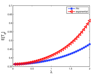
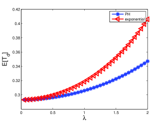
Figure 2: $E\left[T_{d}\right]$s of the PH and exponential distributions for $T(1)$ and $T(2)$, respectively

For $m=3,d=5,\alpha\left(1\right)=\left(1/3,1/3,1/3\right)$ and $\alpha\left(2\right)=\left(1/12,7/12,1/3\right)$,

$$T=\left(\begin{array}[]{ccc}-10&2&4\\ 3&-7&4\\ 0&2&-5\end{array}\right).$$

Table 10 shows how the doubly exponential solution ($\pi_{1}$ to $\pi_{4}$) depends on the vectors $\alpha\left(1\right)$ and $\alpha\left(2\right)$, respectively.

Table 10: The doubly exponential solution depends on the vectors $\alpha$

	$\alpha=(\frac{1}{3},\frac{1}{3},\frac{1}{3})$	$\alpha=(\frac{1}{12},\frac{7}{12},\frac{1}{3})$
$\pi_{1}$	(0.0741, 0.1358 , 0.2346)	(0.0602, 0.1728, 0.2531)
$\pi_{2}$	(5.619e-05, 1.030e-05,  1.779e-04 )	(7.182e-05, 2.063e-04, 3.020e-04)
$\pi_{3}$	(1.411e-20, 2.587e-20, 4.469e-20)	(1.739e-19, 4.993e-19, 7.311e-19)
$\pi_{4}$	(1.410e-98, 2.586e-98, 4.466e-98)	(1.444e-92, 4.148e-92, 6.074e-92)

6 Concluding remarks

In this paper, we provide a matrix-analytic solution for supermarket models. We describe the supermarket model with PH service times as a system of differential vector equations, and provide a doubly exponential solution to the fixed point of the system of differential vector equations. We also provide some numerical examples to illustrate that our approach is effective and efficient in the study of randomized load balancing schemes with non-exponential service requirements, such as, Erlang service time distributions, hyper-exponential service time distributions and PH service time distributions. We expect that this approach will be applicable to study other randomized load balancing schemes, for example, generalizing the arrival process to non-Poisson such as renewal process or Markovian arrival process, generalizing the service times to general probability distributions, and analyzing retrial and processor-sharing service disciplines.

References

[1] Y. Azar, A.Z. Broder, A.R. Karlin and E. Upfal (1999).
Balanced allocations. SIAM Journal on Computing29,
180–200. A preliminary version of this paper appeared in Proceedings of the Twenty-Sixth Annual ACM Symposium on the Theory of
Computing, 1994.
[2] M. Bramson, Y. Lu and B. Prabhakar (2010). Randomized
load balancing with general service time distributions. In Proceedings of the ACM SIGMETRICS international conference on Measurement
and modeling of computer systems, pages 275–286.
[3] M. Dahlin (1999). Interpreting stale load information.
IEEE Transactions on Parallel and Distributed Systems11,
1033 - 1047.
[4] D.L. Eager, E.D. Lazokwska and J. Zahorjan (1986).
Adaptive load sharing in homogeneous distributed systems. IEEE
Transactions on Software Engineering12, 662–675.
[5] D.L. Eager, E.D. Lazokwska and J. Zahorjan (1986). A
comparison of receiver-initiated and sender-initiated adaptive load sharing.
Performance Evaluation Review6, 53–68.
[6] D.L. Eager, E.D. Lazokwska and J. Zahorjan (1988). The
limited performance benefits of migrating active processes for load sharing.
Performance Evaluation Review16, 63–72.
[7] M. Harchol-Balter, A.B. Downey (1997). Exploiting
process lifetime distributions for dynamic load balancing. ACM
Transactions on Computer Systems15, 253–285.
[8] M. Luczak and C. McDiarmid (2006). On the maximum queue
length in the supermarket model. The Annals of Probability34, 493–527.
[9] J.B. Martin (2001). Point processes in fast Jackson
networks. Annals of Applied Probability11, 650-663.
[10] J.B. Martin and Y.M Suhov (1999). Fast Jackson networks.
Annals of Applied Probability9, 854–870.
[11] M.D. Mitzenmacher (1996). Load balancing and density
dependent jump Markov processes. In Proceedings of the
Thirty-Seventh Annual Symposium on Foundations of Computer Science, pages
213–222.
[12] M.D. Mitzenmacher (1996). The power of two choices in
randomized load balancing. PhD thesis, University of California at Berkeley,
Department of Computer Science, Berkeley, CA, 1996.
[13] M. Mitzenmacher (1998). Analyses of load stealing models
using differential equations. In Proceedings of the Tenth ACM
Symposium on Parallel Algorithms and Architectures, pages 212–221.
[14] M. Mitzenmacher (1999). On the analysis of randomized
load balancing schemes. Theory of Computing Systems32,
361–386.
[15] M. Mitzenmacher (1999). Studying balanced allocations
with differential equations. Combinatorics, Probability, and
Computing8, 473–482.
[16] M. Mitzenmacher (2000). How useful is old information?
IEEE Transactions on Parallel and Distributed Systems11,
6–20.
[17] M. Mitzenmacher (2001). The power of two choices in
randomized load balancing. IEEE Transactions on Parallel and
Distributed Computing12, 1094-1104.
[18] M. Mitzenmacher, A. Richa, and R. Sitaraman (2001). The
power of two random choices: a survey of techniques and results. In Handbook of Randomized Computing: volume 1, edited by P. Pardalos, S.
Rajasekaran and J. Rolim, pages 255-312.
[19] M. Mitzenmacher and B. Vöcking (1998). The
asymptotics of selecting the shortest of two, improved. In Proceedings of the 37th Annual Allerton Conference on Communication,
Control, and Computing, pages 326–327. A full version is available as
Harvard Computer Science TR-08-99.
[20] R. Mirchandaney, D. Towsley, and J.A. Stankovic (1989).
Analysis of the effects of delays on load sharing. IEEE Transactions
on Computers38, 1513–1525.
[21] Y.M. Suhov and N.D. Vvedenskaya (2002). Fast Jackson
Networks with Dynamic Routing. Problems of Information Transmission38, 136{153.
[22] M. Telek and A. Heindl (2002). Matching moments for
acyclic discrete and continuous phase-type distributions of second order.
International Journal of Simulation: Systems, Science & Technology3, 47–57.
[23] B. Vöcking (1999). How asymmetry helps load
balancing. In Proceedings of the Fortieth Annual Symposium on
Foundations of Computer Science, pages 131–140.
[24] N.D. Vvedenskaya, R.L. Dobrushin and F.I. Karpelevich.
(1996). Queueing system with selection of the shortest of two queues: An
asymptotic approach. Problems of Information Transmissions32, 20–34.
[25] N.D. Vvedenskaya and Y.M. Suhov (1997). Dobrushin’s
mean-field approximation for a queue with dynamic routing. Markov
Processes and Related Fields3, 493–526.
[26] S. Zhou (1988). A trace-driven simulation study of
dynamic load balancing. IEEE Transactions on Software Engineering14, 1327–1341.