Low-Complexity Detection/Equalization in Large-Dimension MIMO-ISI Channels Using Graphical Models
Abstract
In this paper, we deal with low-complexity near-optimal detection/equalization in large-dimension multiple-input multiple-output inter-symbol interference (MIMO-ISI) channels using message passing on graphical models. A key contribution in the paper is the demonstration that near-optimal performance in MIMO-ISI channels with large dimensions can be achieved at low complexities through simple yet effective simplifications/approximations, although the graphical models that represent MIMO-ISI channels are fully/densely connected (loopy graphs). These include 1) use of Markov Random Field (MRF) based graphical model with pairwise interaction, in conjunction with message/belief damping, and 2) use of Factor Graph (FG) based graphical model with Gaussian approximation of interference (GAI). The per-symbol complexities are and for the MRF and the FG with GAI approaches, respectively, where and denote the number of channel uses per frame, and number of transmit antennas, respectively. These low-complexities are quite attractive for large dimensions, i.e., for large . From a performance perspective, these algorithms are even more interesting in large-dimensions since they achieve increasingly closer to optimum detection performance for increasing . Also, we show that these message passing algorithms can be used in an iterative manner with local neighborhood search algorithms to improve the reliability/performance of -QAM symbol detection.
Index Terms:
MIMO-ISI channels, severe delay spreads, large dimensions, low-complexity detection, graphical models, Markov random fields, pairwise interaction, factor graphs.I Introduction
Signaling in large dimensions can offer attractive benefits in wireless communications. For example, transmission of signals using large spatial dimensions in multiple-input multiple-output (MIMO) systems with large number of transmit/receive antennas can offer increased spectral efficiencies [1]-[3]. The spectral efficiency in a V-BLAST MIMO system is symbols per channel use, where is the number of transmit antennas [3]. Severely delay-spread inter-symbol interference (ISI) channels can offer opportunities to harness rich diversity benefits [4]. In an -length ISI channel, each symbol in a frame is interfered by its previous symbols. However, the availability of copies of the transmitted signal in ISI channels can be exploited to achieve th order diversity. A way to achieve this diversity is to organize data into frames, where each frame consists of channel uses (i.e., dimensions in time), , and carry out joint detection/equalization over the entire frame at the receiver. A MIMO-ISI channel with large and (referred to as large-dimension MIMO-ISI channel) is of interest because of its potential to offer high spectral efficiencies (in large ) and diversity orders (in large 111A practical example of severely delay-spread ISI channel with large is an ultra wideband (UWB) channel [5]. UWB channels are highly frequency-selective, and are characterized by severe ISI due to large delay spreads [6]-[9]. The number of multipath components (MPC) in such channels in indoor/industrial environments has been observed to be of the order of several tens to hundreds; number of MPCs ranging from 12 to 120 are common in UWB channel models [6],[9].). A major challenge, however, is detection complexity. The complexity of optimum detection is exponential in number of dimensions, which is prohibitive for large number of dimensions. Our focus in this paper is to achieve near-optimal detection performance in large dimensions at low complexities. A powerful approach to realize this goal, which we investigate in this paper, is message passing on graphical models.
Graphical models are graphs that indicate inter-dependencies between random variables [10]. Well known graphical models include Bayesian belief networks, factor graphs, and Markov random fields [11]. Belief propagation (BP) is a technique that solves inference problems using graphical models [11]. BP is a simple, yet highly effective, technique that has been successfully employed in a variety of applications including computational biology, statistical signal/image processing, data mining, etc. BP is well suited in several communication problems as well [10]; e.g., decoding of turbo codes and LDPC codes [12],[13], multiuser detection in CDMA [14]-[16], and MIMO detection [17]-[20].
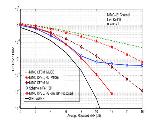
Turbo equalization which performs detection/equalization and decoding in an iterative manner in coded data transmission over ISI channels have been widely studied [21],[22],[23]. More recently, message passing on factor graphs based graphical models [24] have been studied for detection/equalization on ISI channels [25]-[30]. In [27], it has been shown through simulations that application of sum-product (SP) algorithm to factor graphs in ISI channels converges to a good approximation of the exact a posteriori probability (APP) of the transmitted symbols. In [28], the problem of finding the linear minimum mean square error (LMMSE) estimate of the transmitted symbol sequence is addressed employing a factor graph framework. Equalization in MIMO-ISI channels using factor graphs are investigated in [29],[30]. In [29], variable nodes of the factor graph correspond to the transmitted symbols, and each channel use corresponds to a function node. Since the received signal at any channel use depends on the past symbols transmitted from every transmit antenna, every function node is connected to variable nodes. Near-MAP (maximum a posteriori probability) performance was shown through simulations for systems. However, the complexities involved in the computation of messages at the variable and function nodes are exponential in , which are prohibitive for large spatial dimensions and delay spreads. In [30], a Gaussian approximation of interference is used which significantly reduced the complexity to scale well for large . However, in terms of performance, the algorithm in [30] exhibited high error floors222Figure 14 shows an error floor in the approach in [30]. Whereas, in the same figure, our FG approach in Sec. IV is seen to avoid flooring and perform significantly better..
Our key contribution in this paper is the demonstration that graphical models can be effectively used to achieve near-optimal detection/equalization performance in large-dimension MIMO-ISI channels at low complexities. The achieved performance is good because detection is performed jointly over the entire frame of data; i.e., over the full data vector. While simple approximations/simplifications resulted in low complexities, the large-dimension behavior333We say that an algorithm exhibits ‘large-dimension behavior’ if its bit error performance improves with increasing number of dimensions. The fact that turbo codes with BP decoding achieve near-capacity performance only when the frame sizes are large is an instance of large-dimension behavior. natural in message passing algorithms contributed to the near-optimal performance in large dimensions. The graphical models we consider in this paper are Markov random fields (MRF) and factor graphs (FG). We show that these graphical models based algorithms perform increasingly closer to the optimum performance for increasing and increasing values of and , keeping fixed.
In the case of MRF approach (Section III), we show that the use of damping of messages/beliefs, where messages/beliefs are computed as a weighted average of the message/belief in the previous iteration and the current iteration (details and associated references given in Section III-D), is instrumental in achieving good performance. Simulation results show that the MRF approach exhibits large-dimension behavior, and that damping significantly improves the bit error performance (details given in Section III-F). For example, the MRF based algorithm with message damping achieves close to unfaded single-input single-output (SISO) AWGN performance (which is a lower bound on the optimum detector performance) within 0.25 dB at bit error rate (BER) in a MIMO-ISI channel with , channel uses per frame (i.e., problem size is dimensions), and equal-energy multipath components (MPC). Similar performances are shown for large-MIMO systems with and (problem size and 2048 dimensions). The per-symbol complexity of the MRF approach is (details in Section III-E).
In the case of FG approach (Section IV), the Gaussian approximation of interference (GAI) we adopt is found to be effective to further reduce the complexity by an order (Section IV-A); i.e., the per-symbol complexity of the FG with GAI approach is just , which is one order less than that of the MRF approach. The proposed FG with GAI approach is also shown to exhibit large-dimension behavior; its BER performance is almost the same as that of the MRF approach, and is significantly better than that of the scheme in [30] (Section IV-B). We also show that the proposed FG with GAI algorithm can be used in an iterative manner with local neighborhood search algorithms, like the reactive tabu search (RTS) algorithm in [34], to improve the performance of -QAM detection (Section V).
Though the proposed algorithms are presented in the context of uncoded systems, they can be extended to coded systems as well, through turbo equalization [21]-[23] (Receiver C in Fig. 1 of [23]) or through joint processing of the entire coded frame using low-complexity graphical models (low-complexity approximations of Receiver A in Fig. 1 of [23]). In [19], we have investigated a scheme with separate MRF based detection followed by decoding (Receiver B is Fig. 1 of [23]) in a large-MIMO system, and showed that a coded BER performance close to within 2.5 dB of the theoretical ergodic MIMO capacity is achieved. MIMO space-time coding schemes that can achieve separability of detection and decoding without loss of optimality [43] are interesting because they avoid the need for joint processing for optimal detection and decoding. If such detection-decoding separable space-time codes become available for large dimensions, the proposed algorithms can be applicable in their detection/equalization.
The rest of the paper is organized as follows. In Section II, we present the considered MIMO system model in frequency selective fading. In Section III, we present the proposed MRF based BP detector with damping and its BER performance in large dimensions. Section IV presents the FG with GAI based BP detector and its BER performance. In Section V, the proposed hybrid RTS-BP algorithm for detection of -QAM signals and its performance are presented. Conclusions are presented in Section VI.
II System Model
We consider MIMO systems with cyclic prefixed single-carrier (CPSC) signaling, where the overall MIMO channel includes an FFT operation so that the transmitted symbols are estimated from the received frequency-domain signal (also referred to as SC-FDE: single-carrier modulation with frequency-domain equalization) [44]-[46]. Unlike OFDM signaling, CPSC signaling does not suffer from the peak to average power ratio (PAPR) problem. Also, CPSC with FD-MMSE equalizer performs better than OFDM at large frame sizes (large ) [46]. We will see that our proposed BP based algorithms scale well for large dimensions in MIMO-CPSC schemes (large ) and perform significantly better than MIMO-CPSC with FD-MMSE equalizer as well as MIMO-OFDM with MMSE/ML equalizer.
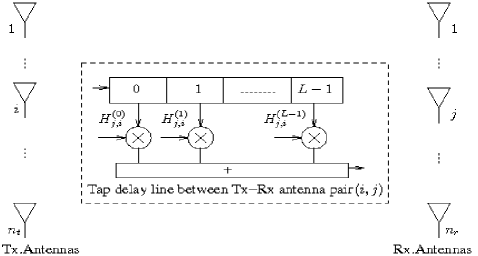
Consider a frequency-selective MIMO channel with transmit and receive antennas as shown in Fig. 1. Let denote the number of multipath components (MPC). Data is transmitted in frames, where each frame has channel uses, out of which data symbol vectors are sent in channel uses . These channel uses are preceded by a cyclic prefix (CP) of length channel uses so that . In each channel use, an -length data symbol vector is transmitted using spatial multiplexing on transmit antennas. Let denote the data symbol vector transmitted in the th channel use, . Though the symbol alphabet used here is BPSK, extensions to higher-order alphabet are possible, and some are discussed later in the paper. While CP avoids inter-frame interference, there will be ISI within the frame. The received signal vector at time can be written as
| (1) |
where , is the channel gain matrix for the th MPC such that denotes the entry on the th row and th column of the matrix, i.e., is the channel from th transmit antenna to the th receive antenna on the th MPC. The entries of are assumed to be i.i.d . It is further assumed that , remain constant for one frame duration, and vary i.i.d from one frame to the other. is the additive white Gaussian noise vector at time , whose entries are independent, each with variance , where is the average received SNR per received antenna. The CP will render the linearly convolving channel to a circularly convolving one, and so the channel will be multiplicative in frequency domain. Because of the CP, the received signal in frequency domain, for the th frequency index (), can be written as
| (2) |
where , and . Stacking the vectors , , we write
| (3) |
where
where , is the -point DFT matrix and denotes the Kronecker product. Equation (3) can be written in an equivalent linear vector channel model of the form
| (5) |
where , , and . Note that the well known MIMO system model for flat fading can be obtained as a special case in the above system model with .
We further note that, in the considered system, signaling is done along dimensions in time and dimensions in space, so that the total number of dimensions involved is . We are interested in low-complexity detection/equalization in large dimensions (i.e., for large ) using graphical models. The goal is to obtain an estimate of vector , given and the knowledge of . The optimal maximum a posteriori probability (MAP) detector takes the joint posterior distribution
| (6) |
and marginalizes out each variable as , where stands for all entries of except . The MAP estimate of the bit , , is then given by
| (7) |
whose complexity is exponential in . In the following sections, we present low-complexity detection algorithms based on graphical models suited for the system model in (5) with large dimensions, i.e., for large , , , keeping fixed.
III Detection Using BP on Markov Random Fields
In this section, we present a detection algorithm based on message passing on a MRF graphical model of the MIMO system model in (5) [31].
III-A Markov Random Fields
An undirected graph is given by , where is the set of nodes and is the set of undirected edges. An MRF is an undirected graph whose vertices are random variables [35],[10]. The statistical dependency among the variables are such that any variable is independent of all the other variables, given its neighbors. Usually, the variables in an MRF are constrained by a compatibility function, also known as a clique potential in literature. A clique of an MRF is a fully connected sub-graph, i.e., it is a subset such that for all . A clique is maximal if it is not a strict subset of another clique. Therefore, a maximal clique does not remain fully connected if any additional vertex of the MRF is included in it. For example, in the MRF shown in Fig. 2, and are two maximal cliques.

Let there be maximal cliques in the MRF, and be the variables in maximal clique . Let be the clique potential of clique . Then the joint distribution of the variables is given by Hammersley-Clifford theorem [47]
| (8) |
where is a constant, also known as partition function, chosen to ensure the distribution is normalized. In Fig. 2, with two maximal cliques in the MRF, namely, and , the joint probability distribution is given by
| (9) |
Pairwise MRF: An MRF is called a pairwise MRF if all the maximal cliques in the MRF are of size two. In this case, the clique potentials are all functions of two variables. The joint distribution in such a case takes the form [11]
| (10) |
where is the clique potential between nodes and denoting the statistical dependence between them, and is the self potential of node .
III-B MRF of MIMO System
The MRF of a MIMO system is a fully connected graph. Figure 3 shows the MRF for a MIMO system. We get the MRF potentials for the MIMO system where the posterior probability function of the random vector , given and , is of the form444In our detection problem, relative values of the distribution for various possibilities of are adequate. So, we can omit the normalization constant , which is independent of , and replace the equality with proportionality in the distribution.
| (11) | |||||
Now, defining and , we can write (11) as
| (12) | |||||
where and are the elements of and , respectively. Comparing (12) and (10), we see that the MRF of the MIMO system has only pairwise interactions with the following potentials
| (13) | |||||
| (14) |

III-C Message Passing
The values of and given by (13) and (14) define, respectively, the edge and self potentials of an undirected graphical model to which message passing algorithms, such as belief propagation (BP), can be applied to compute the marginal probabilities of the variables. BP attempts to estimate the marginal probabilities of all the variables by way of passing messages between the local nodes.
A message from node to node is denoted as , and belief at node is denoted as , . The is proportional to how likely was transmitted. On the other hand, is proportional to how likely thinks was transmitted. The belief at node is
| (15) |
where denotes the neighboring nodes of node , and the messages are defined as [11]
| (16) |
Equation (16) actually constitutes an iteration, as the message is defined in terms of the other messages. So, BP essentially involves computing the outgoing messages from a node to each of its neighbors using the local joint compatibility function and the incoming messages and transmitting them. The algorithm terminates after a fixed number of iterations.
III-D Improvement through Damping
In systems characterized by fully/highly connected graphical models, BP based algorithms may fail to converge, and if they do converge, the estimated marginals may be far from exact [36],[37]. It may be expected that BP might perform poorly in MIMO graphs due to the high density of connections. However, several methods are known in the literature, including double loop methods [38],[39] and damping [40],[41] which can be applied to improve things if BP does not converge (or converges too slowly). In this paper, we consider damping methods.
In [40], Pretti proposed a modified version of BP with over-relaxed BP dynamics. At each step of the algorithm, the evaluation of messages is taken to be a weighted average between the old estimate and the new estimate. The weighted average could either be applied to the messages (resulting in message damped BP) or to the estimate of the probability distribution/beliefs of the variables (probability/belief damped BP), or to both messages and beliefs (hybrid damped BP). It is shown, in [40], that the probability damped BP can be derived as a limit case in which the double-loop algorithm becomes a single-loop one.
Message Damped BP: Denoting as the updated message in iteration obtained by message passing, the new message from node to node in iteration , denoted by , is computed as a convex combination of the old message and the updated message as
| (17) |
| (18) |
where is referred as the message damping factor.
Belief Damping: Instead of damping the messages in each iteration, the beliefs of the variables can be computed in each iteration as a weighted average, as
| (19) |
| (20) |
where is referred to as the belief damping factor.
Hybrid Damping: As a more general damping strategy, we can update both the messages as well as the beliefs according to (18) and (20), respectively, in each iteration. Different combinations of values specializes to different strategies; for e.g., corresponds to Undamped BP, corresponds to Message damped BP, corresponds to Belief damped BP, and corresponds to Hybrid damped BP.
The proposed BP algorithm employing damping is listed in Table I.
III-E Computation Complexity
The per-symbol complexity of calculating messages and beliefs in a single BP iteration is and , respectively. Likewise, the per-symbol complexity of computing and is and , respectively. The computation of can be carried out with per-symbol complexity. The computation of involves computation of , which involves three operations: computation of , calculation of , and multiplication of and with . The computation involves -point FFT of matrices , , each of dimension . The complexity associated with this operation is . The total number of symbols transmitted is . So, the per-symbol complexity is . The computation involves the calculation of for . The computation of each has complexity . Due to block-diagonal structure of , such computations can be done in complexity, leading to a per-symbol complexity of . Likewise, due to the block-symmetric structure of , the per-symbol complexity corresponding to computation is . Since the number of BP iterations is much less than , the overall per-symbol complexity is of the proposed MRF based BP detection algorithm is given by , which scales well for large .
| Initialization |
| 1. , |
| , |
| 2. , |
| 3. ; |
| 4. for = 1 to |
| 5. |
| 6. end for |
| 7. for = 1 to |
| 8. for = 1 to , |
| 9. |
| 10. end for |
| 11. end for |
| Iterative Update of Messages and Beliefs |
| 12. for = 1 to |
| Damped Message Calculation |
| 13. for = 1 to |
| 14. for = 1 to |
| 15. |
| 16. |
| 17. end for |
| 18. end for |
| Damped Belief Calculation |
| 19. for = 1 to |
| 20. |
| 21. |
| 22. end for |
| 23. end for; End of for loop starting at line 12 |
| 24. |
| 25. Terminate |
III-F Simulation Results
In this section, we present the simulated BER performance of the proposed MRF BP detection algorithm.
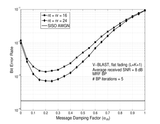
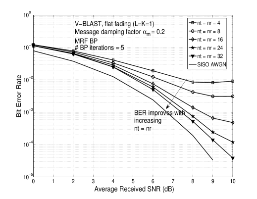
Performance in Flat-Fading with Large : In Figs. 4 to 6, we illustrate the ‘large-dimension behavior’ of the algorithm and the effect of damping for large number (tens) of transmit and receive antennas with BPSK modulation on flat fading channels (i.e., ). The number of BP iterations is 5. Figure 4 shows the variation of the achieved BER as a function of the message damping factor, , in and V-BLAST MIMO systems at an average received SNR per receive antenna, , of 8 dB. Note that corresponds to the case of undamped BP. It can be observed from Fig. 4 that, depending on the choice of the value of , message damping can significantly improve the BER performance of the BP algorithm. There is an optimum value of at which the BER improvement over no damping case is maximum. For the chosen set of system parameters in Fig. 4, the optimum value of is observed to be about 0.2. For this optimum value of , it is observed that about an order of BER improvement is achieved with message damping compared to that without damping. From Fig. 4, it can further be seen that the performance improves for increasing (i.e., performance of the system is better that of the system). This shows that the algorithm exhibits ‘large-dimension behavior,’ where the BER performance moves closer towards unfaded SISO AWGN performance when is increased from 16 to 24. This large-dimension behavior is illustrated even more clearly in Fig. 5, where we plot the BER performance of V-BLAST MIMO as a function of SNR for different and for .
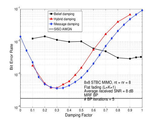
In Fig. 6, we present a comparison of the BER performance achieved using message damping, belief damping and hybrid damping based BP detection of non-orthogonal space-time block code (STBC) from cyclic division algebra (CDA) with , [42] at 8 dB SNR. In this type of STBC, each STBC is a square matrix with transmit antennas and time slots constructed using symbols, which results in dimensions and symbols per channel use. For message damping and belief damping, and are varied in the range 0 to 1. For hybrid damping, we set and varied it in the range 0 to 1. From Fig. 6, it can be seen that with damping, there is an optimum value of the damping factor at which the BER performance is the best (e.g., for message damping, the optimum damping factor is about 0.3 in Fig. 6), message damping performs better than belief damping for small values of the damping factor, whereas belief damping performs better at high values of the damping factor; however, over the entire range of the damping factor, the best performance of message damping is significantly better than the best performance of belief damping, and for the chosen condition of , hybrid damping performance is similar to that of message damping; however, and in hybrid damping can be jointly optimized to further improve the performance.
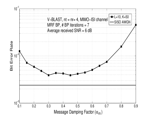
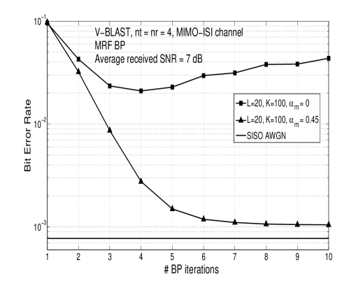
Performance in MIMO-ISI Channels with Large : In Fig. 7, we explore the effect of message damping on the BER performance of the MRF based BP detector/equalizer in MIMO-ISI channels. In all the simulations of MIMO-ISI channels, we have taken uniform power delay profile (i.e., all the paths are assumed to have equal energy). Figure 7 shows the variation of the achieved BER as a function of the message damping factor, , for , BPSK, , at an average received SNR of 6 dB. The total number of dimensions, . The number of BP iterations used is 7. From Fig. 7, it is can be seen that damping can significantly improve the BER performance of the BP algorithm. For the chosen set of system parameters in Fig. 7, the optimum value of is observed to be about 0.45, which gives about an order of BER improvement. This point of the benefit of damping in terms of BER performance (and also in terms of convergence) is even more clearly brought out in Fig. 8, where we have compared the BER performance without damping () and with damping () for at an SNR of 7 dB as a function of the number of BP iterations. It is interesting to see that without damping (i.e., with ), the algorithm indeed shows ‘divergence’ behavior, i.e., BER increases as number of iterations is increased beyond 4. Such divergence behavior is effectively removed by damping, as can be seen from the BER performance achieved with . Indeed the algorithm with damping () is seen to be converge smoothly. It is also interesting to note that the algorithm converges to a BER which is quite close to the unfaded SISO AWGN BER (BER on SISO AWGN at 7 dB SNR is about and the converged BER using damped BP is about ). This illustrates the potential of damping in improving BER performance and convergence of the algorithm when employed for detection/equalization in the considered MIMO system on severely delay spread frequency-selective channels (e.g., ). It is also noted that damping (as per Eqn. (18)) does not increase the order of complexity of the algorithm without damping; the order of complexity without and with damping remains the same.
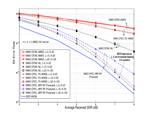
Comparison with MIMO-OFDM Performance: In Fig. 9, we present a performance comparison between the considered MIMO-CPSC scheme and a MIMO-OFDM scheme for the same system/channel parameters in both cases; for and following combinations of and : , , . For MIMO-CPSC, two detection schemes are considered: FD-MMSE and proposed MRF BP. For the MRF BP, number of BP iterations used is 10 and the value of used is 0.45. For MIMO-OFDM, two detection schemes, namely, MMSE and ML detection on each subcarrier are considered. We have also plotted the unfaded SISO AWGN performance that serves as a lower bound on the optimum detection performance. The following observations can be made from Fig. 9: MIMO-OFDM with MMSE detection performs the worst among all the considered system/detection configurations, MIMO-CPSC with FD-MMSE performs better than MIMO-OFDM with MMSE (this better performance in CPSC is in line with other reported comparisons between OFDM and CPSC, e.g., [44],[45],[46]), at the expense of increased detection complexity, MIMO-OFDM with ML detection performs better than both MIMO-OFDM with MMSE and MIMO-CPSC with FD-MMSE, and more interestingly, MIMO-CPSC with the low-complexity MRF BP detection significantly outperforms MIMO-OFDM even with ML detection. Indeed, the performance of the MIMO-CPSC with MRF BP detection gets increasingly closer to the SISO AGWN performance for increasing , , keeping constant. For example, the gap between the MRF BP performance and the SISO AWGN performance is only about 0.25 dB for at a BER of . This illustrates the ability of the MRF BP algorithm to achieve near-optimal performance for severely delay spread MIMO-ISI channels (i.e., large ) as witnessed in UWB systems.
IV Detection using BP on Factor Graphs with Gaussian Approximation of Interference
In this section, we present another low-complexity algorithm based on BP for detection in large-dimension MIMO-ISI channels. The graphical model employed here is factor graphs. A key idea in the proposed factor graph approach which enables to achieve low-complexity is the Gaussian approximation of interference (GAI) in the system.


Consider the MIMO system model in (5). We will treat each entry of the observation vector as a function node (observation node) in a factor graph, and each transmitted symbol as a variable node. The received signal can be written as
| (21) | |||||
When computing the message from the th observation node to the th variable node, we make the following Gaussian approximation of the interference:
| (22) |
where the interference plus noise term, , is modeled as with
| (23) |
| (24) |
For BPSK signaling, the log-likelihood ratio (LLR) of the symbol at observation node , denoted by , can be written as
| (25) | |||||
The LLR values computed at the observation nodes are passed to the variable nodes (Fig. 10a). Using these LLRs, the variable nodes compute the probabilities
| (26) | |||||
and pass them back to the observation nodes (Fig. 10b). This message passing is carried out for a certain number of iterations. Messages can be damped as described in Section III-D and then passed. Finally, is detected as
| (27) |
Note that approximating the interference as Gaussian greatly simplifies the computation of messages (as can be seen from the complexity discussion in the following subsection.)
IV-A Computation Complexity
The computation complexity of the FG-GAI BP algorithm in the above involves LLR calculations at the observation nodes as per (25), which has complexity, and calculation of probabilities at variable nodes as per (26), which also requires complexity555A naive implementation of (25) would require a summation over variable nodes for each message, amounting to a complexity of order . However, the summation over variables in (23) can be written in the form , where the computation of the full summation from to (which is independent of the variable index ) requires additions. In addition, one subtraction operation for each is required. The makes the complexity order for computing (23) to be only . A similar argument holds for computation of the variance in (24), and hence the complexity of computing the LLR in (25) becomes . Likewise, a similar rewriting of the summation in (26) leads to a complexity of .. Hence, the overall complexity of the algorithm is for detecting transmitted symbols. So the per-symbol complexity is just for . Note that this complexity is one order less than that of the MRF based approach in the previous section. Because of its linear complexity in and , the proposed FG approach with GAI is quite attractive for detection in large-dimension MIMO-ISI channels. In addition, the BER performance achieved by the algorithm in large dimensions is very good (as shown in the BER performance results in the following subsection).
IV-B Simulation Results
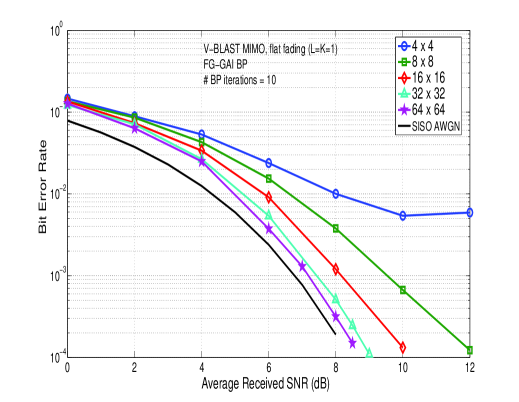
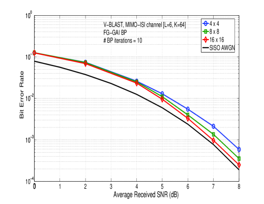
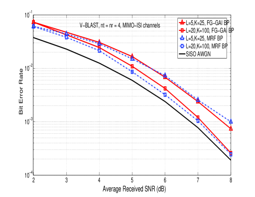
Figure 11 shows the simulated BER performance of the FG-GAI BP algorithm in V-BLAST MIMO with and BPSK on flat fading (). The number of BP iterations and and message damping factor used are 10 and 0.4, respectively. We observe that, like the MRF approach, the FG-GAI approach also exhibits large-dimension behavior; e.g., and V-BLAST systems perform close to unfaded SISO AWGN performance. Similar large-dimension behavior is shown in Fig. 12 in MIMO-ISI channels with and for ; i.e., BERs move increasingly closer to unfaded SISO AWGN BER for increasing . Figure 13 presents a comparison of the performances achieved by the MRF and FG-GAI approaches for the following system settings: , , , and BPSK. It can be seen that, for these system settings, the FG with GAI approach performs almost the same as the MRF approach, at one order lesser complexity than that of the MRF approach.
Figure 14 presents a comparison of the performances achieved by the proposed scheme and the scheme in [30] for , , and BPSK. It can be seen that while the scheme in [30] exhibits an error floor, the proposed scheme avoids flooring and achieves much better performance. Such good performance is achieved because equalization is done jointly on all the symbols in a frame. The complexity of the scheme in [30] is , whereas the complexity of the proposed scheme is . Though , the linear complexity of the proposed scheme in is still very attractive. Also, as with MRF BP, the FG-GAI BP algorithm in MIMO-CPSC performs significantly better than MIMO-OFDM even with ML detection.
V Hybrid Algorithms Using BP and Local Neighborhood Search for -QAM
The BP algorithms proposed in the previous two sections are for BPSK modulation, i.e., for . They can work for 4-QAM also by viewing the transmit symbol vector to be in . Low-complexity algorithms for detection/equalization for higher-order -QAM, , over large dimension MIMO-ISI channels are of interest. A BP based algorithm that is suited for higher-order QAM in MIMO has been reported recently in [49]. The algorithm in [49] uses a Gaussian tree approximation (GTA) to convert the fully-connected graph representing the MIMO system into a tree, and carries out BP on the resultant approximate tree. We refer to this algorithm in [49] as the GTA BP algorithm. In this section, we take an alternate hybrid approach for efficient detection of -QAM signals, where the proposed FG-GAI BP algorithm for BPSK is used to improve the -QAM detection performance of local neighborhood search algorithms. Simulation results (Fig. 17) show that the proposed hybrid approach performs better than the GTA BP approach in [49].
Local Neighborhood Search Based Detection: Low complexity search algorithms that attempt to minimize the maximum-likelihood (ML) cost , by limiting the search space to local neighborhood have been proposed for detection of -QAM signals in MIMO – e.g., tabu search (TS) algorithm [32]-[34]. Such local neighborhood search algorithms have the advantage of low-complexity (e.g., TS algorithms, like the proposed MRF BP algorithm, has quadratic complexity in ), making them suited for large dimensions. However, their higher-order QAM performance is away from optimal performance. Here, we propose to improve the -QAM performance of these search algorithms through the application of the proposed BP algorithms on the search algorithm outputs. This approach essentially improves the reliability of the output symbols from the local neighborhood search, thereby improving the overall BER performance. We apply this hybrid approach to the reactive tabu search (RTS) algorithm in [34].
Hybrid RTS-BP Approach: In the following subsections, we first present a brief summary of the RTS algorithm in [34] and the motivation behind the proposed hybrid approach. Next, we present the proposed hybrid RTS-BP algorithm and its BER performance. Finally, we present a method to reduce complexity based on the knowledge of the simulated pdf of the RTS algorithm output.
V-A Reactive Tabu Search (RTS) Algorithm
Here, we present a brief summary of the RTS algorithm in [34]. The RTS algorithm starts with an initial solution vector, defines a neighborhood around it (i.e., defines a set of neighboring vectors based on a neighborhood criteria), and moves to the best vector among the neighboring vectors (even if the best neighboring vector is worse, in terms of ML cost , than the current solution vector); this allows the algorithm to escape from local minima. This process is continued for a certain number of iterations, after which the algorithm is terminated and the best among the solution vectors in all the iterations is declared as the final solution vector. In defining the neighborhood of the solution vector in a given iteration, the algorithm attempts to avoid cycling by making the moves to solution vectors of the past few iterations as ‘tabu’ (i.e., prohibits these moves), which ensures efficient search of the solution space. The number of these past iterations is parametrized as the ‘tabu period,’ which is dynamically changed depending on the number of repetitions of the solution vectors that are observed in the search path (e.g., increase the tabu period if more repetitions are observed). The per-symbol complexity of the RTS algorithm is quadratic in for .
V-B Motivation for Hybrid RTS-BP Algorithm
The proposed hybrid RTS-BP approach is motivated by the following two observations we made in our BER simulations of the RTS algorithm: the RTS algorithm performed very close to optimum performance in large dimensions for 4-QAM; however, its higher-order QAM performance is far from optimal, and at moderate to high SNRs, when an RTS output vector is in error, the least significant bits (LSB) of the data symbols are more likely to be in error than other bits. An analytical reasoning for the second observation can be given as follows.
Let the transmitted symbols take values from -QAM alphabet , so that is the transmitted vector. Consider the real-valued system model corresponding to (5), given by , where
| (32) |
| (37) |
is a vector; can be viewed to be from an underlying -PAM signal set, and so is . Let denote the -PAM alphabet that takes its value from.
Let denote the detected output vector from the RTS algorithm corresponding to the transmitted vector . Consider the expansion of the -PAM symbols in terms of ’s, where we can write the value of each entry of as a linear combination of ’s as
| (38) |
where and . We note that the RTS algorithm outputs a local minima as the solution vector. So, , being a local minima, satisfies the following conditions:
| (39) |
where , and denotes the th column of the identity matrix. Defining and denoting the th column of as , the conditions in (39) reduce to
| (40) |
where denotes the th element of . Under moderate to high SNR conditions, ignoring the noise, (40) can be further reduced to
| (41) |
where denotes the th column of . For Rayleigh fading, is chi-square distributed with degrees of freedom with mean . Approximating the distribution of to be normal with mean zero and variance for by central limit theorem, we can drop the in (41). Using the fact that the minimum value of is 2, (41) can be simplified as
| (42) |
where . Also, if , by the normal approximation in the above
| (43) |
Now, the LHS in (42) being normal with variance proportional to and the RHS being positive, it can be seen that , take smaller values with higher probability. Hence, the symbols of are nearest Euclidean neighbors of their corresponding symbols of the transmitted vector with high probability666Because ’s and ’s take values from -PAM alphabet, is said to be the Euclidean nearest neighbor of if .. Now, because of the symbol-to-bit mapping in (38), will differ from its nearest Euclidean neighbors certainly in the LSB position, and may or may not differ in other bit positions. Consequently, the LSBs of the symbols in the RTS output are least reliable.
The above observation then led us to consider improving the reliability of the LSBs of the RTS output using the proposed FG-GAI BP algorithm presented in Section IV, and iterate between RTS and FG-GAI BP as follows.

V-C Proposed Hybrid RTS-BP Algorithm
Figure 15 shows the block schematic of the proposed hybrid RTS-BP algorithm. The following four steps constitute the proposed algorithm.
-
•
Step 1: Obtain using the RTS algorithm. Obtain the output bits , , , from and (38).
-
•
Step 2: Using the ’s from Step 1, reconstruct the interference from all bits other than the LSBs (i.e., interference from all bits other than ’s) as
(44) where . Cancel the reconstructed interference in (44) from r as
(45) -
•
Step 3: Run the FG-GAI BP algorithm in Section IV on the vector in Step 2, and obtain an estimate of the LSBs. Denote this LSB output vector from FG-GAI BP as . Now, using from the BP output, and the , from the RTS output in Step 1, reconstruct the symbol vector as
(46) -
•
Step 4: Repeat Steps 1 to 3 using as the initial vector to the RTS algorithm.
The algorithm is stopped after a certain number of iterations between RTS and BP. Our simulations showed that two iterations between RTS and BP are adequate to achieve good improvement; more than two iterations resulted in only marginal improvement for the system parameters considered in the simulations. Since the complexity of BP part of RTS-BP is less than that of the RTS part, the order of complexity of RTS-BP is same as that of RTS, .
V-D Simulation Results
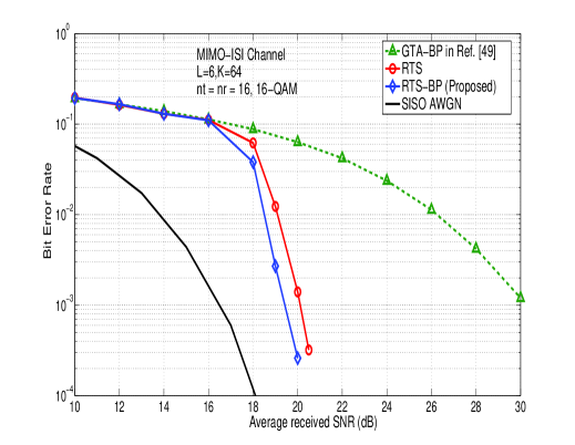
Figure 16 shows the BER performance of the proposed hybrid RTS-BP algorithm in comparison with those of the RTS algorithm and the GTA-BP algorithm in [49] in V-BLAST MIMO with 16-QAM on a frequency selective channel with equal energy multipath components and data vectors per frame. Because of the improvement of the reliability of LSBs due to BP run on them, the RTS-BP algorithm achieves better performance compared to RTS algorithm without BP. Also, both RTS-BP and RTS algorithms perform better than the GTA-BP in [49].
V-E Complexity Reduction Using Selective BP
In the proposed RTS-BP algorithm, the use of BP at the RTS output was done unconditionally. Whereas the use of BP can improve performance only when the RTS output is erroneous. So, the additional complexity due to BP can be avoided if BP is not carried out whenever the RTS output is error-free. To decide whether to use BP or not, we can use the knowledge of the simulated pdf of the ML cost of the RTS output vector, i.e., the pdf of . Figure 17 shows the simulated pdf of for a V-BLAST MIMO system with 64-QAM at an SNR of 30 dB on flat fading (). From Fig. 17, it is seen that a comparison of the value of with a suitable threshold can give an indication of the reliability of the RTS output. For example, the output is more likely to be erroneous if in Fig. 17.
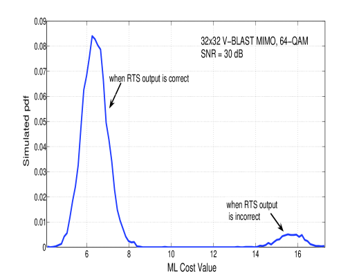
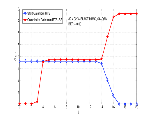
Based on the above observation, we modify the RTS-BP algorithm as follows. If , only then BP algorithm is used; otherwise, the RTS output is taken as the final output. The threshold has to be carefully chosen to achieve good performance. It is seen that corresponds to the case of unconditional RTS-BP, and corresponds to the case of RTS without BP. For , there is no additional complexity due to BP, but there is no performance gain compared to RTS. For , performance gain is possible compared to RTS, but BP complexity will be there for all realizations. So there exits a performance-complexity trade off as a function of . We illustrate this trade-off in Fig. 18 for a V-BLAST system with 64-QAM in flat fading. For this purpose, we define ‘SNR gain’ in dB for a given threshold as the improvement in SNR achieved by RTS with selective BP using threshold to achieve an uncoded BER of compared to RTS without BP. Likewise, we define ‘complexity gain’ for a given as , where is the ratio of the average number of computations required to achieve uncoded BER in unconditional RTS-BP and that in RTS with selective BP using threshold . In Fig. 18, we plot these two gains on the y-axis as a function of the threshold . From this figure, we can observe that for values less than 4, there is not much complexity gain since such small threshold values invoke BP more often (i.e., the system behaves more like unconditional RTS-BP). Similarly, for values greater than 14, the system behaves more like RTS without BP; i.e., the complexity gain is maximum but there is no SNR gain. Interestingly, for values in the range 4 to 14, maximum SNR gain is retained while achieving significant complexity gain as well.
VI Conclusions
In this paper, we demonstrated that belief propagation on graphical models including Markov random fields and factor graphs can be efficiently used to achieve near-optimal detection in large-dimension MIMO-ISI channels at quadratic and linear complexities in . It was shown through simulations that damping of messages/beliefs in the MRF BP algorithm can significantly improve the BER performance and convergence behavior. The Gaussian approximation of interference we adopted in the factor graph approach is novel, which offered the attractive linear complexity in number of dimensions while achieving near-optimal performance in large dimensions. In higher-order QAM, iterations between a tabu search algorithm and the proposed FG-GAI BP algorithm was shown to improve the bit error performance of the basic tabu search algorithm. Although we have demonstrated the proposed algorithms in uncoded systems, they can be extended to coded systems as well, using either turbo equalization or joint processing of the entire coded symbol frame based on low-complexity graphical models. Finally, a theoretical analysis of the convergence behavior and the bit error performance of the proposed BP algorithms is challenging, and remains to be studied.
References
- [1] G. J. Foschini and M. J. Gans, “On limits of wireless communications in a fading environment when using multiple antennas,” Wireless Pers. Commun., vol. 6, pp. 311-335, March 1998.
- [2] I. E. Telatar, “Capacity of multi-antenna Gaussian channels,” European Trans. on Telecommun., vol. 10, no. 6, pp. 585-595, November 1999.
- [3] A. Paulraj, R. Nabar, and D. Gore, Introduction to Space-Time Wireless Communications, Cambridge University Press, 2003.
- [4] J. G. Proakis, Digital Communications, 4th Ed., Mc-Graw Hill, 2001.
- [5] X. Shen, M. Guizani, R. C. Qiu, and T. Le-Ngoc, Ultra-wideband Wireless Communications and Networks, John Wiley & Sons, 2006.
- [6] A. F. Molisch, J. R. Foerster, M. Pendergrass, “Channel models for ultrawideband personal area networks,” IEEE Wireless Commun., vol. 10, no. 6, pp. 14–21, December 2003.
- [7] A. F. Molisch, “Ultrawideband propagation channels - Theory, measurement, and modeling,” IEEE Trans. on Veh. Tech., vol. 54, no. 5, pp. 1528-1545, September 2005.
- [8] J. Karedal, S. Wyne, P. Almers, F. Tufvesson, and A. F. Molisch, “Statistical analysis of the UWB channel in an industrial environment,” Proc. IEEE VTC’2004-Fall,, pp. 81-85, September 2004.
- [9] R. Saadane and A. M. Hayar, “DRB1.3 third report on UWB channel models,” http://www.eurecom.fr/util/publidownload.fr.htm?id=2112, Newcom, November 2006.
- [10] B. J. Frey, Graphical Models for Machine Learning and Digital Communication, Cambridge: MIT Press, 1998.
- [11] J. S. Yedidia, W. T. Freeman, Y. Weiss, “Understanding belief propagation and its generalizations,” MERL Tech. Rep. TR-2001-22, January 2002.
- [12] R. J. McEliece and D. J. C. MacKay, and J-F. Cheng, “Turbo decoding as an instance of Pearl’s belief propagation algorithm,” IEEE Jl. Sel. Areas in Commun., vol. 16, no.2, pp. 140-152, February 1998.
- [13] D. J. C. MacKay, “Good error-correcting codes based on very sparse matrices,” IEEE Trans. on Inform. Theory, vol. 45, no. 2, pp. 399-431, March 1999.
- [14] Y. Kabashima, “A CDMA multiuser detection algorithm on the basis of belief propagation,” Journal of Physics A: Mathematical and General, pp. 11111-11121, October 2003.
- [15] A. Montanari, B. Prabhakar, and D. Tse, “Belief propagation based multiuser detection,” Online arXiv:cs/0510044v2 [cs.IT] 22 May 2006.
- [16] D. Guo and C-C. Wang, “Multiuser detection of sparsely spread CDMA,” IEEE JSAC Spl. Iss. on Multiuser Detection, for Adv. Commun. Systems and Networks, vol. 26, no. 3, pp. 421-431, April 2008.
- [17] J. Soler-Garrido, R. J. Piechocki, K. Maharatna, and D. McNamara, “Analog MIMO detection on the basis of belief propagation,” Proc. IEEE Mid-West Symp. on Circuits and Systems, 2006.
- [18] X. Yang, Y. Xiong, F. Wang, “An adaptive MIMO system based on unified belief propagation detection,” Proc. IEEE ICC’2007, June 2007.
- [19] Madhekar Suneel, Pritam Som, A. Chockalingam, and B. Sundar Rajan, “Belief propagation based decoding of large non-orthogonal STBCs,” Proc. IEEE ISIT’2009, Seoul, July 2009.
- [20] P. Som, T. Datta, A. Chockalingam, and B. S. Rajan, “Improved large-MIMO detection based on damped belief propagation,” Proc. IEEE Inform. Theory Workshop (ITW’2010), Cairo, January 2010.
- [21] C. Douillard, M. Jezequel, and C. Berrou, “Iterative correction of intersymbol interference: Turbo equalization,” European Trans. on Telecommunications, vol. 6, pp. 507-511, September-October 1995.
- [22] M. Tuchler, R. Koetter, and A. C. Singer, “Turbo Equalization: Principles and New Results,” IEEE Trans. on Commun., vol. 50, no. 5, pp. 754-767, May 2002.
- [23] R. Koetter, A. C. Singer, and M. Tuchler, “Turbo equalization,” IEEE Sig. Process. Mag., pp. 67-80, January 2004.
- [24] F. R. Kschischang, B. J. Frey, and H.-A. Loeliger, “Factor graphs and the sum-product algorithm,” IEEE Trans. on Inform. Theory, vol. 47, no. 2, pp. 498-519, February 2001
- [25] M. Tutchler, R. Koetter, and A. C. Singer, “Graphical models for coded data transmission over inter-symbol interference channels,” European Trans. on Telecommunications, vol. 5, no. 4, July/August 2004.
- [26] O. Shental, A. J. Weiss, N. Shental, and Y. Weiss, “Generalized belief propagation receiver for near-optimal detection of two-dimensional channels with memory,” Proc. IEEE Inform. Theory Workshop, pp. 225-229, October 2004.
- [27] G. Colavolpe and G. Germi, “On the application of factor graphs and the sum-product algorithm to ISI channels,” IEEE Trans. on Commun., vol. 53, no. 5, pp. 818-825, May 2005.
- [28] R. J. Drost and A. C. Singer, “Factor graph algorithms for equalization,” IEEE Trans. on Sig. Process., vol. 55, no. 5, pp. 2052-2065, May 2007.
- [29] M. N. Kaynak, T. M. Duman, and E. M. Kurtas, “Belief propagation over MIMO frequency selective fading channels,” Proc. Joint Intl. Conf. on Autonomic and Autonomous Systems and Intl. Conf. on Networking and Services, Papeete, Tahiti, October 2005.
- [30] T. Wo and P. A. Hoeher, “A simple iterative Gaussian detector for severely delay-spread MIMO channels,” IEEE ICC’2007, June 2007.
- [31] Pritam Som and A. Chockalingam, “Damped belief propagation based near-optimal equalization of severely delay-spread UWB MIMO-ISI channels,” accepted in IEEE ICC’2010, Cape Town, May 2010.
- [32] F. Glover, “Tabu Search - Part I,” ORSA Jl. of Computing, vol. 1, no. 3, Summer 1989, pp. 190-206.
- [33] F. Glover, “Tabu Search - Part II,” ORSA Jl. of Computing, vol. 2, no. 1, Winter 1990, pp. 4-32.
- [34] N. Srinidhi, Saif K. Mohammed, and A. Chockalingam, “A reactive tabu search based equalizer for severely delay-spread UWB MIMO-ISI channels,” Proc. IEEE GLOBECOM’2009, Honolulu, December 2009.
- [35] J. Pearl, Probabilistic Reasoning in Intelligent Systems: Networks of Plausible Inference, Morgan Kaufmann, San Mateo, California, 1988.
- [36] J. M. Mooij, Understanding and Improving Belief Propagation, Ph.D Thesis, Radboud University Nijmegen, May 2008.
- [37] J. M. Mooij and H. J. Kappen, “Sufficient conditions for convergence of the sum-product algorithm,” IEEE Trans. on Inform. Theory, vol. 53, no. 12, pp. 4422-4437, December 2007.
- [38] T. Heskes, K. Albers, and B. Kappen, “Approximate inference and constrained optimization,” Proc. Uncertainty in AI, August 2003.
- [39] A. L. Yuille, “A double-loop algorithm to minimize Bethe and Kikuchi free energies,” Neural Computation, 2002.
- [40] M. Pretti, “A message passing algorithm with damping,” Jl. Stat. Mech.: Theory and Practice, November 2005.
- [41] T. Heskes, “On the uniqueness of loopy belief propagation fixed points,“ Neural Computation, vol. 16, no. 11, pp. 2379-2413, November 2004.
- [42] B. A. Sethuraman, B. Sundar Rajan, V. Shashidhar, “Full-diversity high-rate space-time block codes from division algebras,” IEEE Trans. on Inform. Theory, vol. 49, no. 10, pp. 2596-2616, October 2003.
- [43] Y. Jiang, R. Koetter, and A. C. singer, “On the separability of demodulation and decoding for communications over multiple-antenna block-fading channels,” IEEE Trans. on Inform. Theory, vol. 49, no. 10, pp. 2709-2713, October 2003.
- [44] H. Sari, G. Karam, and I. Jeanclaude, “Transmission techniques for digital terrestrial TV broadcasting,” IEEE Commun. Mag., vol. 33, no. 2, pp. 100-109, February 1995.
- [45] D. Falconer, S. L. Ariyavisitakul, A. Benyamin-Seeyar, and B. Eidson, “Frequency domain equalization for single-carrier broadband wireless systems,” IEEE Commun. Mag., pp. 58-66, April 2002.
- [46] B. Devillers, J. Louveaux, and L. Vandendorpe, “About the diversity in cyclic prefixed single-carrier systems,” Physical Communications, pp. 266-276, 2008.
- [47] D. Griffeath, Introduction to Markov Random Fields, Springer, 1976.
- [48] M. J. Wainwright and M, I. Jordan, Graphical Models, Exponential Families, and Variational Inference, vol. 1, no. 1-2, pp. 1-305, Now Publisher, 2008.
- [49] J. Goldberger and A. Leshem, “MIMO detection for high-order QAM based on a Gaussian tree approximation,” arXiv:1001.5364v1[cs.IT] 29 Jan 2010.