Imprints of primordial non-Gaussianity on the number counts of cosmic shear peaks

Abstract

We studied the effect of primordial non-Gaussianity with varied bispectrum shapes on the number counts of signal-to-noise peaks in wide field cosmic shear maps. The two cosmological contributions to this particular weak lensing statistic, namely the chance projection of Large Scale Structure and the occurrence of real, cluster-sized dark matter halos, have been modeled semi-analytically, thus allowing to easily introduce the effect of non-Gaussian initial conditions. We performed a Fisher matrix analysis by taking into account the full covariance of the peak counts in order to forecast the joint constraints on the level of primordial non-Gaussianity and the amplitude of the matter power spectrum that are expected by future wide field imaging surveys. We find that positive-skewed non-Gaussianity increases the number counts of cosmic shear peaks, more so at high signal-to-noise values, where the signal is mostly dominated by massive clusters as expected. The increment is at the level of $\sim 1\%$ for $f_{\mathrm{NL}}=10$ and $\sim 10\%$ for $f_{\mathrm{NL}}=100$ for a local shape of the primordial bispectrum, while different bispectrum shapes give generically a smaller effect. For a future survey on the model of the proposed ESA space mission Euclid and by avoiding the strong assumption of being capable to distinguish the weak lensing signal of galaxy clusters from chance projection of Large Scale Structures we forecasted a $1-\sigma$ error on the level of non-Gaussianity of $\sim 30-40$ for the local and equilateral models, and of $\sim 100-200$ for the less explored enfolded and orthogonal bispectrum shapes.

1 Introduction

Gravitational lensing is one of the most powerful means of astrophysical investigation. While baryonic tracers of the dark matter distribution commonly rely on strong simplifying assumptions, the gravitational deflection of light (Bartelmann & Schneider, 2001) is sensitive solely to the overall incidence of any matter component along the line of sight. In practical applications, the occurrence of strongly distorted images in the core of massive galaxy clusters can return important information about the inner structure of dark matter halos, while the weak systematic image distortion of large numbers of background galaxies allows to efficiently trace the outskirts of clusters and the Large Scale Structure (LSS henceforth) in general.

Cosmic shear, that is weak gravitational lensing on cosmological scales, measures the redshift evolution of the LSS in the Universe weighted by a specific combination of angular diameter distances. Hence it combines cosmological tests based on the geometry of the Universe with tests based on the growth of structures. Therefore, cosmic shear has long been recognized as an important tool for cosmology. In this paper we considered one particular cosmic shear statistic, namely the abundance of signal-to-noise (S/N henceforth) ratio peaks in wide field weak lensing maps. Besides the intrinsic ellipticity distribution of background sources, peak counts are determined by the cosmological information encapsulated by the cosmic matter density fluctuations from linear to non-linear scales, namely LSS fluctuations and cluster-sized dark matter halos. Counting cosmic shear peaks without addressing their origin is not only easier to do than, for instance, counting weak lensing selected galaxy clusters, but also contains more cosmological leverage (Dietrich & Hartlap, 2009).

In the present work we applied the abundance of S/N peaks in cosmic shear maps to the issue of cosmological initial conditions, and in particular whether or not the primordial (dark) matter density fluctuations are distributed according to a Gaussian distribution. It is now well established that primordial non-Gaussianity has a considerable impact on different aspects of structure formation. Specifically, a positively (negatively) skewed distribution of initial matter fluctuations would produce both a more (less) abundant galaxy cluster population and more (less) biased structures with respect to the underlying matter density field. Therefore, it is expected that the peak statistics would return valuable constraints on the level and shape of primordial non-Gaussianity.

Besides several pioneering works (Messina et al., 1990; Moscardini et al., 1991; Weinberg & Cole, 1992), the problem of constraining deviations from primordial Gaussianity by means different from the Cosmic Microwave Background (CMB) intrinsic anisotropies has recently attracted renewed attention in the literature, with efforts directed towards the abundance of non-linear structures (Matarrese, Verde, & Jimenez 2000; Verde et al. 2000; Mathis, Diego, & Silk 2004; Grossi et al. 2007, 2009; Maggiore & Riotto 2010c), halo biasing (Dalal et al. 2008; McDonald 2008; Fedeli, Moscardini, & Matarrese 2009; Fedeli et al. 2010), galaxy bispectrum (Sefusatti & Komatsu, 2007; Jeong & Komatsu, 2009), mass density distribution (Grossi et al., 2008) and topology (Matsubara, 2003; Hikage et al., 2008), cosmic shear (Fedeli & Moscardini 2010, Pace et al. 2010), integrated Sachs-Wolfe effect (Afshordi & Tolley, 2008; Carbone, Verde, & Matarrese, 2008), Ly$\alpha$ flux from low-density intergalactic medium (Viel et al., 2009), $21-$cm fluctuations (Cooray, 2006; Pillepich, Porciani, & Matarrese, 2007) and reionization (Crociani et al., 2009).

As a specific application of our investigation on cosmic shear, we refer to a future half-sky optical/near-infrared imaging survey on the model of the ESA Cosmic Vision proposal Euclid (Laureijs, 2009). Our aim is to forecast the constraints on the level of primordial non-Gaussianity that are expected by counting S/N peaks in cosmic shear maps that should be produced by Euclid. We shall also investigate how these constraints change upon modification of several survey parameters and detection criteria, such as the imaging depth, the scale of optimal filtering, and the S/N threshold.

Throughout this work we adopted for the reference Gaussian model the cosmological parameter set given by the latest analysis of the WMAP data (Komatsu et al., 2011), namely the matter density parameter $\Omega_{\mathrm{m},0}=0.272$, the cosmological constant density parameter $\Omega_{\Lambda,0}=0.728$, the baryon density parameter $\Omega_{\mathrm{b},0}=0.046$, the Hubble constant $h\equiv H_{0}/(100\,\mathrm{km\,s}^{-1}\,\mathrm{Mpc}^{-1})=0.704$, and the matter power spectrum normalization set by $\sigma_{8}=0.809$. The rest of our paper is organized as follows. In Section 2 we summarize the various non-Gaussian cosmologies adopted, while in Section 3 we recall the modifications that these introduce to the cluster mass function, the large scale bias, and the matter power spectrum. In Section 4 we describe the various contributions to the weak lensing peak number counts and how they have been modeled. In Section 5 we show the effect of primordial non-Gaussianity on the abundance of cosmic shear peaks, while in Section 6 we report the Fisher matrix analysis that we performed in order to forecast constraints on the initial conditions. Finally in Section 7 we summarize our conclusions.

2 Non-Gaussian cosmologies

Extensions of the most standard model of inflation (Starobinskiǐ, 1979; Guth, 1981; Linde, 1982) can produce substantial deviations from a Gaussian distribution of primordial density and potential fluctuations (see Bartolo et al. 2004; Chen 2010; Desjacques & Seljak 2010 for recent reviews). The amount and shape of these deviations depend critically on the kind of non-standard inflationary model that one has in mind, as will be detailed later on.

A particularly convenient (although not unique) way to describe generic deviations from a Gaussian distribution consists in writing the gauge-invariant Bardeen’s potential $\Phi$ as the sum of a Gaussian random field and a quadratic correction (Salopek & Bond, 1990; Gangui et al., 1994; Verde et al., 2000; Komatsu & Spergel, 2001), according to

$$\Phi=\Phi_{\mathrm{G}}+f_{\mathrm{NL}}*\left(\Phi_{\mathrm{G}}^{2}-\langle\Phi_{\mathrm{G}}^{2}\rangle\right)\;.$$ (1)

On sub-horizon scales the Bardeen’s potential equals minus the Newtonian peculiar potential. The parameter $f_{\mathrm{NL}}$ in Eq. (1) determines the amplitude of non-Gaussianity, and it is in general dependent on the scale. The symbol $*$ denotes convolution between functions, and reduces to standard multiplication upon constancy of $f_{\mathrm{NL}}$. In the following we adopted the large-scale structure convention (as opposed to the CMB convention, see Afshordi & Tolley 2008; Carbone et al. 2008; Pillepich, Porciani, & Hahn 2009 and Grossi et al. 2009) for defining the fundamental parameter $f_{\mathrm{NL}}$. According to this, the primordial value of $\Phi$ has to be linearly extrapolated at $z=0$, and as a consequence the constraints given on $f_{\mathrm{NL}}$ by the CMB have to be raised by $\sim 30$ per cent to comply with this paper’s convention (see also Fedeli, Moscardini, & Matarrese 2009 for a concise explanation).

In the case in which $f_{\mathrm{NL}}\neq 0$ the potential $\Phi$ is a random field with a non-Gaussian probability distribution. Therefore, the field itself cannot be described by the power spectrum $P_{\Phi}({\boldsymbol{k}})=Bk^{n-4}$ alone, rather higher-order moments are needed, for instance the bispectrum $B_{\Phi}({\boldsymbol{k}}_{1},{\boldsymbol{k}}_{2},{\boldsymbol{k}}_{3})$. The bispectrum is the Fourier transform of the three-point correlation function $\langle\Phi({\boldsymbol{k}}_{1})\Phi({\boldsymbol{k}}_{3})\Phi({\boldsymbol{k}}_{3})\rangle$ and it can hence be implicitly defined as

$$\langle\Phi({\boldsymbol{k}}_{1})\Phi({\boldsymbol{k}}_{3})\Phi({\boldsymbol{k}}_{3})\rangle\equiv(2\pi)^{3}\delta_{\mathrm{D}}\left({\boldsymbol{k}}_{1}+{\boldsymbol{k}}_{2}+{\boldsymbol{k}}_{3}\right)B_{\Phi}({\boldsymbol{k}}_{1},{\boldsymbol{k}}_{2},{\boldsymbol{k}}_{3})\;.$$ (2)

As mentioned above understanding the shape of non-Gaussianity is of fundamental importance in order to pinpoint the physics of the early Universe and the evolution of the inflaton field in particular. For this reason, in this work we considered four different shapes of the potential bispectrum, arising from different modifications of the standard inflationary scenario. We summarize them in the following, referring the reader to the quoted references and to Fedeli et al. (2010) for further details.

Local shape

The standard single-field inflationary scenario generates negligibly small deviations from Gaussianity. These deviations are said to be of the local shape, and the related bispectrum of the Bardeen’s potential is maximized for squeezed configurations, where one of the three wavevectors has much smaller magnitude than the other two. In this case the parameter $f_{\mathrm{NL}}$ is usually assumed to be a constant, and it is expected to be of the same order of the slow-roll parameters (Falk, Rangarajan, & Srednicki, 1993), that are very close to zero.

However non-Gaussianities of the local shape can also be generated in the case in which an additional light scalar field, different from the inflaton, contributes to the observed curvature perturbations (Babich, Creminelli, & Zaldarriaga, 2004). This happens, for instance, in curvaton models (Sasaki, Väliviita, & Wands, 2006; Assadullahi, Väliviita, & Wands, 2007) or in multi-fields models (Bartolo, Matarrese, & Riotto, 2002; Bernardeau & Uzan, 2002). In this case the parameter $f_{\mathrm{NL}}$ is allowed to be substantially different from zero.

Equilateral shape

In some inflationary models the kinetic term of the inflaton Lagrangian is not standard, containing higher-order derivatives of the field itself. One significant example of this is the DBI model (Alishahiha, Silverstein, & Tong 2004; Silverstein & Tong 2004, see also Arkani-Hamed et al. 2004; Seery & Lidsey 2005; Li, Wang, & Wang 2008). In this case the primordial bispectrum is maximized for configurations where the three wavevectors have approximately the same amplitude, and it is well represented by the template introduced by Creminelli et al. (2007).

Given this, we have the freedom to insert a running $\gamma({\boldsymbol{k}}_{1},{\boldsymbol{k}}_{2},{\boldsymbol{k}}_{3})$ for $f_{\mathrm{NL}}$, since this parameter is not forced to be constant in this case. The form we chose reads (Chen, 2005; LoVerde et al., 2008; Crociani et al., 2009)

$$\gamma({\boldsymbol{k}}_{1},{\boldsymbol{k}}_{2},{\boldsymbol{k}}_{3})=\left(\frac{k_{1}+k_{2}+k_{3}}{k_{\mathrm{CMB}}}\right)^{-2\kappa}\;.$$ (3)

In all calculations that follow we considered this running as part of the equilateral bispectrum. This is important since different authors choose different runnings, or no running at all, for the equilateral shape. We adopted the exponent $\kappa=-0.2$ in the remainder of this work, that increase the level of non-Gaussianity at scales smaller than that corresponding to $k_{\mathrm{CMB}}=0.086h$ Mpc^-1. This coincides with the larger multipole used in the CMB analysis by the WMAP team (Komatsu et al., 2009, 2011), $\ell\sim 700$.

Enfolded shape

For deviations from Gaussianity evaluated in the regular Bunch-Davies vacuum state, the primordial potential bispectrum is of local or equilateral shape, depending on whether or not higher-order derivatives play a significant role in the evolution of the inflaton field. If the Bunch-Davies vacuum hypothesis is dropped, the resulting bispectrum is maximal for squashed configurations (Chen et al., 2007; Holman & Tolley, 2008). Meerburg, van der Schaar, & Corasaniti (2009) found a template that describes very well the properties of this enfolded-shape bispectrum (see however Creminelli et al. 2010 for a slightly different template of the physical model).

Orthogonal shape

A shape of the bispectrum can be constructed that is nearly orthogonal to both the local and equilateral forms (Senatore, Smith, & Zaldarriaga, 2010). Constraints on the level of non-Gaussianity compatible with the CMB in the local, equilateral and orthogonal scenarios were recently given by the WMAP team (Komatsu et al., 2011), while constraints on enfolded non-Gaussianity from galaxy bias were given by Verde & Matarrese (2009)

Although there is no theoretical prescription against a running of the $f_{\mathrm{NL}}$ parameter with the scale in the enfolded and orthogonal shapes, we decided not to include one. The reason for this is that there is no first principle that can guide one in the choice of a particular kind of running, and until now no work has addressed the problem of a running for these shapes (Fergusson & Shellard, 2009; Fergusson, Liguori, & Shellard, 2010). Moreover, we recall that the four non-Gaussian shapes described above are not independent, rather the orthogonal shape can be obtained as a suitable linear combination of the equilateral and enfolded shapes (Senatore, Smith, & Zaldarriaga, 2010; Wagner, Verde, & Boubekeur, 2010). Nevertheless, we performed computations for the orthogonal model as well, since it gives a different signature on the evolution of the LSS.

3 Cosmological observables

Primordial non-Gaussianity produces modifications in the statistics of density peaks, resulting in differences in the mass function of cosmic objects and the bias of dark matter halos with respect to the underlying smooth density field. In the following we summarize how these modifications have been taken into account in the present work, and how they reflect into modifications to the matter power spectrum.

3.1 Mass function

For the non-Gaussian modification to the mass function of cosmic objects we adopted the prescription of LoVerde et al. (2008). The main assumption behind it is that the effect of primordial non-Gaussianity on the mass function is independent of the prescription adopted to describe the mass function itself. This means that, if $n^{\mathrm{(G)}}_{\mathrm{PS}}(M,z)$ and $n_{\mathrm{PS}}(M,z)$ are the non-Gaussian and Gaussian mass functions, respectively, computed according to the Press & Schechter (1974) formula, we can define a correction factor $\mathcal{R}(M,z)\equiv n^{\mathrm{(G)}}_{\mathrm{PS}}(M,z)/n_{\mathrm{PS}}(M,z)$. Then, the non-Gaussian mass function computed according to an arbitrary prescription, $n(M,z)$ can be related to its Gaussian counterpart through

$$n(M,z)=\mathcal{R}(M,z)n^{\mathrm{(G)}}(M,z)\;.$$ (4)

In order to compute $n_{\mathrm{PS}}(M,z)$, and hence $\mathcal{R}(M,z)$, LoVerde et al. (2008) performed an Edgeworth expansion (Blinnikov & Moessner, 1998) of the probability distribution for the smoothed density fluctuations field, truncating it at the linear term in $\sigma_{M}$. The resulting Press & Schechter (1974)-like mass function reads

$$n_{\mathrm{PS}}(M,z) = -\sqrt{\frac{2}{\pi}}\frac{\rho_{\mathrm{m}}}{M}\exp\left[-\frac{\delta_{\mathrm{c}}^{2}(z)}{2\sigma_{M}^{2}}\right]\left[\frac{d\ln\sigma_{M}}{dM}\left(\frac{\delta_{\mathrm{c}}(z)}{\sigma_{M}}+\right.\right.$$ (5)

$$+ \left.\left.\frac{S_{3}\sigma_{M}}{6}\left(\frac{\delta_{\mathrm{c}}^{4}(z)}{\sigma^{4}_{M}}-2\frac{\delta^{2}_{\mathrm{c}}(z)}{\sigma^{2}_{M}}-1\right)\right)+\right.$$

$$+ \left.\frac{1}{6}\frac{dS_{3}}{dM}\sigma_{M}\left(\frac{\delta^{2}_{\mathrm{c}}(z)}{\sigma^{2}_{M}}-1\right)\right]\;.$$

In the previous equation $\rho_{\mathrm{m}}=3H_{0}^{2}\Omega_{\mathrm{m},0}/8\pi G$ is the comoving matter density in the Universe, $\sigma_{M}$ is the rms of density fluctuations smoothed on a scale corresponding to the mass $M$, and $\delta_{\mathrm{c}}(z)=\Delta_{\mathrm{c}}/D_{+}(z)$. The function $S_{3}(M)\equiv\mu_{3}(M)/\sigma_{M}^{4}$ is the reduced skewness of the non-Gaussian distribution, and the skewness $\mu_{3}(M)$ can be computed as

$$\mu_{3}(M) = \int_{\mathbb{R}^{9}}\mathcal{M}_{R}(k_{1})\mathcal{M}_{R}(k_{2})\mathcal{M}_{R}(k_{3})\times$$ (6)

$$\times \langle\Phi({\bf k}_{1})\Phi({\bf k}_{2})\Phi({\bf k}_{3})\rangle\frac{d{\bf k}_{1}d{\bf k}_{2}d{\bf k}_{3}}{(2\pi)^{9}}\;.$$

The last thing that remains to be defined is the function $\mathcal{M}_{R}(k)$, that relates the density fluctuations smoothed on some scale $R$ to the respective peculiar potential,

$$\mathcal{M}_{R}(k)\equiv\frac{2}{3}\frac{T(k)k^{2}}{H_{0}^{2}\Omega_{\mathrm{m},0}}W_{R}(k)\;,$$ (7)

where $T(k)$ is the matter transfer function and $W_{R}(k)$ is the Fourier transform of the top-hat window function.

In this work we adopted the Bardeen et al. (1986) matter transfer function, with the shape factor correction of Sugiyama (1995). This reproduces fairly well the more sophisticated recipe of Eisenstein & Hu (1998) except for the presence of the baryon acoustic oscillation, that anyway is not of interest here. We additionally adopted as reference mass function the prescription of Sheth & Tormen (2002) (see Jenkins et al. 2001; Warren et al. 2006; Tinker et al. 2008 for alternative prescriptions). Other approaches also exist for computing the non-Gaussian correction to the mass function, that give results in broad agreement with those obtained here (Matarrese, Verde, & Jimenez, 2000). In computing the non-Gaussian corrections to the mass function we have taken into account the correction to the critical overdensity for collapse suggested by Grossi et al. (2009) (see also Maggiore & Riotto 2010b, c, a), according to which $\Delta_{\mathrm{c}}\rightarrow\Delta_{\mathrm{c}}\sqrt{q}$, with $q\sim 0.8$.

3.2 Halo bias

Recently much attention has been devoted to the effect of primordial non-Gaussianity on halo bias, and the use thereof for constraining $f_{\mathrm{NL}}$ (Matarrese & Verde 2008; Dalal et al. 2008; Verde & Matarrese 2009; Carbone, Verde, & Matarrese 2008). In particular, these works have shown that primordial non-Gaussianity introduces a scale dependence on the large scale halo bias. This peculiarity allows to place already stringent constraints from existing data (Slosar et al., 2008; Afshordi & Tolley, 2008).

The non-Gaussian halo bias can be written in a relatively straightforward way in terms of its Gaussian counterpart as (Carbone, Mena, & Verde, 2010)

$$b(M,z,k)=b^{\mathrm{(G)}}(M,z)+\beta_{R}(k)\sigma_{M}^{2}\left[b^{\mathrm{(G)}}(M,z)-1\right]^{2}\;,$$ (8)

where the function $\beta_{R}(k)$ encapsulates all the scale dependence of the non-Gaussian correction to the bias, and reads

$$\beta_{R}(k) = \frac{1}{8\pi^{2}\sigma_{M}^{2}\mathcal{M}_{R}(k)}\int_{0}^{+\infty}\zeta^{2}\mathcal{M}_{R}(\zeta)\times$$ (9)

$$\times \left[\int_{-1}^{1}\mathcal{M}_{R}\left(\sqrt{\alpha}\right)\frac{B_{\Phi}\left(\zeta,\sqrt{\alpha},k\right)}{P_{\Phi}(k)}d\mu\right]d\zeta\;,$$

where $\alpha\equiv k^{2}+\zeta^{2}+2k\zeta\mu$. In the simple case of local bispectrum shape it can be shown that the function $\beta_{R}(k)$ should scale as $\propto k^{-2}$ at large scales, so that a substantial boost (if $f_{\mathrm{NL}}>0$) in the halo bias is expected at those scales. For the Gaussian bias $b^{\mathrm{(G)}}(M,z)$ we adopted the prescription of Sheth, Mo, & Tormen (2001). In this case, since the correction to the Gaussian bias is written in term of the Gaussian bias itself, the ellipsoidal collapse correction suggested by Grossi et al. (2009) is not necessary.

It is interesting to note that, while for the first three non-Gaussian shapes introduced in Section 2, a positive $f_{\mathrm{NL}}$ implies both a positive skewness of the matter density field and a positive correction to the large scale halo bias, the opposite is true for the fourth shape, the orthogonal one. This is a fact to be kept in mind when interpreting our results in the subsequent Sections.

3.3 Matter power spectrum

Another cosmological observable that is relevant for our purposes and gets modified in case of primordial non-Gaussianity is the matter power spectrum. The latter requires a little bit more of care with respect to the mass function and linear bias. Particularly, we should have a reliable way to parametrize the fully non-linear three-dimensional power spectrum, since part of the lensing signal is given by the integral thereof along the line of sight. In order to do that we followed the approach of Fedeli & Moscardini (2010) (and references therein) and made use of the halo model in order to represent the matter power spectrum.

The halo model (Seljak, 2000; Ma & Fry, 2000; Cooray & Sheth, 2002) is a physically motivated framework that allows to compute the correlation function of various LSS tracers, including the dark matter particles themselves. It is based on the simple consideration that if all the matter in the Universe is locked into halos, then the contribution to the correlation function comes from particle pairs sitting in separated halos at large scales and from particle pairs belonging to the same halo at small scales. Accordingly, the power spectrum can be written as the sum of two terms describing the two contributions, $P(k,z)=P_{1}(k,z)+P_{2}(k,z)$, with

$$P_{1}(k,z)=\int_{0}^{+\infty}n(M,z)\left[\frac{\hat{\rho}(k,M,z)}{\rho_{\mathrm{m}}}\right]^{2}dM\;,$$ (10)

and

$$P_{2}(k,z)=\left[\int_{0}^{+\infty}n(M,z)b(M,z,k)\frac{\hat{\rho}(k,M,z)}{\rho_{\mathrm{m}}}dM\right]^{2}P_{\mathrm{L}}(k,z)\;.$$ (11)

In the previous set of equations $P_{\mathrm{L}}(k,z)$ is the linear matter power spectrum and $\hat{\rho}(k,M,z)$ is the Fourier transform of the mean dark matter halo density profile which is also in principle modified by primordial non-Gaussianity, as suggested in Avila-Reese et al. (2003) and Smith, Desjacques, & Marian (2010). Nevertheless, we adopted a standard Navarro, Frenk, & White (1996, 1997) shape (NFW henceforth) for $\hat{\rho}(k,M,z)$ because the functional forms for the modified density profiles are proven to hold only for the local shape, and it is not clear whether this is the case for other shapes as well. Therefore we ignored these changes, making our analysis more conservative, since a positive (negative) $f_{\mathrm{NL}}$ implies a more (less) centrally concentrated dark matter profile, and consequently an increment (decrement) in the number of peaks.

For practical details on the implementation of the halo model we refer the interested reader to Amara & Refregier (2004); Fedeli & Moscardini (2010). Here we just note that the mass function and the halo bias, both entering in the halo model, are modified by primordial non-Gaussianity according to Sections 3.1 and 3.2.

4 Matter fluctuations with cosmic shear

In this paper we focused on the number counts of weak lensing peaks, that directly reflect the distribution of dark matter fluctuations. Counting directly the peaks allows to minimize the physical assumptions necessary in going from the adopted cosmological model to the data outcome. As a matter of fact we based the final results on dark matter physics only, by observing quantities insensitive to baryon physics and by relating the model prediction directly to the measured S/N ratios. In particular, the latter point avoids the difficult task of disentangling in a clear way the intrinsic nature of each single peak: noise fluctuation, LSS line-of-sight superimposition or actual galaxy cluster.

4.1 Lensing formalism

The deflection properties of isolated lenses are fully described by their two-dimensional lensing potential,

$$\psi(\boldsymbol{\theta})\equiv\frac{2}{c^{2}}\frac{D_{\rm ds}}{D_{\rm d}D_{\rm s}}\int_{0}^{s}\Phi(D_{\rm d}\boldsymbol{\theta},z)dz\;,$$ (12)

where $\Phi$ is the Newtonian gravitational potential and $D_{\mathrm{s}}$, $D_{\mathrm{d}}$, and $D_{\mathrm{ds}}$ are the angular-diameter distances between the observer and the source, the observer and the lens, and the lens and the source, respectively. Finally, $s$ represents the physical distance out to the source sphere.

The potential $\psi$ relates the angular positions $\boldsymbol{\beta}$ of a source and $\boldsymbol{\theta}$ of its images on the observer’s sky through the lens equation, $\boldsymbol{\beta}=\boldsymbol{\theta}-\nabla\psi$. For sources such as distant background galaxies it is possible to linearize the lens equation such that the induced image distortion is expressed by the Jacobian matrix

$$A=(1-\kappa)\left(\begin{array}[]{cc}1-g_{1}&-g_{2}\\ -g_{2}&1+g_{1}\\ \end{array}\right)\;.$$ (13)

In the previous equation, $\kappa\equiv\nabla^{2}\psi/2$ is the convergence, responsible for the isotropic magnification of an image relative to its source, and $g=\gamma/(1-\kappa)$ is the reduced shear, quantifying the observed distortion. Here, $\gamma_{1}\equiv\left(\psi_{,11}-\psi_{,22}\right)/2$ and $\gamma_{2}\equiv\psi_{,12}$ are the two components of the complex shear, where a comma denotes standard differentiation with respect to coordinates on the lens plane. It is important to recall that since the angular size of the sources is unknown, only the reduced shear can be estimated starting from the observed ellipticity of the images.

4.2 Contributions to the lensing signal

The abundance of S/N peaks in cosmic shear maps is determined by the sum of three separate contributions, that we describe in the following.

1. The signal due to the occurrence of real non linear structures such as galaxy clusters. Their abundance is evaluated in Section 3.1 and their shear profile can be evaluated analytically (see Bartelmann 1996; Meneghetti et al. 2003). Since the typical separation between the observed background galaxies is larger than the typical radius of the galaxy clusters’ critical curves we can assume $\gamma\simeq g$ throughout.

2. The lensing signal due to chance projections of the LSS, given by the effective convergence power spectrum

   $$P_{\kappa}(\ell)=\frac{9H_{0}^{4}\Omega_{\mathrm{m},0}^{2}}{4c^{4}}\int_{0}^{w_{\rm H}}dw\frac{\bar{W}^{2}(w)}{a^{2}(w)}P\left(\frac{\ell}{f_{K}(w)},w\right)\;,$$ (14)

   where $P(k,z)$ is the fully non-linear matter power spectrum discussed in Section 3.3, $\Omega_{\mathrm{m},0}$ is the present-day matter-density parameter, $H_{0}$ is the Hubble constant, $c$ is the speed of light, $a(w)$ is the scale factor at the comoving distance $w$, $w_{\rm H}$ is the comoving distance to the horizon, $f_{K}$ is the comoving angular-diameter distance, and $\bar{W}(w)$ is the weight function encorporating the line-of-sight integral over the distribution of background sources $G(w)$,

   $$\bar{W}(w)=\int_{w}^{w_{\rm H}}dw^{\prime}G(w^{\prime})\frac{f_{K}(w^{\prime}-w)}{f_{K}(w^{\prime})}\;.$$ (15)

   In our application we used a single (the tangential) component of the shear, for which the power spectrum reads $P_{\gamma_{\mathrm{t}}}(\ell)=P_{\kappa}(\ell)$/2.

3. The observational noise contribution from the intrinsic ellipticity and finite number of background galaxies used to measure the shear signal, which has the white noise power spectrum

   $$P_{\epsilon}(\ell)=\frac{1}{2}\frac{\sigma_{\epsilon_{\mathrm{s}}}^{2}}{n_{\mathrm{g}}}\;,$$ (16)

   determined by the number density $n_{\mathrm{g}}$ of galaxies suitable for weak lensing measurements and the variance $\sigma_{\epsilon_{\mathrm{s}}}^{2}$ of their intrinsic ellipticity distribution.

Since contributions (ii) and (iii) are well represented by two independent Gaussian random fields, their total power spectrum, is the sum of the two contributions, $P(\ell)=P_{\gamma_{\mathrm{t}}}(\ell)+P_{\epsilon}(\ell)$.

4.3 Optimal lensing filtering

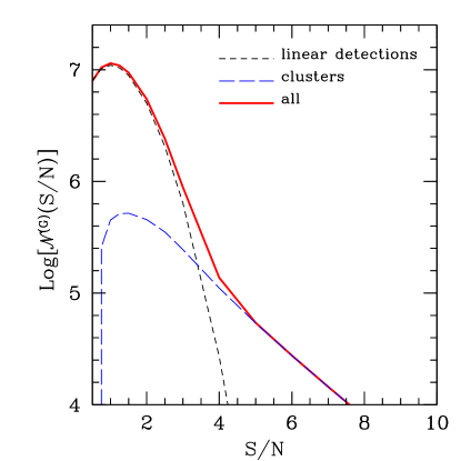
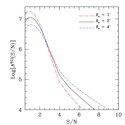
Figure 1: Left panel. The different contributions to the abundance of shear S/N peaks in the reference Gaussian model. The black short dashed line shows the contribution given by LSS projection and data noise, while the blue long dashed line refers to the contribution of the real dark matter clumps. The heavy solid red line is the total count distribution. We adopted optimal filtering with a scale radius of $\theta_{\mathrm{s}}=2^{\prime}$. Right panel. The total number of shear S/N peaks for three different filter scale radii, as labeled.

A method to measure gravitational lensing signatures in optical/near-infrared catalogues of galaxies is the aperture mass (Schneider et al., 1998). It is a weighted average of the tangential component of the shear $\gamma_{\rm t}$ over the position $\boldsymbol{\theta}$ on the sky,

$$A(\boldsymbol{\theta})=\int_{\mathbb{R}^{2}}d^{2}\boldsymbol{\theta}^{\prime}\gamma_{\rm t}(\boldsymbol{\theta}^{\prime},\boldsymbol{\theta})Q(\|\boldsymbol{\theta}^{\prime}-\boldsymbol{\theta}\|)\;,$$ (17)

where the radial filter function $Q$ determines the statistical properties of the estimate $A$ we are interested in. In this paper we aim at constraining the deviations from primordial Gaussianity, which mostly affect the non-linear part of structure formation and thus the high mass end of the mass function. Therefore, we adopted the linear matched filter defined by Maturi et al. (2005) which is designed to maximize the S/N ratio of non linear structures such as galaxy clusters, i.e those structures which are most sensitive to $f_{\mathrm{NL}}$,

$$\hat{Q}(\boldsymbol{\ell})=\alpha\frac{\hat{\tau}(\boldsymbol{\ell})}{P(\ell)},\quad\mbox{with}\quad\alpha^{-1}=\int_{\mathbb{R}^{2}}d^{2}\boldsymbol{\ell}\frac{\left|\hat{\tau}(\boldsymbol{\ell})\right|^{2}}{P(\ell)}\;.$$ (18)

Here the filter is represented in the Fourier space for convenience, $\hat{\tau}(\boldsymbol{\ell})$ is the Fourier transform of the expected shear profile of individual halos, in our case the Fourier transform of the NFW shear profile, and $P(\ell)=P_{\gamma_{\mathrm{t}}}(\ell)+P_{\rm\epsilon}(\ell)$ described in Section 4.2. Note that the shape of the optimal filter depends on the assumed parameters for the NFW density profile, particularly on the angular size corresponding to the scale radius $\theta_{\mathrm{s}}$. Moreover, since the filter is only a radial function, its Fourier transform depends only on $\ell=\|\boldsymbol{\ell}\|$

We further define the variance of the aperture mass estimate $A$ as

$$\sigma_{A}^{2}\equiv\int_{0}^{+\infty}\frac{\ell d\ell}{2\pi}P_{\epsilon}(\ell)|\hat{Q}(\ell)|^{2}\;,$$ (19)

so that it is related only to the non-cosmological signal component, i.e. $P_{\epsilon}$. It is worth mentioning that in practical applications $A$ is approximated as

$$A(\boldsymbol{\theta})=\frac{1}{n}\sum_{i=1}^{n}\epsilon_{{\rm t},i}(\boldsymbol{\theta})Q(\|\boldsymbol{\theta}_{i}-\boldsymbol{\theta}\|)\;,$$ (20)

where $\epsilon_{{\rm t},i}(\boldsymbol{\theta})$ is the tangential ellipticity of a galaxy image located at the position $\boldsymbol{\theta}_{i}$ with respect to $\boldsymbol{\theta}$, and which provides an estimate for $\gamma_{\rm t}$.

4.4 Expected shear peaks number counts

Once the lensing signals and the observational strategy have been defined (see Sections 4.2 and 4.3), the weak lensing number counts can be predicted as the sum of two independent components. On one hand the non-linear structures, i.e. galaxy clusters, whose detection depends on their intrinsic abundance given by the mass function discussed in Section 3.1, and by their observed S/N ratio depending on their expected signal $A$ (see Eq. 17) and variance $\sigma^{2}_{A}$ (see Eq. 19). On the other hand the lensing LSS and instrumental noise which are well approximated by a Gaussian random field and for which their number counts above a specific threshold S/N${}_{\mathrm{th}}=y_{\mathrm{th}}$ can be easily predicted,

$$n_{\mathrm{det}}(y_{\mathrm{th}})=\frac{1}{4\sqrt{2}\pi^{3/2}}\left(\frac{\sigma_{1}}{\sigma_{A}}\right)^{2}\frac{y_{\mathrm{th}}}{\sigma_{A}}\exp\left(-\frac{y_{\mathrm{th}}^{2}}{2\sigma_{A}^{2}}\right)\;,$$ (21)

as shown by Maturi et al. (2010). Here $\sigma_{1}$, defined as

$$\sigma_{1}^{2}=\int_{0}^{+\infty}\frac{\ell^{3}d\ell}{2\pi}P(\ell)|\hat{Q}(\ell)|^{2}\;,$$ (22)

is the LSS plus noise lensing field variance which depends on the observational noise, the convergence power spectrum and the adopted filter.

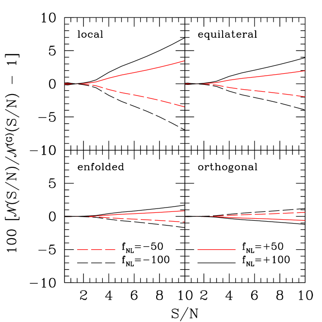
Figure 2: The ratio of the peak number counts in different models with primordial non-Gaussianity to the same quantities in the reference Gaussian $\Lambda$CDM cosmology, as a function of the S/N ratio. Four different non-Gaussian shapes and four different values of $f_{\mathrm{NL}}$ are shown, as labeled in the plot.

Note that, by approximating this therm as a Gaussian random field, the primordial non-Gaussianity is accounted through the LSS power spectrum only so that its leverage is not fully included. For our purpose this is a negligible approximation since we anyway expect this effect to be small and put our final predictions on a conservative side. These two contributions carry complementary cosmological information, thus the statistics of cosmic shear peaks are in principle valuable cosmological tools (Dietrich & Hartlap, 2009).

The two cosmological contributions to the abundance of cosmic shear peaks are exemplified in the left panel of Figure 1 for the reference Gaussian cosmological model. For this Figure and in the rest of the work we adopted the source redshift distribution observationally derived by Benjamin et al. (2007), while their average surface number density is $n_{\mathrm{g}}=40$ arcmin^-2, a level achieved by actual weak lensing surveys and which should be reached by EUCLID (a prediction for a sample of existing and future weak lensing surveys is given by Maturi et al. 2010). As expected, the chance alignment of the LSS dominates the counts at small S/N ratio values, while the contribution coming from the occurrence of real dark matter clumps starts to be relevant at around S/N$\sim 4$ and dominates at higher S/N values. We additionally show in the right panel of the same Figure the total number counts expected for three different scale radii of the optimal filter. As it can be noted, the larger the scale, the larger the contribution of galaxy clusters with respect to the LSS and the noise, although the latter remains always dominant at smaller, but still large, S/N. This behavior is expected because for larger filter scales the detections will have larger areas, thus increasing their blending where their number density is higher, typically at lower S/N. Also, the overall S/N ratio values at higher S/N are expected to be larger, since a larger filter scale implies a better statistic for the background galaxies reducing their shot noise and intrinsic ellipticity. These features are ensured by the adopted optimal filter which maximizes the cluster signal against the one of LSS and noise. In the remainder of this paper we shall refer mainly to a scale radius of $2^{\prime}$, unless explicitly noted otherwise.

5 Signature of primordial non-Gaussianity

The effect of primordial non-Gaussianity on the statistics of shear peaks is exemplified in Figure 2 for the four different non-Gaussian shapes that were discussed in Section 2, and for levels of non-Gaussianity $f_{\mathrm{NL}}=\pm 50$ and $f_{\mathrm{NL}}=\pm 100$. As it can be seen, the effect of non-Gaussianity is more evident at high values of S/N ratio, where it is mostly given by the effect on the mass function of dark matter halos. We remind the reader that our predictions regarding the impact of primordial non-Gaussianity at the S/N ratios dominated by the LSS are conservative as discussed in Section 4.4. Also, as expected, the effect is largest for local non-Gaussianity for which, at high S/N, the counts can be modified by up to $\sim 7\%$ for $f_{\mathrm{NL}}=\pm 100$ and smallest for the orthogonal shape, where it barely reaches $\sim 1\%$. For the orthogonal shape positive values of $f_{\mathrm{NL}}$ provide a decrement in the number counts of shear peaks at high S/N values, while the opposite is true for all other models. This agrees with the behavior of the skewness that has been discussed in Section 2. Although the effect of non-Gaussianity is substantially reduced for shapes different from the local one, it is likely that useful constraints can be put on $f_{\mathrm{NL}}$ for these shapes as well. For instance in the orthogonal case, $f_{\mathrm{NL}}$ is constrained only at the level of a few hundreds by CMB data (Komatsu et al., 2011). Our prediction is compatible with the recent work of Marian et al. (2010), who found an effect on the shear peaks number counts at the level of $\sim 10\%$ for the highest significance detections. Although a direct comparison of the two works is not possible due to different source redshift distributions, different detection schemes, etc., we actually verified that by reducing the scale radius of the optimal filter down to $\theta_{\mathrm{s}}=1^{\prime}$ the effect is raised to $\sim 10\%$. Thus, we conclude that the two works are in broad agreement for the local non-Gaussian model concerning the magnitude of the effect. This is reassuring, since the two results are based on quite different premises and adopt different methodologies: we opted for semi-analytic modeling, while Marian et al. (2010) resorted to the use of cosmological simulations.

In Figure 3 we show the ratio of the peak number counts in non-Gaussian cosmologies with local shape ($f_{\mathrm{NL}}=\pm 10$) to the same quantities in the reference Gaussian case adopting three different values of the power spectrum amplitude $\sigma_{8}$ for all models. We considered $\sim 2\%$ fluctuations in the value of $\sigma_{8}$, comparable with the $1-\sigma$ uncertainty around the fiducial value derived by the WMAP-7 release. Quite unexpectedly, the effect of primordial non-Gaussianity is higher for lower values of $\sigma_{8}$. We interpret this fact as due to the delayed structure formation implied by a lower normalization. This allows the effect of primordial non-Gaussianity on the matter density field to be retained for a longer time by the LSS, with the consequence that the S/N peak number counts are slightly more affected. In other words, since with a lower $\sigma_{8}$ the onset of non-linear evolution is delayed, gravitational clustering has less time to erase the cosmological initial conditions.

6 Cosmological constraints

In this section we use a Fisher-matrix analysis to estimate the confidence level in the $\sigma_{8}-f_{\mathrm{NL}}$ plane, as obtained with the weak lensing number counts.

6.1 Fisher matrix analysis

The Fisher matrix is given by

$$F_{ij}=-\Bigg{\langle}\frac{\partial^{2}\mathcal{L}}{\partial\xi_{i}\partial\xi_{j}}\Bigg{\rangle}\;,$$ (23)

where $\mathcal{L}$ is the logarithm of the likelihood function and $\boldsymbol{\xi}=(\sigma_{8},f_{\mathrm{NL}})$ are the free parameters of the number counts model. In case of a multivariate Gaussian likelihood, the Fisher matrix can be written as

$$F_{ij}=\frac{1}{2}\mathrm{Tr}\left[A_{i}A_{j}+C^{-1}M_{ij}\right]\;,$$ (24)

where $A_{i}=C^{-1}C_{,i}$, $M_{ij}=2(\partial\mu/\partial\xi_{i})(\partial\mu/\partial\xi_{j})$, $C$ is the data covariance matrix, and $\mu$ is the assumed model, i.e. the peaks number counts for different S/N. Here a comma denotes differentiation with respect to the relevant cosmological parameter. Since $C$ has a very weak dependence on the model parameters $\sigma_{8}$ and $f_{\mathrm{NL}}$ the first term in Eq. 24 is negligible because of $C_{,i}$. We evaluated the Fisher matrix at the fiducial point $\sigma_{8}=0.809$ and $f_{\mathrm{NL}}=0$ as measured by WMAP-7 for a standard $\Lambda$CDM model (Komatsu et al., 2011).

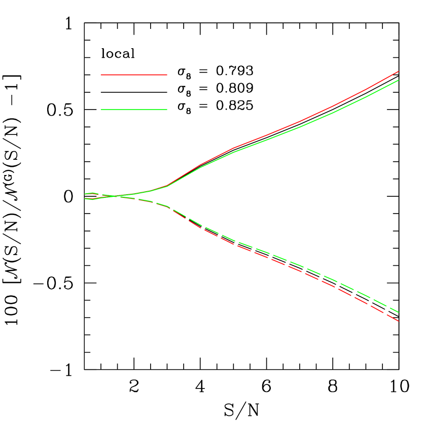
Figure 3: The ratio of the peak number counts in two different non-Gaussian models with local bispectrum shape to the same quantities in the reference Gaussian $\Lambda$CDM cosmology, as a function of the S/N ratio. The upper set of curves refer to $f_{\mathrm{NL}}=10$, while the lower set refers to $f_{\mathrm{NL}}=-10$. Different colors refer to different values of the matter power spectrum normalization $\sigma_{8}$, as labeled.

As discussed in Section 4.4, the number counts model $\mu$ is given by two components. On one hand, the non linear structures whose number counts are independent for different S/N ratio bins and whose covariance contribution is therefore diagonal with a Poissonian amplitude. On the other hand, the contribution given by the LSS and noise for which the number counts are relevant for low S/N ratios up to S/N $\sim 3$, where we expect to have a small but not negligible covariance contribution since different S/N bins can be correlated. To account for the non-diagonal covariance elements, we realized a set of 1000 numerical realizations of weak lensing data, modeled with a Gaussian random field whose power spectrum, $P(\ell)$, is discussed in Section 4.2. As expected the number counts derived from the simulation agrees with the analytical predictions except for very low values of the S/N ratio (S/N $<0.2$) where the analytic approximation fails as discussed by Maturi et al. (2010). In any case these very low S/N are completely negligible for any cosmological analysis.

The total covariance matrix of weak lensing number counts is shown in Figure 4. As expected, it has a strong diagonal component and its off-diagonal terms are small but non negligible only at low S/N ratios. By treating the two components, LSS + noise and galaxy clusters as independent, we do not account for their mutual influence on the final number counts, but this effect is expected to be small because the signature of each cluster affects only few pixels. In any case, this approach is conservative with respect to the final cosmological constraints because we neglect the impact of the detections with high S/N ratios, carriers of the non-Gaussianity signal, on those with lower S/N ratios.

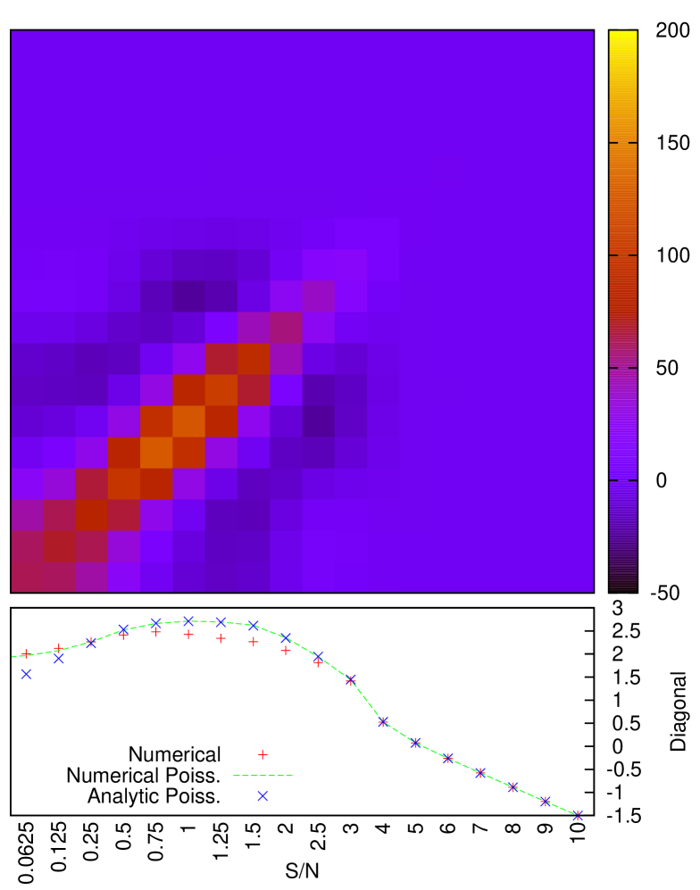
Figure 4: Weak lensing number counts covariance matrix for a $\Lambda$CDM model. The off-diagonal terms are small but not negligible only at low S/N ratios. The bottom panel shows the comparison between the diagonal components of the full covariance matrix derived numerically (shown in the top panel) and what would be expected for ideal number counts with Poisson statistic and statistically independent S/N bins. For high S/N the covariance is diagonal and Poissonian by construction.

6.2 Cosmological constraints on $f_{\mathrm{NL}}$

In this Section we assume the expected performances of the weak lensing survey Euclid (Laureijs, 2009), i.e. a field of view of $20,000$ deg², an average background galaxy number density of $n_{\mathrm{g}}=40$ arcmin^-2 with an intrinsic ellipticity rms of $\sigma_{\mathrm{\epsilon_{s}}}=0.3$, and a redshift distribution similar to the one discussed by Benjamin et al. (2007). The confidence levels are evaluated with the Fisher matrix analysis discussed in Section 6.1. In Figure 5 we compare the confidence regions for the local shape non-Gaussian model obtained first by assuming purely Poissonian independent statistic, i.e. a data covariance having a pure diagonal component with Poissonian amplitude, and then by using the full covariance matrix obtained from the numerical simulations (see Section 6.1). As can be seen, the $1-\sigma$ confidence ellipse is slightly tilted in the latter case with respect to the former, implying a somewhat different direction of degeneracy between the two parameters under consideration. Overall, however, the constraints on the non-Gaussianity level $f_{\mathrm{NL}}$ are basically unchanged, while those on the normalization of the matter power spectrum $\sigma_{8}$ are only very slightly loosened by using the simpler Poisson model. As a consequence, it is safe to state that the final differences between the two approaches are negligible and that for a first fast analysis the simplified approach can be used.

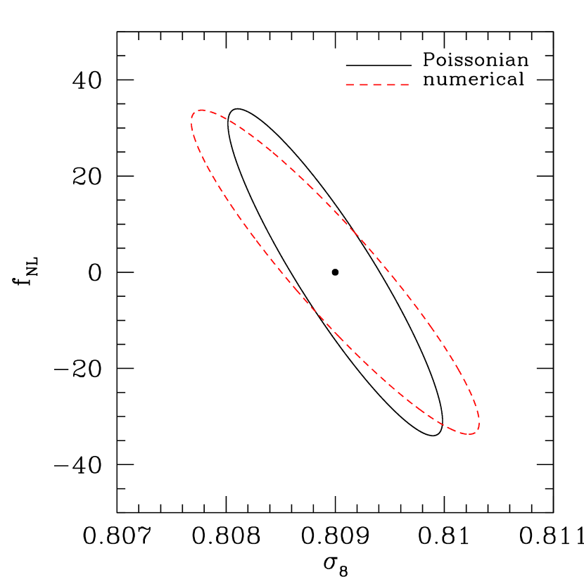
Figure 5: Cosmological $1-\sigma$ confidence levels as obtained for the local shape non-Gaussian model using weak lensing number counts, by assuming both Poissonian statistical independence (Poissonian), and by using the numerical simulations including the full covariance matrix (numerical).

$n_{\mathrm{g}}$	$\Delta\sigma_{8}$	$\Delta f_{\mathrm{NL}}$
20	0.0023	60
40	0.0015	45
80	0.0012	41

$\theta_{\mathrm{s}}$	$\Delta\sigma_{8}$	$\Delta f_{\mathrm{NL}}$
1’	0.0016	57
2’	0.0015	45
4’	0.0015	38

Table 1: Dependence of the $1-\sigma$ joint bounds on the background galaxy number density $n_{\mathrm{g}}$ (left) and on the filter scale radius, $\theta_{\mathrm{s}}$ (right). The fiducial model with $\sigma_{8}=0.809$ and $f_{\mathrm{NL}}=0$ is adopted.

Given that, we used the first approach to estimate the Cramér-Rao bounds on $\sigma_{8}$ and $f_{\mathrm{NL}}$ at $1-\sigma$ level for different survey depths, i.e. different galaxies number densities, and for different filter scales as shown in Table 1. In order to save computational time, the full data covariance has been used only for the final results reported below. The results are evaluated for a survey sky coverage of $20,000$ deg² and scale with the square root of the survey area. The constraints on both $f_{\mathrm{NL}}$ and $\sigma_{8}$ improve with increasing number density of background sources. However only a marginal benefit is obtained by increasing the number density over $40$ arcmin^-2. In other words, in terms of joint constraints for the level of non-Gaussianity and amplitude of the matter power spectrum, it does not pay off to increase the depth of the survey beyond what is already planned for Euclid. Concerning the scale radius of the optimal filter, by increasing it we get a significant tightening of the constraints on $f_{\mathrm{NL}}$, while those on $\sigma_{8}$ are almost insensitive to it.

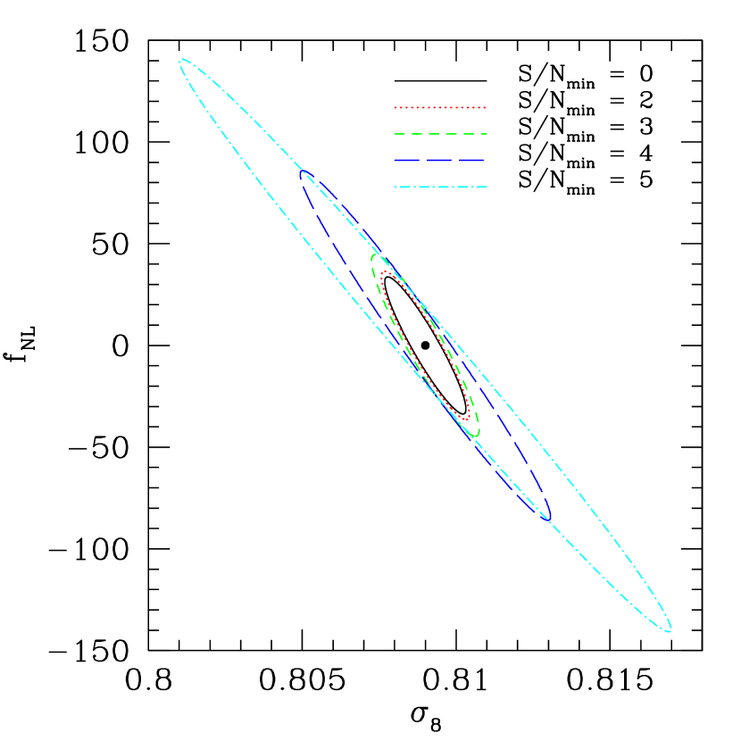
Figure 6: Confidence contours for the local shape non-Gaussian model, with different lower S/N cut-off limits. This shows the information lost by cutting the data at different S/N ratios.

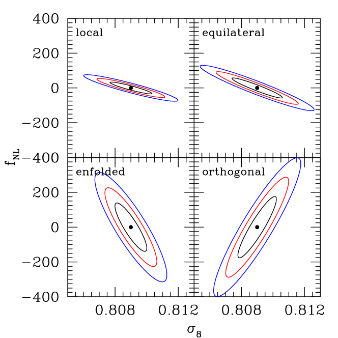
Figure 7: Confidence regions for the four adopted models with non-Gaussian initial conditions. We report results for the local (top left), equilateral (top right), enfolded (bottom left) anqd orthogonal (bottom right) primordial bispectrum shapes. The three contours in each panel refer to $68.3\%$, $95.4\%$, and $99.7\%$ confidence levels.

Now that we have an overall picture of the dependence on the survey characteristics, we used the numerical simulations including the full covariance matrix to obtain our final results. In Figure 6 we show the $1-\sigma$ confidence levels in the $\sigma_{8}-f_{\mathrm{NL}}$ plane obtained for the non-Gaussian model with local shape when different minimum S/N ratios are considered. It is in fact common practice for actual applications to use only those detections with S/N larger then S/N${}_{\mathrm{min}}=3-5$ in the attempt to isolate galaxy clusters from all other signal components. Here we show how the cut-off level affects the final results. The related loss of information happens because the presence of non linear structures affects the statistic of weak lensing maps also at lower signal to noise ratios where they cannot be seen as clear single detections but where their presence is still visible. Moreover, although this effect is negligible for the $f_{\mathrm{NL}}$ estimates, chance projection of the LSS dominates at these small S/N values, and still contains cosmological information. Figure 6 shows that adopting a conservative choice for the minimum S/N value can results in a loss of constraining power of a factor $\sim 3$ on $f_{\mathrm{NL}}$ and a factor of $\sim 4$ on $\sigma_{8}$. Thus, particular care have to be used when defining the detection selection criteria since data can be fully exploited only if lower S/N levels, e.g. S/N${}_{\mathrm{min}}\sim 2$, are used. This would be possible only if a deep statistical understanding of data is achieved together with a detailed modeling. A tentative to go in this direction is provided by the analytic prediction for weak lensing number counts proposed by Maturi et al. (2010) but which still needs to improve some of the adopted approximations.

Finally we show in Figures 7 the constraints for $68.3\%$, $95.4\%$ and $99.7\%$ confidence levels with S/N${}_{\mathrm{min}}=0$ for the four different primordial bispectrum shapes discussed in Section 2. We adopted the optimal filter with scale of $\theta_{\mathrm{s}}=2^{\prime}$. As one could naively expect, while the constraints on $\sigma_{8}$ are rather insensitive to the adopted shape of the primordial bispectrum, the constraints on $f_{\mathrm{NL}}$ vary widely with it. Particularly, while the $1-\sigma$ error $\Delta f_{\mathrm{NL}}$ is at the level of a few tens for the local and equilateral shapes, it grows up to $\sim 100-200$ for the enfolded and orthogonal shapes. These constraints are not competitive with what is expected by future CMB and galaxy clustering probes, and are only comparable with the expected performance of the weak lensing power spectrum (Fedeli & Moscardini, 2010) analysis. The main reason for this results is that in this work we did not use the full redshift information which is otherwise included in the other works and which could be included by the use of lensing tomography. Recently, Fedeli et al. (2010) have shown that using the correlation function of weak lensing-selected clusters it is possible to push the bounds on $f_{\mathrm{NL}}$ below what would be achieved without redshift information. In addition, it is likely that a combination of these diverse probes can reduce the error on $f_{\mathrm{NL}}$ substantially. We plan to investigate this synergy in a future work.

The constraints on the amplitude of the matter power spectrum, $\Delta\sigma_{8}\sim 10^{-3}$ are themselves quite competitive. For instance, recently Wang et al. (2010) forecasted an error on $\sigma_{8}$ of $\sim 7\times 10^{-2}$ by using the shape and position of the Baryon Acoustic Oscillation measured by Euclid. Despite the fact that Wang et al. (2010) let all the cosmological parameters free to vary, while we limit our analysis to $f_{\mathrm{NL}}$ and $\sigma_{8}$, these numbers argue for our constraints on the amplitude of the matter power spectrum being sound.

The degeneracy between the level of primordial non-Gaussianity and the amplitude of the matter power spectrum is also easy to understand, since increases in both $f_{\mathrm{NL}}$ and $\sigma_{8}$ bring an increment in the large scale matter power spectrum and the occurrence of massive dark matter halos. The only exception to this is given by the orthogonal model, because in this case a positive $f_{\mathrm{NL}}$ implies a decrement in both the abundance of cosmic structures and the large scale bias of dark matter halos. For further clarity, in Figure 8 we show the $1-\sigma$ confidence levels in the $\sigma_{8}-f_{\mathrm{NL}}$ plane for the four primordial bispectrum shapes considered in this work together. This Figure allows a more direct comparison between the different models, and highlights the differences in constraining the level of primordial non-Gaussianity between them.

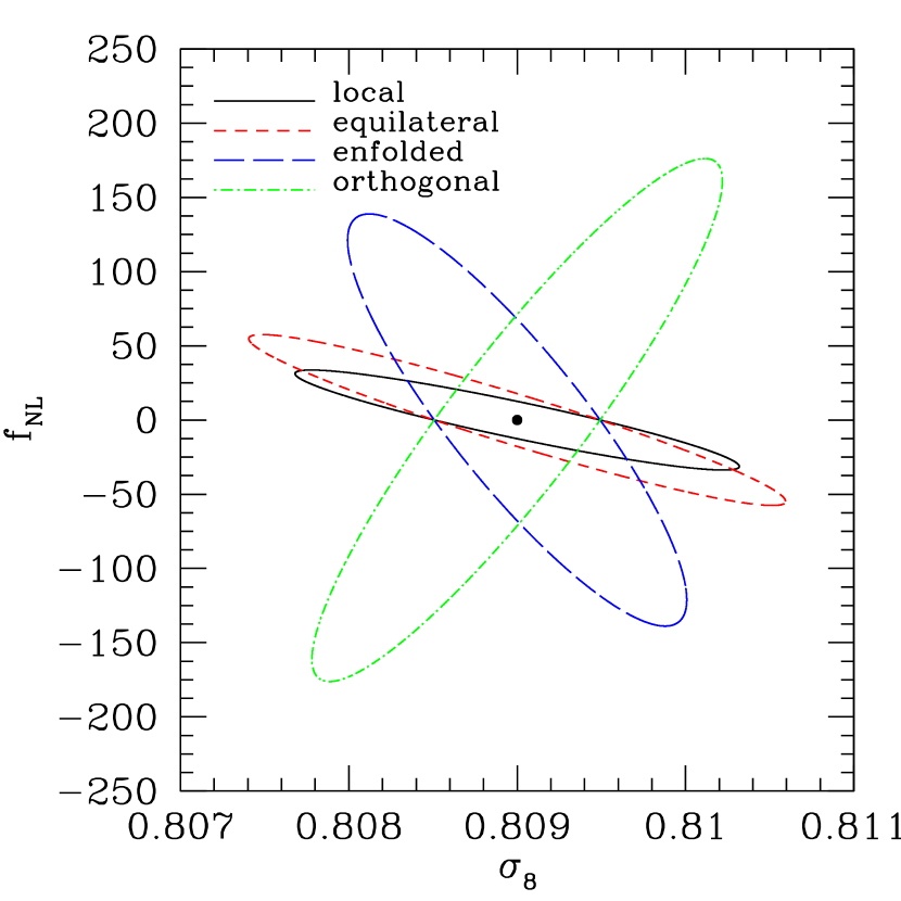
Figure 8: The $1-\sigma$ confidence levels in the $\sigma_{8}-f_{\mathrm{NL}}$ plane for all the four shapes of the primordial bispectrum considered in this work, as labeled

7 Summary and conclusions

The abundance of S/N peaks in cosmic shear maps contains cosmological information through the mass function of large dark matter clumps and the projection of the large scale matter distribution. We considered the effect of deviations from primordial Gaussianity on this particular weak lensing statistic. Analytic modeling of the galaxy cluster mass function, the large scale halo bias, and the fully non-linear power spectrum of dark matter was implemented, where the effect of primordial non-Gaussianity could be straightforwardly introduced. We predicted analytically and through simple numerical simulations the expected weak lensing peaks number counts and covariance for different weak lensing filters. We then performed a Fisher matrix analysis in order to forecast the constraints on the level of primordial non-Gaussianity $f_{\mathrm{NL}}$ and the amplitude of the matter power spectrum $\sigma_{8}$ that could be expected by counting the cosmic shear peaks for different survey configurations, i.e. depth and field of view, in particular for the half-sky maps expected by the proposed ESA space mission Euclid. Our principal results can be summarized as follows.

• Primordial non-Gaussianity affects mainly the high S/N part of the shear peak number counts, where the signal is dominated by the occurrence of real cluster-sized dark matter halos. For the local primordial bispectrum shape and according to the adopted weak lensing filter the number counts can be modified by $\sim 3-4\%$ at S/N $\gtrsim 10$ if $|f_{\mathrm{NL}}|=50$, and by up to $\sim 10\%$ for $|f_{\mathrm{NL}}|=100$. For the enfolded and orthogonal bispectrum shapes, the modification reaches at most $\sim 1-2\%$ for $|f_{\mathrm{NL}}|=100$.

• Generically an increment in $f_{\mathrm{NL}}$ corresponds to an increment in the number counts of cosmic shear peaks, and the other way round, compatibly with the effect of primordial non-Gaussianity on the cluster mass function. The exception to this is given by the orthogonal model, for which it is known that the skewness and scale-dependent bias correction are negative for positive $f_{\mathrm{NL}}$, and vice-versa.

• We show that considering only cosmic shear peaks with S/N larger than $3-5$, as it is costume in actual applications, leads to a loss of cosmological information because the LSS and, more importantly, the low mass clusters contributions are ignored. In particular the latter is important in constraining $f_{\mathrm{NL}}$ even if these structures cannot be detected individually. Thus, data can be better exploited if lower S/N levels, e.g. S/N${}_{\mathrm{min}}\lesssim 2$, are used. For this achievement, a deep statistical understanding and a detailed data modeling are necessary.

• In terms of joint constraints for $f_{\mathrm{NL}}$ and $\sigma_{8}$ only a marginal benefit is obtained by increasing the background galaxy number density above $40$ arcmin^-2, while it is more convenient to go for wider fields of view. By increasing the scale radius of the optimal filter we obtained a significant improvement for the $f_{\mathrm{NL}}$ constraints, while those on $\sigma_{8}$ are almost unaffected.

• Counting cosmic shear peaks in future wide field optical/near-infrared surveys on the model of Euclid can constrain $f_{\mathrm{NL}}$ to the level of a few tens for the local and orthogonal shapes, and to the level of $\sim 100-200$ for the enfolded and orthogonal shapes. Constraints on $\sigma_{8}$ are at the level of $\sim 10^{-3}$ and are instead rather insensitive to the assumed shape of the primordial bispectrum.

The results presented in this work show that the abundance of cosmic shear peaks can be a powerful mean for constraining cosmology. Forecasted errors on the level of primordial non-Gaussianity for a Euclid-like survey are competitive with similar constraints given by weak lensing tomography and the correlation function of weak lensing selected galaxy clusters. At the same time, counting cosmic shear peaks irrespective of their nature is much easier and less subject to systematics compared with other probes where the nature of each lensing peak, resulting by LSS or galaxy clusters, has to be determined. Our findings outline once more the great advance in understanding the physics of the primordial Universe that is expected thanks to future wide field imaging surveys.

References

- Afshordi & Tolley (2008) Afshordi, N. & Tolley, A. J. 2008, \prd, 78, 123507
- Alishahiha et al. (2004) Alishahiha, M., Silverstein, E., & Tong, D. 2004, \prd, 70, 123505
- Amara & Refregier (2004) Amara, A. & Refregier, A. 2004, \mnras, 351, 375
- Arkani-Hamed et al. (2004) Arkani-Hamed, N., Creminelli, P., Mukohyama, S., & Zaldarriaga, M. 2004, Journal of Cosmology and Astro-Particle Physics, 4, 1
- Assadullahi et al. (2007) Assadullahi, H., Väliviita, J., & Wands, D. 2007, \prd, 76, 103003
- Avila-Reese et al. (2003) Avila-Reese, V., Colín, P., Piccinelli, G., & Firmani, C. 2003, \apj, 598, 36
- Babich et al. (2004) Babich, D., Creminelli, P., & Zaldarriaga, M. 2004, Journal of Cosmology and Astro-Particle Physics, 8, 9
- Bardeen et al. (1986) Bardeen, J. M., Bond, J. R., Kaiser, N., & Szalay, A. S. 1986, \apj, 304, 15
- Bartelmann (1996) Bartelmann, M. 1996, \aap, 313, 697
- Bartelmann & Schneider (2001) Bartelmann, M. & Schneider, P. 2001, \physrep, 340, 291
- Bartolo et al. (2004) Bartolo, N., Komatsu, E., Matarrese, S., & Riotto, A. 2004, \physrep, 402, 103
- Bartolo et al. (2002) Bartolo, N., Matarrese, S., & Riotto, A. 2002, \prd, 65, 103505
- Benjamin et al. (2007) Benjamin, J., Heymans, C., Semboloni, E., et al. 2007, \mnras, 381, 702
- Bernardeau & Uzan (2002) Bernardeau, F. & Uzan, J. 2002, \prd, 66, 103506
- Blinnikov & Moessner (1998) Blinnikov, S. & Moessner, R. 1998, \aaps, 130, 193
- Carbone et al. (2010) Carbone, C., Mena, O., & Verde, L. 2010, \jcap, 7, 20
- Carbone et al. (2008) Carbone, C., Verde, L., & Matarrese, S. 2008, \apjl, 684, L1
- Chen (2005) Chen, X. 2005, \prd, 72, 123518
- Chen (2010) Chen, X. 2010, ArXiv e-prints, 1002.1416
- Chen et al. (2007) Chen, X., Huang, M., Kachru, S., & Shiu, G. 2007, Journal of Cosmology and Astro-Particle Physics, 1, 2
- Cooray (2006) Cooray, A. 2006, Physical Review Letters, 97, 261301
- Cooray & Sheth (2002) Cooray, A. & Sheth, R. 2002, \physrep, 372, 1
- Creminelli et al. (2010) Creminelli, P., D’Amico, G., Musso, M., Noreña, J., & Trincherini, E. 2010, ArXiv e-prints, 1011.3004
- Creminelli et al. (2007) Creminelli, P., Senatore, L., Zaldarriaga, M., & Tegmark, M. 2007, Journal of Cosmology and Astro-Particle Physics, 3, 5
- Crociani et al. (2009) Crociani, D., Moscardini, L., Viel, M., & Matarrese, S. 2009, \mnras, 394, 133
- Dalal et al. (2008) Dalal, N., Doré, O., Huterer, D., & Shirokov, A. 2008, \prd, 77, 123514
- Desjacques & Seljak (2010) Desjacques, V. & Seljak, U. 2010, Classical and Quantum Gravity, 27, 124011
- Dietrich & Hartlap (2009) Dietrich, J. P. & Hartlap, J. 2009, \mnras, 1893
- Eisenstein & Hu (1998) Eisenstein, D. J. & Hu, W. 1998, \apj, 496, 605
- Falk et al. (1993) Falk, T., Rangarajan, R., & Srednicki, M. 1993, \apjl, 403, L1
- Fedeli et al. (2010) Fedeli, C., Carbone, C., Moscardini, L., & Cimatti, A. 2010, ArXiv e-prints 1012.2305
- Fedeli & Moscardini (2010) Fedeli, C. & Moscardini, L. 2010, \mnras, 405, 681
- Fedeli et al. (2009) Fedeli, C., Moscardini, L., & Matarrese, S. 2009, \mnras, 397, 1125
- Fergusson et al. (2010) Fergusson, J. R., Liguori, M., & Shellard, E. P. S. 2010, \prd, 82, 023502
- Fergusson & Shellard (2009) Fergusson, J. R. & Shellard, E. P. S. 2009, \prd, 80, 043510
- Gangui et al. (1994) Gangui, A., Lucchin, F., Matarrese, S., & Mollerach, S. 1994, \apj, 430, 447
- Grossi et al. (2008) Grossi, M., Branchini, E., Dolag, K., Matarrese, S., & Moscardini, L. 2008, \mnras, 390, 438
- Grossi et al. (2007) Grossi, M., Dolag, K., Branchini, E., Matarrese, S., & Moscardini, L. 2007, \mnras, 382, 1261
- Grossi et al. (2009) Grossi, M., Verde, L., Carbone, C., et al. 2009, \mnras, 398, 321
- Guth (1981) Guth, A. H. 1981, \prd, 23, 347
- Hikage et al. (2008) Hikage, C., Coles, P., Grossi, M., et al. 2008, \mnras, 385, 1613
- Holman & Tolley (2008) Holman, R. & Tolley, A. J. 2008, Journal of Cosmology and Astro-Particle Physics, 5, 1
- Jenkins et al. (2001) Jenkins, A., Frenk, C. S., White, S. D. M., et al. 2001, \mnras, 321, 372
- Jeong & Komatsu (2009) Jeong, D. & Komatsu, E. 2009, \apj, 703, 1230
- Komatsu et al. (2009) Komatsu, E., Dunkley, J., Nolta, M. R., et al. 2009, \apjs, 180, 330
- Komatsu et al. (2011) Komatsu, E., Smith, K. M., Dunkley, J., et al. 2011, \apjs, 192, 18
- Komatsu & Spergel (2001) Komatsu, E. & Spergel, D. N. 2001, \prd, 63, 063002
- Laureijs (2009) Laureijs, R. 2009, ArXiv e-prints, 0912.0914
- Li et al. (2008) Li, M., Wang, T., & Wang, Y. 2008, Journal of Cosmology and Astro-Particle Physics, 3, 28
- Linde (1982) Linde, A. D. 1982, Physics Letters B, 108, 389
- LoVerde et al. (2008) LoVerde, M., Miller, A., Shandera, S., & Verde, L. 2008, Journal of Cosmology and Astro-Particle Physics, 4, 14
- Ma & Fry (2000) Ma, C.-P. & Fry, J. N. 2000, \apj, 543, 503
- Maggiore & Riotto (2010a) Maggiore, M. & Riotto, A. 2010a, \apj, 711, 907
- Maggiore & Riotto (2010b) Maggiore, M. & Riotto, A. 2010b, \apj, 717, 515
- Maggiore & Riotto (2010c) Maggiore, M. & Riotto, A. 2010c, \apj, 717, 526
- Marian et al. (2010) Marian, L., Hilbert, S., Smith, R. E., Schneider, P., & Desjacques, V. 2010, ArXiv e-prints, 1010.5242
- Matarrese & Verde (2008) Matarrese, S. & Verde, L. 2008, \apjl, 677, L77
- Matarrese et al. (2000) Matarrese, S., Verde, L., & Jimenez, R. 2000, \apj, 541, 10
- Mathis et al. (2004) Mathis, H., Diego, J. M., & Silk, J. 2004, \mnras, 353, 681
- Matsubara (2003) Matsubara, T. 2003, \apj, 584, 1
- Maturi et al. (2010) Maturi, M., Angrick, C., Pace, F., & Bartelmann, M. 2010, \aap, 519, A23+
- Maturi et al. (2005) Maturi, M., Meneghetti, M., Bartelmann, M., Dolag, K., & Moscardini, L. 2005, \aap, 442, 851
- McDonald (2008) McDonald, P. 2008, \prd, 78, 123519
- Meerburg et al. (2009) Meerburg, P. D., van der Schaar, J. P., & Corasaniti, S. P. 2009, Journal of Cosmology and Astro-Particle Physics, 5, 18
- Meneghetti et al. (2003) Meneghetti, M., Bartelmann, M., & Moscardini, L. 2003, \mnras, 340, 105
- Messina et al. (1990) Messina, A., Moscardini, L., Lucchin, F., & Matarrese, S. 1990, \mnras, 245, 244
- Moscardini et al. (1991) Moscardini, L., Matarrese, S., Lucchin, F., & Messina, A. 1991, \mnras, 248, 424
- Navarro et al. (1996) Navarro, J. F., Frenk, C. S., & White, S. D. M. 1996, \apj, 462, 563
- Navarro et al. (1997) Navarro, J. F., Frenk, C. S., & White, S. D. M. 1997, \apj, 490, 493
- Pillepich et al. (2009) Pillepich, A., Porciani, C., & Hahn, O. 2009, \mnras, 1959
- Pillepich et al. (2007) Pillepich, A., Porciani, C., & Matarrese, S. 2007, \apj, 662, 1
- Press & Schechter (1974) Press, W. H. & Schechter, P. 1974, \apj, 187, 425
- Salopek & Bond (1990) Salopek, D. S. & Bond, J. R. 1990, \prd, 42, 3936
- Sasaki et al. (2006) Sasaki, M., Väliviita, J., & Wands, D. 2006, \prd, 74, 103003
- Schneider et al. (1998) Schneider, P., van Waerbeke, L., Jain, B., & Kruse, G. 1998, \mnras, 296, 873
- Seery & Lidsey (2005) Seery, D. & Lidsey, J. E. 2005, Journal of Cosmology and Astro-Particle Physics, 6, 3
- Sefusatti & Komatsu (2007) Sefusatti, E. & Komatsu, E. 2007, \prd, 76, 083004
- Seljak (2000) Seljak, U. 2000, \mnras, 318, 203
- Senatore et al. (2010) Senatore, L., Smith, K. M., & Zaldarriaga, M. 2010, Journal of Cosmology and Astro-Particle Physics, 1, 28
- Sheth et al. (2001) Sheth, R. K., Mo, H. J., & Tormen, G. 2001, \mnras, 323, 1
- Sheth & Tormen (2002) Sheth, R. K. & Tormen, G. 2002, \mnras, 329, 61
- Silverstein & Tong (2004) Silverstein, E. & Tong, D. 2004, \prd, 70, 103505
- Slosar et al. (2008) Slosar, A., Hirata, C., Seljak, U., Ho, S., & Padmanabhan, N. 2008, Journal of Cosmology and Astro-Particle Physics, 8, 31
- Smith et al. (2010) Smith, R. E., Desjacques, V., & Marian, L. 2010, ArXiv e-prints, 1009.5085
- Starobinskiǐ (1979) Starobinskiǐ, A. A. 1979, Soviet Journal of Experimental and Theoretical Physics Letters, 30, 682
- Sugiyama (1995) Sugiyama, N. 1995, \apjs, 100, 281
- Tinker et al. (2008) Tinker, J., Kravtsov, A. V., Klypin, A., et al. 2008, \apj, 688, 709
- Verde & Matarrese (2009) Verde, L. & Matarrese, S. 2009, \apjl, 706, L91
- Verde et al. (2000) Verde, L., Wang, L., Heavens, A. F., & Kamionkowski, M. 2000, \mnras, 313, 141
- Viel et al. (2009) Viel, M., Branchini, E., Dolag, K., et al. 2009, \mnras, 393, 774
- Wagner et al. (2010) Wagner, C., Verde, L., & Boubekeur, L. 2010, \jcap, 10, 22, 1006.5793
- Wang et al. (2010) Wang, Y., Percival, W., Cimatti, A., et al. 2010, \mnras, 409, 737
- Warren et al. (2006) Warren, M. S., Abazajian, K., Holz, D. E., & Teodoro, L. 2006, \apj, 646, 881
- Weinberg & Cole (1992) Weinberg, D. H. & Cole, S. 1992, \mnras, 259, 652