Enabling parallel computing in CRASH

Abstract

We present the new parallel version (pCRASH2) of the cosmological radiative transfer code CRASH2 for distributed memory supercomputing facilities. The code is based on a static domain decomposition strategy inspired by geometric dilution of photons in the optical thin case that ensures a favourable performance speed-up with increasing number of computational cores. Linear speed-up is ensured as long as the number of radiation sources is equal to the number of computational cores or larger. The propagation of rays is segmented and rays are only propagated through one sub-domain per time step to guarantee an optimal balance between communication and computation. We have extensively checked pCRASH2 with a standardised set of test cases to validate the parallelisation scheme. The parallel version of CRASH2 can easily handle the propagation of radiation from a large number of sources and is ready for the extension of the ionisation network to species other than hydrogen and helium.

1 Introduction

The field of computational cosmology has developed dramatically during the last decades. Especially the evolution of the baryonic physics has played an important role in the understanding of the transition from the smooth early universe to the structured present one. We are especially interested in the development of the intergalactic ionising radiation field and the thermodynamic state of the baryonic gas. First measurements of the epoch of reionisation are soon expected from new radio interferometers such as LOFAR or MWA, which will become operative within one year. The interpretation of these measurements requires, among others, a treatment of radiative transfer coupled to cosmological structure formation.

Over the last decade, many different numerical algorithms have emerged, allowing the continuum radiative transfer equation to be solved for arbitrary geometries and density distributions. A substantial fraction of the codes solve the radiative transfer (RT) equation on regular or adaptive grids (for example see Gnedin & Abel (2001); Abel & Wandelt (2002); Razoumov et al. (2002); Mellema et al. (2006)). Other codes developed schemes that introduce RT into the SPH formalism (Pawlik & Schaye, 2008; Petkova & Springel, 2009; Hasegawa & Umemura, 2010) or into unstructured grids (Ritzerveld et al., 2003; Paardekooper et al., 2010) The large amount of different numerical strategies prompted a comparison of the different methods on a standardised problem set. For results of this comparison project we refer the reader to Iliev et al. (2006) and Iliev et al. (2009), where the performance of 11 cosmological RT and 10 radiation hydrodynamic codes are systematically studied.

Our straightforward and very flexible approach is based on a ray-tracing Monte Carlo (MC) scheme. Exploiting the particle nature of a radiation field, it is possible to solve the RT equation for arbitrary three-dimensional Cartesian grids and an arbitrary distribution of absorbers. By describing the radiation field in terms of photons, which are then grouped into photon packets containing a large number of photons each, it is possible to solve the RT along one dimensional rays. With this strategy the explicit dependence on direction and position can be avoided. Instead of directly solving for the intensity field only the interaction of photons with the gas contained in the cells needs to be modelled, as done in long and short characteristics algorithms (Mellema et al., 2006; Rijkhorst et al., 2006; Whalen & Norman, 2006). MC ray-tracing schemes differ from short and long characteristic methods. Instead of casting rays through the grid to each cell in the computational domain, the radiation field is described statistically by shooting rays in random directions from the source. However unlike in fully Monte Carlo transport schemes where the location of the photon matter interaction is determined by sampling the packet’s mean free path, the packets are propagated and attenuated through the grid from cell to cell along rays until all the photons are absorbed or the packets exits the computational domain. This allows for an efficient handling of multiple point sources and diffuse radiation fields, such as recombination radiation or the ultraviolet (UV) background field. Additionally this statistical approach easily allows for sources with anisotropic radiation. A drawback of any Monte Carlo sampling method however is the introduction of numerical noise. By increasing the number of rays used for the sampling of the radiation field though, numerical noise can be reduced at cost of computational resources.

Such a ray-tracing MC scheme has been successfully implemented in our code CRASH2, which is, to date, one of the main references among RT numerical methods used in cosmology. CRASH was first introduced by Ciardi et al. (2001) to follow the evolution of hydrogen ionisation for multiple sources under the assumption that hydrogen has a fixed temperature. Then the code has been further developed by including the physics of helium chemistry, temperature evolution, and background radiation (Maselli et al., 2003; Maselli & Ferrara, 2005). In its latest version, CRASH2, the numerical noise by the MC sampling has been greatly reduced through the introduction of coloured photon packets (Maselli et al., 2009).

The problems that are being solved with cosmological RT codes become larger and larger, in terms of computational cost. Especially, the study of reionisation is a demanding task, since a vast number of sources and large volumes are needed to properly model the era of reionisation (Baek et al., 2009; McQuinn et al., 2007; Trac & Cen, 2007; Iliev et al., 2006). Furthermore the addition of more and more physical processes to CRASH2 requires increased precision in the solution. To study such computationally demanding models with CRASH2, the code needs support for parallel distributed memory computers. In this paper we present the parallelisation strategy adopted for our MPI parallel version of the latest version of the serial CRASH2 code, which we call pCRASH2.

The paper is structured as follows. First we give a brief summary of the serial CRASH2 implementation in Section 2. In Section 3 we review the existing parallelisation strategies for MC ray-tracing codes and describe the approach taken by pCRASH2. In Section 4 we extensively test the parallel implementation against standardised test cases. We further study the scaling properties of the parallel code in Section 4.3 and summarise our results in Section 5. Throughout this paper we assume $h=0.7$.

2 CRASH2: Summary of the Algorithm

In this Section we briefly summarise the CRASH2 code. A complete description of the algorithm is found in Maselli et al. (2003) and in Maselli et al. (2009), with an additional detailed description of the implementation for the background radiation field given in Maselli & Ferrara (2005). We refer the interested reader to these papers for a full description of CRASH2.

CRASH2 is a Monte-Carlo long-characteristics continuum RT code, which is based on ray-tracing techniques on a three-dimensional Cartesian grid. Since many of the processes involved in RT, like recombination emission or scattering processes, are probabilistic, Monte Carlo methods are a straight forward choice in capturing these processes adequately. CRASH2 therefore relies heavily on the sampling of various probability distribution functions (PDFs) which describe several physical processes such as the distribution of photons from a source, reemission due to electron recombination, and the emission of background field photons. The numerical scheme follows the propagation of ionising radiation through an arbitrary H/He static density field and captures the evolution of the thermal and ionisation state of the gas on the fly. The typical RT effects giving rise to spectral filtering, shadowing and self-shielding are naturally captured by the algorithm.

The radiation field is discretised into distinct energy packets, which can be seen as packets of photons. These photon packets are characterised by a propagation direction and their spectral energy content $E(\nu_{j})$ as a function of discrete frequency bins $\nu_{j}$. Both the radiation fields arising from multiple point sources, located arbitrarily in the box, and from diffuse radiation fields such as the background field or radiation produced by recombining electrons are discretised into such photon packets.

Each source emits photon packets according to its luminosity $L_{s}$ at regularly spaced time intervals $\Delta t$. The total energy radiated by one source during the total simulation time $t_{\mathrm{sim}}$ is $E_{s}=\int_{0}^{t_{\mathrm{sim}}}L_{s}(t_{s}){\mathrm{d}}t_{s}$. For each source, $E_{s}$ is distributed in $N_{p}$ photon packets. The energy emitted per source in one time step is further distributed according to the source’s spectral energy distribution function into $N_{\nu}$ frequency bins $\nu_{j}$. We call such a photon packet a coloured packet. Then for each coloured packet produced by a source in one time step, an emission direction is determined according to the angular emission PDF of the source. Thus $N_{p}$ is the main control parameter in CRASH2 governing both the time resolution as well as the spatial resolution of the radiation field.

After a source produced a coloured packet, it is propagated through the given density field. Every time a coloured packet traverses a cell $k$, the length of the path within each crossed cell is calculated and the cell’s optical depth to ionising continuum radiation $\tau_{c}^{k}$ is determined by summing up the contribution of the different absorber species (H i, He i, He ii). The total number of photons absorbed in cell $k$ per frequency bin $\nu_{j}$ is thus

$$N_{A,\gamma}^{(k)}=N_{T,\gamma}^{(k-1)}\left(\nu_{j}\right)\left[1-\mathrm{e}^{-\tau_{c}^{k}\left(\nu_{j}\right)}\right]$$ (1)

where $N_{T,\gamma}^{(k-1)}$ is the number of photons transmitted through cell $k-1$. The total number of absorbed photons is then distributed to the various species according to their contribution to the cell’s total optical depth. Before the packet is propagated to the next cell, the cell’s ionisation fractions and temperature are updated by solving the ionisation network for $\Delta x_{\mathrm{{\mathbf{H\,\text{{i}}}}}}$, $\Delta x_{\mathrm{{\mathbf{He\,\text{{i}}}}}}$, $\Delta x_{\mathrm{{\mathbf{He\,\text{{ii}}}}}}$, and by solving for changes in the cells temperature $\Delta T$ due to photo-heating and the changes in the number of free particles of the plasma. The number of recombining electrons $N_{\mathrm{rec}}$ is recorded as well and is used for the production of the diffuse recombination radiation. In addition to the discrete process of photoionisation, CRASH2 includes various continuous ionisation and cooling processes in the ionisation network (bremsstrahlung, Compton cooling/heating, collisional ionisation, collisional ionisation cooling, collisional excitation cooling, and recombination cooling).

After these steps, the photon packet is propagated to the next cell and these steps are repeated until the packet is either extinguished or, if periodic boundary conditions are not considered, until it leaves the simulation box. At fixed time intervals $\Delta t_{\mathrm{rec}}$, the grid is checked for any cell that has experienced enough recombination events to reach a certain threshold criteria $N_{\mathrm{rec}}\geq f_{\mathrm{rec}}N_{a}$, where $N_{a}$ is the total number of species ”$a$” atoms and $f_{\mathrm{rec}}\in[0,1]$ is the recombination threshold. If the reemission criteria is fulfilled, a recombination emission packet is produced by sampling the probability that a photon with energy larger than the ionisation threshold of H or He is emitted. The spectral energy distribution of the photon packet is determined by the Milne spectrum (Mihalas & Weibel Mihalas, 1984). After the reemission event, the cell’s counter for recombination events is put to zero and the photon packet is propagated through the box.

For further details on the algorithm and its implementation, we again refer the reader to the papers mentioned above.

3 Parallelisation Strategy

Monte Carlo radiation transfer methods are a powerful and easy to implement class of algorithms that enable a determination of the radiation intensity in a simulation grid or on detectors (such as CCDs or photographic plates). Photons originating at sources are followed through the computational domain, i.e. the whole simulation box, up to a grid cell or the detector in a stochastic fashion (Jonsson, 2006; Juvela, 2005; Bianchi et al., 1996). If only the intensity field is of interest, a straight forward parallelisation strategy is to mirror the computational domain and all its sources on multiple processors, so that every processor holds a copy of the same data set. Then each node (a node can consist of multiple computational cores) propagates its own subset of the global photon sample through the domain until the grid boundary or the detector plane is reached. At the end, the photon counts which were determined independently on each node or core are gathered to the master node and are summed up to obtain the final intensity map (Marakis et al., 2001). This technique is also known as reduction. This strategy however only works if the memory requirement of the problem setup fits the memory available to each core. What if the computational core’s memory does not allow for duplication of the data?

To solve this problem, hybrid solutions have been proposed, where the computational domain is decomposed into sub-domains and distributed to multiple task farms (Alme et al., 2001). Each task farm is a collection of nodes and/or cores working on the same sub-domain. A task farm can either reside on just one computational node, or it can span over multiple nodes. Each entity in the task farm propagates photons individually through the sub-domain until they reach the border or a detector. If photons reach the border of the sub-domain, they are communicated to the task farm containing the neighbouring sub-domain. The cumulated intensity map is obtained by first aggregating the different contributions of the computational cores in each task farm, and then by merging the solutions of the individual task farms. The hybrid use of distributed (multiple nodes per task farm) and shared memory concepts (domain is shared between all cores per task farm) allows to balance the amount of communication that is needed between the various task farms, and the underlying computational complexity.

However this method has two potential drawbacks. If, in a photon scattering process, the border of the sub-domain lies unfavourably in the random walk, and the photon crosses the border multiple times in one time step, a large communication overhead is produced, slowing down the calculation. This eventuality arises in optically thick media. Further, in an optically thin medium, the mean free path of the photons can be larger than the sub-domain size. If the photons need to pass through a number of sub-domains during one time step, they need to be communicated at every border crossing event. This causes a large synchronisation overhead. Sub-domains would need to communicate with their neighbours often per time step, in order to allow a synchronous propagation of photons through the domain. Since in CRASH2 photons are propagated instantly through the grid, each photon might pass through many sub-domains, triggering multiple synchronisation events. This important issue has to be taken into account in order to avoid inefficient parallelisation performance and scalability.

These task farm methods usually assume that the radiation intensity is determined separately from additional physical processes, while in cosmological radiative transfer methods the interest is focused on the coupling of the ionising radiation transfer and the evolution of the chemical and thermal state of the gas in the IGM. In CRASH2 a highly efficient algorithm is obtained by coupling the calculation of the intensity in a cell with the evaluation of the ionisation network. The ionisation network is solved each time a photon packet passes through a cell, altering its optical depth. However, if on distributed architectures the computational domain is copied to multiple computational nodes, one would need to ensure that each time the optical depth in a cell is updated, it has to be updated on all the nodes containing a copy of the cell. This would produce large communication overheads. Further, special care needs to be taken to prevent two or more cores from altering identical cells at the same time, again endangering the efficiency of the parallelisation.

One possibility to avoid the problem of updating cells across multiple nodes would be to use a strict shared memory approach, where a task farm consists of only one node and all the cores have access to the same data in memory. Such an OpenMP parallelisation of the CRASH2 Monte Carlo method has been feasible for small problems (Partl et al., 2010) where the problem size fits one shared computational node, but would not perform well if the problem needs to be distributed over multiple nodes. However the unlikely case of multiple cores accessing the same cell simultaneously still remains with such an approach.

We have decided to use the more flexible approach, by parallelising CRASH2 for distributed memory machines using the MPI library. Using a distributed MPI approach however requires the domain to be decomposed into sub-domains. Each sub-domain is assigned to only one core, which means that the sub-domains become rather small when compared to the task farm approach. Since in a typical simulation the photon packets will not be homogeneously distributed, the domain decomposition needs to take this into account, otherwise load imbalances dominate over performance. This can be addressed by adaptive load balancing, which is technically complicated to achieve, though. An alternative approach is to statically decompose the grid using an initial guess of the expected computational load. This is the method we adopted for pCRASH2.

In order to optimise the CRASH2 code basis for larger problem sizes, the routines in CRASH2 handling the reemission of recombination radiation had to be adapted. Since pCRASH2 greatly extends the maximum number of photon packets that can be efficiently processed by the code, we revert changes introduced in the recombination module of the serial version CRASH2 to reduce the execution time. To handle recombination radiation in CRASH2 effectively, photon packets produced by the diffuse component were only emitted at fixed time steps. At these specific time steps, the whole grid was searched for cells that fulfilled the reemission criterium and reemission packets were emitted. This approach allowed the sampling resolution with which the diffuse radiation field was resolved to be controlled, depending on the choice of the recombination emission time interval.

Searching the whole grid for reemitting cells becomes a bottle neck when larger problem sizes are considered. In pCRASH2 we therefore reimplemented the original prescription for recombination radiation as described in the Maselli et al. (2003) paper. Diffuse photons are emitted whenever a cell is crossed by a photon packet and the recombination threshold in the cell has been reached. This results in a more continuous emission of recombination photons and increases the resolution with which this diffuse field is sampled. The two methods converge when the time interval between reemission events in CRASH2 is chosen to be very small.

3.1 Domain decomposition strategy

Figure 1: Schematic view of the decomposition strategy with one source in the lower left corner. The ray density decreases with $r^{-2}$ from the source. The Hilbert curve (black) is integrated until the threshold of the expected workload for each core is reached and the domain is cut (indicated by dashed lines). See text for details.

An intuitive solution to the domain decomposition problem is to divide the grid into cubes of equal volume. However in CRASH2 this would result in very bad load balancing and would deteriorate the scaling performance. The imbalance arises firstly from the large surface through which packets need to be communicated to the neighbouring domain, resulting in large communication overhead. A decomposition strategy that minimises the surface of the sub-domains reduces the amount of information that needs to be passed on to neighbouring domains. Secondly, the main contribution to the imbalance stems from the fact that the sub-domain where the source is embedded has to process more rays than sub-domains further away, a problem common to all ray tracing techniques. Good scaling can thus only be achieved with a domain decomposition strategy that addresses these two issues simultaneously. The issue of minimal communication through small sub-domain surfaces can be solved with the right choice of how the sub-domains are constructed. The problem of optimal computational load can only be handled with a good work load estimator which we now want to address.

In an optically thin medium the average number of rays to be processed at radius $r$ is proportional to the ray density $\rho_{\gamma}(r)\propto r^{-2}$, as a consequence of geometric dilution. As we do not have an a-priori knowledge of the evolution of the optical depths distribution throughout a given run, we estimate the ray density in the optically thin approximation and use this as a work load estimator for the domain decomposition.

For each cell at position $r_{\rm cell}$ and each source, the expected ray density $\rho_{\gamma}$

$$\rho_{\gamma}(\mathbf{r}_{\rm cell})=\sum_{\rm sources}|\mathbf{r}_{\rm source}-\mathbf{r}_{\rm cell}|^{-2}$$ (2)

is evaluated, where $\mathbf{r}_{\rm source}$ gives the position vector of the source and $\mathbf{r}_{\rm cell}$ the position of the cell. This yields a direct estimate of the computational time spent in each cell. It has to be stressed that, if for a given run large portions of the volume remain optically thick, the chosen estimator does not produce an optimal load balancing. Nevertheless for these cases it is not possible to predict the evolution of the opacity distribution before running the radiative transfer calculation, so we retain the optically thin approximation as a compromise.

In order to achieve a domain decomposition that requires minimum communication needs (i.e. the surface of the sub-domain is small which reduces the amount of information that needs to be communicated to the neighbours) and assures the sub-domains to be locally confined (i.e. that communication between nodes does not need to be relayed far through the cluster network over multiple nodes), pCRASH2 implements the widely used approach of decomposing along a Peano-Hilbert space filling curve (Teyssier, 2002; Springel, 2005; Knollmann & Knebe, 2009). The Peano-Hilbert curve is used to map the cartesian grid from the set of normal numbers $\mathbb{N}_{0}^{3}$ to a one dimensional array in $\mathbb{N}_{0}^{1}$. To construct the Peano-Hilbert curve mapping of the domain, we use the algorithm by Chenyang et al. (2008) (see Appendix A for details on how the Peano-Hilbert curve is constructed). Then the work estimator is integrated along the space-filling curve, and the curve is cut whenever the integral exceeds $\sum_{i}\rho_{\gamma,i}/N_{\rm{CPU}}$. The sum gives the total work load in the grid and $N_{\rm{CPU}}$ the number of CPUs used. This process is repeated until the curve is partitioned into consecutive segments and the grid points in each segment are assigned to a subdomain. Because the segmentation of the Peano-Hilbert curve is consecutive, the sub-domains by construction are contiguously distributed on the grid and are mapped to nodes that are adjacent on the MPI topology. The mapping of the sub-domains onto the MPI topology first maps the sub-domains to all the cores on the node, and then continues with the next adjacent node, filling all the cores there. The whole procedure is illustrated in Fig.1.

3.2 Parallel photon propagation

One of the simplifications used in many ray-tracing radiation transfer schemes is that the number of photons at any position along a ray is only governed by the absorption in all the preceding points. This approximation is generally known as the static approximation to the radiative transfer equation (Abel et al., 1999). In CRASH2 we recursively solve eq. 1 until the ray exits the box or all its photons are absorbed. Depending on the length and time scales involved in the simulation, the ray can reach distances far greater than $c\times\Delta t$ and the propagation can be considered to be instantaneous. In such an instant propagation approximation, each ray can pass through multiple sub-domains. At each sub-domain crossing, rays need to be communicated to neighbouring sub-domains. In one time step, there can be multiple such communication events, each enforcing some synchronisation between the different sub-domains. Such a scheme can be efficiently realised with a hybrid characteristics method (Rijkhorst et al., 2006), but has the drawback of a large communication overhead.

To minimise the amount of communication phases per time step, we follow a different approach by truncating the recursive solution of eq. 1 at the boundaries of the sub-domains. Instead of letting rays pass through multiple sub-domains in one time-step, rays are only processed until they reach the boundary of the enclosing sub-domain. At the border, they are then passed on to the neighbouring sub-domain. Once received, however, they will not be immediately processed by the neighbour. Propagation of the ray is continued in to the next time step. The scheme is illustrated in Fig. 2. In this way, each sub-domain needs to communicate only once per time step with all its neighbours, resulting in a highly efficient scheme, assuming that the computational load is well distributed.

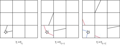
Figure 2: Illustration of rays propagating through the distributed computational domain at three time-steps $t_{i},t_{i+1}$, and $t_{i+2}$. To simplify the illustration, a box domain decomposition strategy is shown, where each square resembles one sub-domain. Further we assume that the source only emits two rays per time-step. The rays are propagated to the edges of each sub-domain during one time step. Then they are passed on to the neighbouring sub-domain to be processed in the next time step.

Propagation is thus delayed and a ray needs at most $\approx 2(N_{\rm{CPU}})^{1/3}$ time steps to pass through the box (assuming equipartition). The delay with which a ray is propagated through the box depends on the size of the time-step and the number of cores used. The larger the time-step is, the bigger the delay. The same applies for the number of cores.

If the crossing time of a ray in this scheme is well below the physical crossing time, the instant propagation approximation is considered retained. However rays will have differing propagation speeds from sub-domain to sub-domain. In the worst case scenario a ray only passes through one cell of a sub-domain. Therefore the minimal propagation speed is $v_{\rm{prop,min}}\approx 0.56\Delta l/\Delta t$, where $\Delta l$ is the size of one cell, $\Delta t$ the duration of one time step, and the factor 0.56 is the median distance of a randomly oriented ray passing through a cell of size unity as given in Ciardi et al. (2001). If the propagation speed of a packet is $v_{\rm{prop,min}}\gg c$, the propagation can be considered instantaneous, as in the original CRASH2. Even if this condition is not fulfilled and $v_{\rm{prop,min}}<c$, the resulting ionisation front and its evolution can still be correctly modelled (Gnedin & Abel, 2001), if the light crossing time is smaller than the ionisation timescale, i.e. when the ionisation front propagates at velocities much smaller than the speed of light. However the possibility exists, that near to a source, the ionisation timescale is shorter than the crossing time, resulting in the ionisation front to propagate at speeds artificially larger than light (Abel et al., 1999). With the segmented propagation scheme it has thus to be assured that the simulation parameters are chosen in such a way that the light crossing time is always smaller than the ionisation time scale.

The adopted parallelisation scheme can only be efficient, if the communication bandwidth per time step is saturated. Each time two cores need to communicate, there is a fixed overhead needed for negotiating the communication. If the information that is transferred in one communication event is small, the fixed overhead will dominate the communication scheme. It is therefore important to make sure that enough information is transferred per communication event for the overhead not to dominate the communication scheme. The original CRASH2 scheme only allowed for the propagation of one photon packet per source and time-step. In order to avoid the problem described above, this restriction has been relaxed and each source emits multiple photon packets per time step (Partl et al., 2010). Therefore in addition to the total number of photon packet produced per source $N_{\rm p}$ a new simulation parameter governing the total number of time steps $N_{\rm{t}}$ is introduced. The number of packets emitted by a source in one time step is thus $N_{\rm p}/N_{\rm{t}}$.

As in CRASH2, the choice of the global time step should not exceed the smallest of the following characteristic time scales: ionisation time scale, recombination time scale, collisional ionisation time scale, and the cooling time scale. If this condition is not met, the integration of the ionisation network and the thermal evolution is sub-sampled.

3.3 Parallel pseudo-random number generators

Since CRASH2 relies heavily on a pseudo-random numbers generator, here we have to face the challenging issue of generating pseudo-random numbers on multiple CPUs. Each CPU needs to use a different stream of random numbers with equal statistical properties. However this can be limited by the number of available optimal seeding numbers. A large collection of parallel pseudo random number generators is available in the SPRNG library (Mascagni & Srinivasan, 2000). From the library we are using the Modified Lagged Fibonacci Generator, since it provides a huge number of parallel streams (in the default setting of SPRNG $\approx 2^{39648}$), a large period of $\approx 2^{1310}$, and good quality random numbers. On top each stream returns a distinct sequence of numbers and not just a subset of a larger sequence.

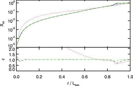
Figure 3: Test 0: Convergence study varying the number of photon packets $N_{\rm{p}}=10^{6},10^{7},10^{8},10^{9}$ used to simulate the evolution of an H ii region. Shown are the spherically averaged neutral hydrogen fraction profiles of the sphere as a function of radius at the end of the simulation. The dotted red line gives $N_{\rm{p}}=10^{6}$, the blue dashed line $N_{\rm{p}}=10^{7}$, the green dash dotted line $N_{\rm{p}}=10^{8}$, and the black solid line $N_{\rm{p}}=10^{9}$. The test used 8 CPUs. The lower panel shows the relative deviation $\epsilon$ of the pCRASH2 run from the highest resolution run.

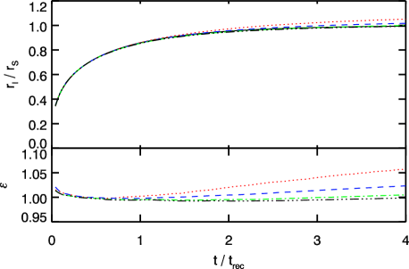
Figure 4: Test 0: Evolution of the H ii region’s size as a function of time normalised to the recombination time. The upper panel shows results for the convergence study where the number of photon packets was varied. The dotted red line gives $N_{\rm{p}}=10^{6}$, the blue dashed line $N_{\rm{p}}=10^{7}$, the green dash dotted line $N_{\rm{p}}=10^{8}$, and the black dash triple-dotted line $N_{\rm{p}}=10^{9}$. The solid black curve represents the analytic evolution $r_{S}(t)$. The test used 8 CPUs. The lower panel shows the relative deviation $\epsilon$ of the pCRASH2 runs from the analytic expression.

4 Performance

In this Section we present the results of an extensive comparison of the parallel scheme with the serial one. We follow the tests described in Maselli et al. (2003) and Iliev et al. (2006). Subsequently we discuss the speed performance of the parallel code and its scaling properties.

4.1 Test 0: Convergence test of a pure-H isothermal sphere

First we study the convergence behaviour of a Strömgren sphere as a function of the number of photon packets $N_{\rm{p}}$ and the number of time steps $N_{\rm{t}}$. The setup of this test is equivalent to Test 1 in the code comparison project (Iliev et al., 2006). For this test, we distribute the computational domain over 8 CPUs.

The time evolution of an H ii region produced by a source having a $10^{5}\textrm{ K}$ black-body spectrum with constant intensity expanding in a homogeneous medium is followed. The hydrogen density of the homogeneous medium is fixed at $n_{\rm{H}}=10^{-3}\textrm{ cm}^{-3}$, with no helium included. The temperature is fixed at $T=10^{4}\textrm{ K}$ and kept constant throughout the calculation. The initial ionisation fraction is initialised with $x_{{\mathbf{H\,\text{{ii}}}}}=1.2\times 10^{-3}$. The grid has a linear size of $L_{\rm{box}}=6.6\textrm{ kpc }h^{-1}$ and is composed of $N_{c}^{3}=128^{3}$ cells. The ionising source produces $\dot{N}_{\gamma}=5\times 10^{48}\textrm{ photons s}^{-1}$. Recombination radiation is followed and photons are emitted whenever 10% of the electrons in a cell have recombined. The simulation time is set at $t_{s}=5\times 10^{8}\textrm{ yr}$ which is approximately four times the recombination timescale.

In Fig. 3 we present the resulting spherically averaged profile of the neutral hydrogen fraction where we use $N_{\rm{p}}=10^{6},10^{7},10^{8},10^{9}$ photon packets. The number of time steps $N_{\rm{t}}$ is equal to the number of packets in order to obtain the identical scheme used in the serial version of CRASH2. $N_{\rm{p}}=10^{6}$ packets are unable to reproduce the correct neutral hydrogen fraction profile. Using $N_{\rm{p}}=10^{7}$ packets instead already yields satisfactory results, however we consider the solution to have converged with at least $N_{\rm{p}}=10^{8}$ packets. For this case the mean relative deviation $\left\langle\epsilon(r)\right\rangle=\left\langle x_{{\mathbf{H\,\text{{i}}}}}(r)/x_{{\mathbf{H\,\text{{i}}}},\mathrm{ref}}(r)\right\rangle$ of the neutral fraction to the $N_{\rm{p}}=10^{9}$ run is $0.7\%$. The largest relative deviation is found in a small region in the ionisation front itself. Its width is sensitive to the sampling resolution, where the solution for the $N_{\rm{p}}=10^{8}$ run differs by $18\%$ from the $N_{\rm{p}}=10^{9}$ run. In Fig. 4 the time evolution of the H ii region’s size is given. The radius is calculated using the volume of the H ii region, which is determined with $V=\sum_{\mathrm{cells}}x_{{\mathbf{H\,\text{{ii}}}},i}(\Delta l)^{3}$, where $\Delta l$ denotes the physical width of one cell. pCRASH2 is able to resolve the time evolution of the H ii region up to $2.5\%$ accuracy for $N_{\rm{p}}=10^{7}$ when compared with the analytic expression $r_{\mathrm{I}}(t)=r_{\mathrm{S}}\left(1-\exp(-t/t_{\mathrm{rec}})\right)$, where $t_{\mathrm{rec}}$ is the recombination time. Deviations from the analytic solution at $4t_{\mathrm{rec}}$ decrease to 0.5% for $N_{\rm{p}}=10^{8}$ and $0.2\%$ for $N_{\rm{p}}=10^{9}$. Because of these findings, we use $N_{\rm{p}}=10^{9}$ photon packets whenever the serial version allows for such a high sampling resolution, otherwise $N_{\rm{p}}=10^{8}$ packets will be used. We further note that the impact of the sampling resolution on the structure of the ionisation front is very important when the formation and destruction of molecular hydrogen is considered. It can significantly affect the stability of the ionisation front in cosmological simulations, in particular by introducing inhomogeneities in the star formation (Ricotti et al., 2002; Susa & Umemura, 2006; Ahn & Shapiro, 2007).

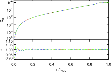
Figure 5: Test 0: Convergence study varying the number of time steps used to simulate the evolution of an H ii region. Shown are the spherically averaged neutral hydrogen fraction profile of the sphere as a function of radius at the end of the simulation. The dotted red line gives the results using $N_{\rm{t}}=10^{5}$ time steps, the blue dashed one $N_{\rm{t}}=10^{6}$ time steps, the green dash dotted one $N_{\rm{t}}=10^{7}$, and the black solid line $N_{\rm{t}}=10^{8}$ time steps. A constant number of $N_{\rm{p}}=10^{8}$ has been used. The test was run on 8 CPUs. The lower panel shows the relative deviation $\epsilon$ of the pCRASH2 run from the highest time resolution run.

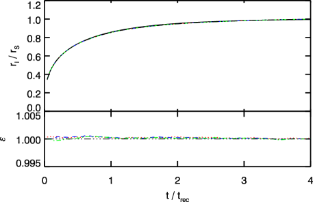
Figure 6: Test 0: Evolution of the H ii region’s size as a function of time normalised to the recombination time. The upper panel shows results for the convergence study where the number of time steps used in the simulation was varied. The number of packets used was fixed at $N_{\rm{p}}=10^{8}$. The dotted red line gives the results using $N_{\rm{t}}=10^{5}$ time steps, the blue dashed one $N_{\rm{t}}=10^{6}$ time steps, the green dash dotted one $N_{\rm{t}}=10^{7}$, and the black dashed triple-dotted line $N_{\rm{t}}=10^{8}$ time steps. The solid black curve represents the analytic evolution $r_{S}(t)$. The lower panel shows the relative deviation $\epsilon$ of the pCRASH2 runs from the solution using $N_{\rm{t}}=10^{8}$ time steps.

For the test where the number of time steps is varied (and thus the number of photons emitted per time step), we use $N_{\rm{p}}=10^{8}$ packets. The lower sampling resolution is used to reduce the accuracy with which the ionisation network is solved. Any influence of the time step length should be more easily seen if the accuracy in the solution of the ionisation network is lower. We evolve the H ii region using $N_{\rm{t}}=10^{5},10^{6},10^{7},10^{8}$ time steps. The resulting neutral hydrogen fraction profiles are given in Fig. 5. Overall, varying the number of time steps does not alter the resulting profile significantly. Only in the direct vicinity of the source, the solution is sensitive to the number of time steps used. In Fig. 6 the time evolution of the H ii region’s radius is shown for this test. The fluctuations between the results for various numbers of time steps are small, when compared to the $N_{\rm{t}}=10^{8}$. This is especially true for the equilibrium solution. At early times when the H ii region grows rapidly, the largest deviations can be seen. However for none of the cases the difference exceeds $0.05\%$. Since the choice of $N_{\rm{t}}$ directly determines the propagation speed of the photon packets, we confirm that the choice of propagation speed is not affecting the resulting H ii region and that the new ray propagation scheme is a valid approach.

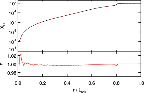
Figure 7: Test 1: Comparing the solvers of pCRASH2 with CRASH2. Shown are the spherically averaged neutral hydrogen fraction profile of the sphere as a function of radius at the end of the simulation. The red dotted line gives the pCRASH2 results and the black solid line the solution obtained with CRASH2. pCRASH2 was run on 8 CPUs. The lower panel shows the relative deviation $\epsilon$ of the pCRASH2 run from the serial CRASH2 run.

4.2 Comparing pCRASH2 with CRASH2

4.2.1 Test 1: Pure-H isothermal sphere

Now we compare the results obtained from pCRASH2 with those from the serial CRASH2 code. Since pCRASH2 evolves recombination radiation smoother (remember CRASH2 emits recombination photons at specific time steps while pCRASH2 emits diffuse radiation continuously), we expect differences between the two codes in regions where recombination radiation dominates. In order to show that pCRASH2’s solver performs identically to the one in CRASH2, we use the same setup as in Test 0, but we do not allow for recombination radiation to be emitted. For both codes, we set $N_{\rm{p}}=10^{9}$. The pCRASH2 solution is obtained on 8 CPUs, using $N_{\rm{t}}=10^{7}$ time steps.

The resulting neutral hydrogen fraction profile is shown in Fig. 7. The two curves of the CRASH2 and the pCRASH2 runs are barely distinguishable. The fluctuations in the relative deviations from the CRASH2 results near to the source are due to fluctuations in the least significant decimal. Only at the ionisation front, a small deviation of around 0.5% is seen. In the convergence study we have seen that the radial profile is sensitive to the sampling resolution at the ionisation front (IF) where the partially ionised medium abruptly turns into a completely neutral one. It is as well sensitive to the variance introduced by using different random number generator seeds. Tests using different seeds have shown, that fluctuations of up to $0.4\%$ between the various results can be seen. Therefore the small deviation in the ionisation front stems to some extent from the fact that pCRASH2 uses a different set of random numbers. The parallel solver thus gives results which are in agreement with the serial version. Including recombination radiation however will chance this picture, which we address with the next test.

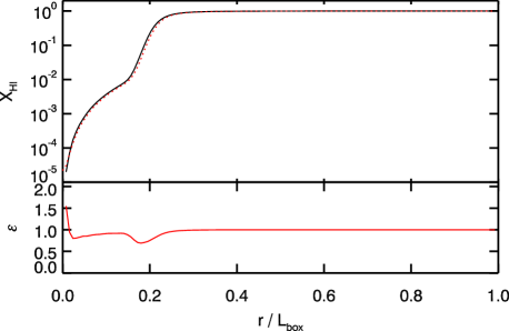
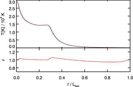
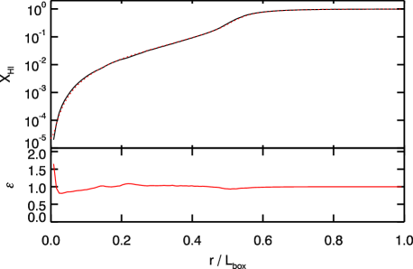
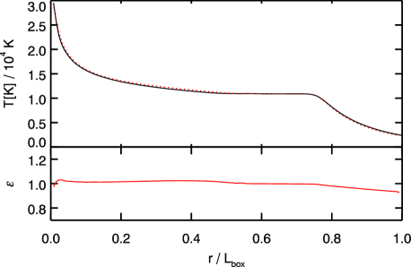
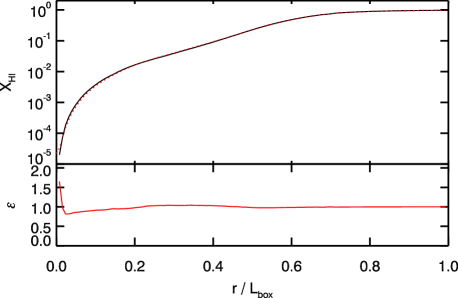
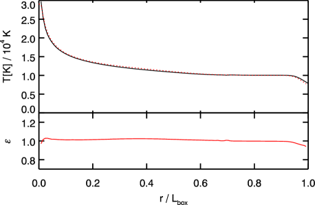
Figure 8: Test 2: Comparing the results of pCRASH2 (red dotted line) with CRASH2 (black line). Shown are the spherically averaged neutral hydrogen fraction profiles of the sphere as a function of radius (left column) and the temperature profiles (right column) at $t=1\times 10^{7},2\times 10^{8},5\times 10^{8}\textrm{ yr}$ (from top to bottom). The pCRASH2 results are obtained on 8 CPUs. The small bottom panels show the relative deviation from the CRASH2 reference solution.

4.2.2 Test 2: Realistic H ii region expansion.

The test we are now focusing on is identical to Test 2 in the radiative transfer codes comparison paper (Iliev et al., 2006), except that we use a larger box size to better accommodate the region preceding the ionisation front where preheating due to higher energy photons is important. We use the same setup as in Test 0, but now we follow the temperature evolution, and self-consistently account for the reemission. Again the gas is initially fully neutral. Its initial temperature however is now set to $T=100\textrm{ K}$. The source emits $N_{\rm{p}}=4\times 10^{9}$ photon packets. Again we compare the solution obtained with CRASH2 to the one obtained with pCRASH2, which for the present test is run with $N_{\rm{t}}=10^{7}$ time steps on 8 CPUs.

In Fig. 8 we show the resulting neutral hydrogen fraction profiles and temperature profiles at three different time steps $t=1\times 10^{7},2\times 10^{8},5\times 10^{8}\textrm{ yrs}$. Plotted are the solutions obtained with CRASH2 and with pCRASH2 (solid black and red dotted lines respectively). At $t=1\times 10^{7}\textrm{ yrs}$, the results of CRASH2 and pCRASH2 slightly differ at the ionisation front. The structure of the ionisation front appears slightly sharper in the pCRASH2 run, than in the CRASH2 run. In the front, recombination radiation is an important process (Ritzerveld, 2005). Since pCRASH2 continuously emits recombination photons whenever a cell reaches the recombination threshold and not only at fixed time steps, the diffuse field is better sampled and the ionisation front becomes sharper. For this test, CRASH2 sampled the diffuse field $10^{3}$ times through the whole simulation. In pCRASH2 the number of cell crossings determines the sampling resolution of the recombination radiation. Therefore recombination radiation originating in the cells of the ionisation front is evaluated at least $5\times 10^{4}$ times for this specific run. A higher sampling rate in the recombination radiation reproduces its spectral energy distribution which is strongly peaked towards the H i photo-ionisation threshold (see the Milne spectrum) more accurately, resulting in a sharper ionisation front. Better sampling of the Milne spectrum reproduces its shape more accurately and reduces the possibility that too much energy is deposited in the high energy tail of the Milne spectrum due to the poor sampling resolution of the spectrum.

At later times the two codes give similar results for the hydrogen ionisation fraction, with almost negligible differences close to the source and across the ionisation front. This is also seen in the temporal evolution of the H ii region’s radius given in Fig. 9, which is determined as described in Test 0. In the beginning the differences between the codes are at most $3\%$, decreasing steadily up to one recombination time. This clearly shows the effect of the smooth emission of recombination radiation in pCRASH2. After one recombination time, the differences between the two codes are small and convergence is achieved. A similar picture emerges for the temperature profile. As for the ionisation front, the preceding temperature front is as well slightly sharper with pCRASH2.

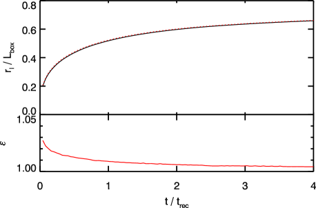
Figure 9: Test 2: Comparing the time evolution of the H ii region’s radius from the pCRASH2 run (red dotted line) with CRASH2 (black line). The pCRASH2 results are obtained on 8 CPUs. The small bottom panel show the relative deviation from the CRASH2 reference solution.

4.2.3 Test 3: Realistic H ii expansion in a H+He medium

In this test, we study the expansion of an H ii region in a medium composed of hydrogen and helium. This corresponds to the CLOUDY94 test in Maselli et al. (2009). We consider the H ii region produced by a $T=6\times 10^{4}\textrm{ K}$ blackbody radiator with a luminosity of $L=10^{38}\textrm{ erg s}^{-1}$. The point source ionises a uniform medium with a density of $n=1\textrm{ cm}^{-3}$ in a gas composed of 90% hydrogen number density and the rest helium. The temperature is initially set at $T=10^{2}\textrm{ K}$ and its evolution is solved for. The dimension of the box is $L_{\mathrm{box}}=128\textrm{ pc}$. The test is run for $t_{s}=6\times 10^{5}\textrm{ yrs}$ after which ionisation equilibrium is reached with $N_{\rm{p}}=2\times 10^{8}$. pCRASH2 was run on 8 CPUs with $N_{\rm{t}}=10^{8}$.

In Fig. 10 we compare the resulting temperature, hydrogen and helium density profiles from pCRASH2 with the ones obtained with CRASH2. Overall the resulting pCRASH2 profiles are in good agreement with CRASH2. Again only slight deviations from the CRASH2 solution are present in the outer parts of the H ii region due to higher sampling resolution of the ionising radiation re-emitted in recombinations. As in the previous test, the pCRASH2 solution shows somewhat sharper fronts in hydrogen and temperature. The hydrogen fronts are shifted slightly further away from the source in pCRASH2, giving rise to the large relative error. Otherwise pCRASH2’s performance is equivalent to that of CRASH2.

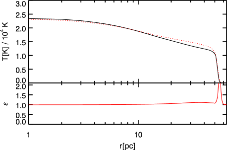
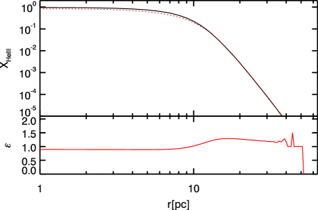
Figure 10: Test 3: Realistic H ii region extending in a hydrogen + helium medium. Compared are equilibrium results obtained with CRASH2 (black solid line) to ones obtained with pCRASH2 (red dotted line). The upper left panel gives the profile of neutral hydrogen fractions, lower left panel gives singly ionised helium fractions, and the lower right panel gives the double ionised helium fractions. The upper right panel gives the spherically averaged temperature profile as a function of radius.The small bottom panels show the relative deviation of the pCRASH2 run from the CRASH2 reference solution.

4.2.4 Test 4: Multiple sources in a cosmological density field

The setup of this test is identical to Test 4 in the radiative transfer codes comparison paper (Iliev et al., 2006). Here the formation of H ii regions from multiple sources is followed in a static cosmological density field at redshift $z=9$, including photo-heating. The initial temperature is set to $T=100\textrm{ K}$. The positions of the 16 most massive halos are chosen to host $10^{5}\textrm{ K}$ black-body radiating sources. Their luminosity is set to be proportional to the corresponding halo mass and all sources are assumed to switch on at the same time. No periodic boundary conditions are used. The ionisation fronts are evolved for $t_{s}=4\times 10^{7}\textrm{ yr}$. Each source produces $N_{\rm{p}}=1\times 10^{7}$ photon packets. pCRASH2 is run with $N_{\rm{t}}=10^{6}$ time steps on 16 CPUs.

A comparison between slices of the neutral hydrogen fraction and the temperatures obtained with pCRASH2 and CRASH2 are given in Fig. 11 for $t=0.05\textrm{ Myr}$ and Fig. 12 for $t=0.2\textrm{ Myr}$. For both time steps the pCRASH2 results produce qualitatively similar structures compared to CRASH2 in the neutral fraction and temperature fields. Slight differences however are present, mainly in the vicinity of the ionisation fronts, due to the differences in how recombination is treated, as already discussed. In the lower panels of the same figures we show also the probability distribution functions for the hydrogen neutral fractions and the temperatures. Here the differences are more evident. The neutral fractions obtained with pCRASH2 do not show strong deviations from the CRASH2 solution. In the distribution of temperatures however, pCRASH2 tends to heat up the initially cold regions somewhat faster than CRASH2, as can be seen by the 20% drop in probability for the $t=0.05\textrm{ Myr}$ time step at low temperatures. This can be explained by the fact that the dominant component to the ionising radiation field in the outer parts of H ii regions is given by the radiation emitted in recombinations. The better resolution adopted in pCRASH2 for the diffuse field is then responsible for slightly larger H ii regions. Since a larger volume is ionised and thus hot, the fraction of cold gas is smaller in the pCRASH2 run, than in the reference run. At higher temperatures however, the distribution functions match each other well. Only in the highest bin a discrepancy between the two code’s solutions can be noticed, but given that there are at most four cells contributing to that bin, this is consistent with Poissonian fluctuations.

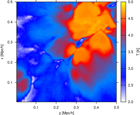
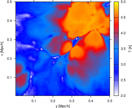
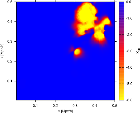
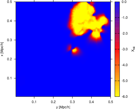
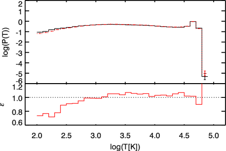
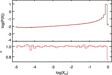
Figure 11: Test 4: Cut through the temperature fields (upper panels) and neutral hydrogen fractions (middle panels) at time-step $t=0.05\textrm{ Myr}$. Left panels show the solution obtained with CRASH2, right panels show the pCRASH2 solution. The lower panels give volume weighted temperature and neutral fraction probability distribution functions obtained with CRASH2 (black) and pCRASH2 (red dotted), where the error bars give Poissonian errors. The small bottom panels show the relative deviation of the pCRASH2 run from the CRASH2 reference solution.

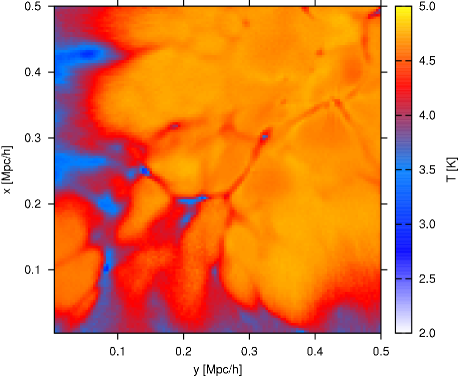
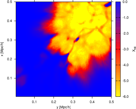
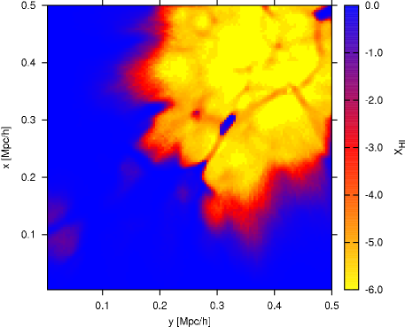
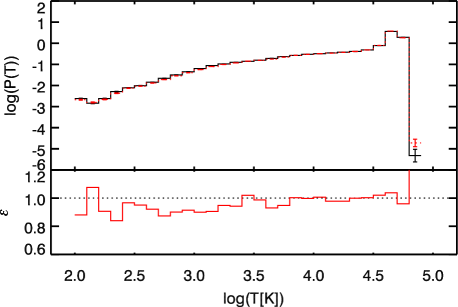
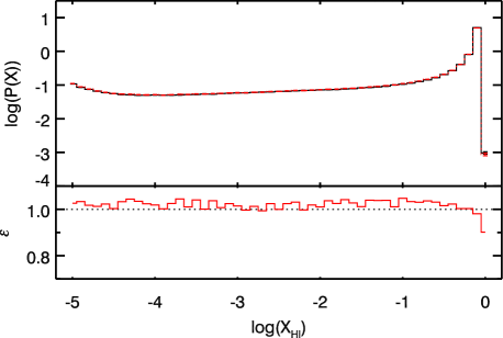
Figure 12: Test 4: Same as in Fig. 11 at time-step $t=0.2\textrm{ Myr}$.

4.3 Scaling properties

By studying the weak and strong scaling properties of a code, it is possible to assess how well a problem maps to a distributed computing environment and how much speed increase is to be expected from the parallelisation. Strong scaling describes the scalability by keeping the overall problem size fixed. Weak scaling on the other hand refers to how the scalability behaves when only the problem size per core is kept constant (i.e. the fraction between the total problem size and the number of CPUs stays constant).

We will use the test cases described above, to study the impact of the various input parameters such as grid size, number of photon packets, number of sources, and type of physics used, on the scalability. Scalability is measured with the speed up, which is defined as the execution time on a single core divided by the execution time on multiple cores. Due to the long simulation times of our test cases on a single core (for some test cases of the order of weeks), the execution time on a single core was only determined once. This certainly makes our normalisation point subject to variance, which has to be taken into account in the following discussion. All results presented in this section have been obtained on a cluster at the Astrophysikalisches Institut Potsdam (AIP) with computational nodes consisting of two Intel Xeon Quad Core 2.33GHz processors each. Since our parallelisation scheme has shortly spaced communication points, very good communication latency is required, which on our system is guaranteed through an InfiniBand network.

4.3.1 Test 2

Achieving good scaling for Test 2 is a challenge, since only one source sits in a corner of the box and a strong load imbalance between the sub-domains near to the source and the ones further away exists. The fact that the gas is initially neutral even intensifies the imbalance, since at first the domains far away from the source will be idle. Only as the H ii region grows, more and more sub-domains will be involved in the calculation. This test is therefore a good proxy for how the code scales in extreme situations and shows the strong scaling relation for one source. In Fig. 13 we show the results obtained with the setup described above. In principle it is expected, that the more rays each domain has to process in one time-step, the better the scaling becomes. Therefore we run the test once without recombination emission and once with. Further we increased the grid size to $256^{3}$ and $512^{3}$ cells, which increases the amount of calculations needed per sub-domain. This yields the weak scaling properties for one source as a function of grid size.

The scaling relation is mainly determined by Ahmdal’s law (Amdahl, 1967), which relates the parallelised parts of a code (in our case the propagation of photons) with the unparallelised parts (such as communication between sub-domains). It states that the maximum possible speed up is solely limited by the fraction of time spent in serial parts of the code. The scaling relation behaves for all runs similarly. An almost linear speedup is achieved up to 8 CPUs per node, and a deviation from linear scaling according to Ahmdal’s law arises when communication over the network is needed. The deviation is dependent on the amount of work to be processed per time-step.

In the worst case of a $128^{3}$ celled grid without reemission, the deviation is the largest. Following recombination emission and thus increasing the workload yields better scaling up to the point where one computational node is saturated. For one source the best scaling is achieved with larger grid sizes. For the $512^{3}$ grid it is even reasonable to use 16 CPUs on two nodes on our cluster and allow for communication of rays over the network. However with 32 CPUs, 50% of the computational resources remain unused.

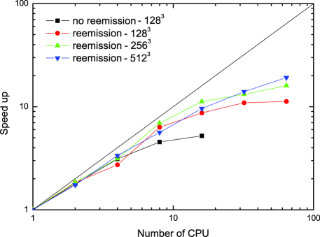
Figure 13: Speed up achieved on our local cluster for Test 2 as a function of grid-size and number of CPUs. The straight black line indicates a linear ideal scaling property.

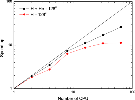
Figure 14: Test3: Scaling relation of the Cloudy test case as a function of number of CPUs. For comparison, the results of the hydrogen only Test 2 are given as red line.

4.3.2 Test 3

Up to now, we have only considered the gas to be made up solely of hydrogen. We now study the scaling properties of one source embedded in gas made of a mixture of hydrogen and helium. Now each domain needs to solve a more complicated set of equations and more time is spent in solving the chemical-thermal equations network than in propagating photons. The ionisation network needs to track the two additional species introduced with helium, plus the related contribution to heating and cooling which enters the temperature calculation. Since solving the ionisation-thermal network is the most computationally expensive part of our algorithm, the additional work results in an approximate increase of overall execution time by a factor of three or more. Furthermore recombining helium will produce additional photons that need to be followed, even further increasing the computational load. As the communication demand stays the same as in Test 2, the scaling relation is expected to be better than in the hydrogen only case. In Fig. 14 we present the scaling performance obtained with the Cloudy test case described above using $N_{\rm{p}}=2\times 10^{9}$ photon packets and $N_{\rm{t}}=10^{7}$ time-steps. Comparing the scaling with the one achieved in Test 2, it is evident, that solving more detailed physics improves scaling. Now for the Cloudy test, ideal scaling is achieved as long as the problem is confined to one node (in our case 8 CPU) and no information needs to be communicated over the network. However the fact that more time is spend in solving the rate equations, communication latency across the network does not affect scaling as strongly as in Test 2. It now even makes sense to use 32 CPUs for one source, yielding a speed up of around 16. As a comparison Test 2 achieved a speed up of around 10 for 32 CPUs.

As a final check we have also run a set of simulations for Test 3 with an increased gas density, $n_{H}=10$ cm^-3, all the other quantities being the same. The aim of this experiment is to test the scaling under conditions in which diffuse radiation from recombinations becomes important. Somewhat to our surprise, we do not find any appreciable differences in the scaling relation between the low- and high-density cases. However, this can be easily understood as follows: The simulation time is set at five times the recombination time. Hence the same amount of recombinations per time step occur (when normalised to the density of the gas) in both runs. Since recombination photons are produced when a certain fraction of the gas has recombined, the number of emitted recombination photons is similar in the two runs. Therefore the amount of CPU time spent in the diffuse component is similar and the scaling does not change.

4.3.3 Test 4

By studying the scaling properties of Test 4, we can infer how the code scales with increasing number of sources. Since Test 4 uses an output of a cosmological simulation, the sources are not distributed homogeneously in the domain. Therefore large portions of the grid remain neutral as is seen in Fig. 12. This poses a challenge to our domain decomposition strategy and might deteriorate scalability.

First we study the scaling of the original Test 4, with a sample of $10^{8}$ photon packets emitted by each of the 16 sources. Then we increase the number of photons per source to $10^{9}$. Since large volumes remain neutral, we further study an idealised case, where the whole box is kept highly ionised by initialising every cell to be 99% ionised. The results of these experiments are shown in Fig. 15. In the case of only $10^{8}$ photon packets per source, good scaling can only be reached up to 8 CPUs (i.e. a single node), as was the case with only one source. Communication over the network cannot be saturated with such a small number of photons and its overhead is larger than the time spent in computations. However by increasing the number of samples per time-step improves scaling. In the idealised optically thin case, perfect scaling is reached even up to 16 CPUs and starts to degrade for higher numbers of CPU. The discrepancy between the neutral and fully ionised case shows the influence of load imbalance due to the large volumes of remaining neutral gas.

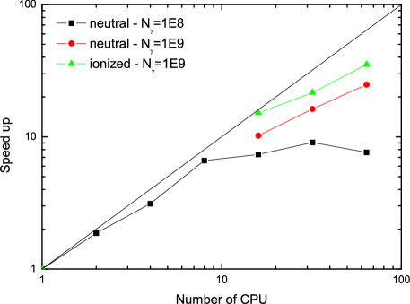
Figure 15: Scaling achieved with Test 4 as a function of number of photon, optically thickness and number of CPUs.

Since good scaling was found in the original Test 4, we now increase the number of sources. For this we duplicate the sources in Test 4, and mirror their position at an arbitrary axis. This preserves the clustered nature of the sources, while distributing them throughout the computational volume. With this prescription we increase the number of sources to 32 and 64. Again each source emits $10^{9}$ photon packets and the idealised case of an optically thin box is studied. The results of the speed up function are given in Fig. 16. As expected, the more computational intensive the problem becomes, the better the scaling. In the figure, the speed up for the 64 sources lies below the others cases because we have linearly extrapolated the normalisation point of the 32 sources run to the 64 sources case, since the time to run the simulation on one CPU was too long. This of course is just a rough estimate, and in fact it is responsible for the lower speed up values. Despite of it, the trend still gives a measure of the improved scaling with respect to the cases with 32 and 16 sources. While a difference in the speed up between the three test-cases is seen when increasing from 1 to 16 CPUs, it is difficult to tell whether this is a genuine feature of our parallelisation strategy or just a manifestation of the variance in the normalisation.

Figure 16: Scaling achieved with Test 4 as a function of number of sources and number of CPUs for an ideal optically thin case.

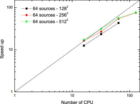
Figure 17: Scaling relation of Test 4 as a function of box size with 64 sources and number of CPUs for an ideal optically thin case.

Up to now we have only considered the case of a $128^{3}$ box. We now re-map the density field of Test 4 to $256^{3}$ and $512^{3}$ grids. The resulting scaling properties for the ideal optically thin case with 64 sources are presented in Fig. 17. The scaling properties are not dependent on the size of the grid, and weak scaling only exists as long as the number of cores does not exceed the number of sources.

We can thus conclude that our parallelisation strategy shows perfect weak scaling properties when increasing the numbers of sources (compare Fig. 16). Increasing the size of the grid does not affect scaling. However weak scaling in terms of the grid size only works as long as the number of CPUs does not exceed the number of sources (see Fig. 17 going from 64 to 128 CPUs).

From these tests, we can formulate an optimal choice for the simulation setup. We have seen that better scaling is achieved with large grids. Further linear scaling can be achieved in the optically thin case by using up to as may cores as there are sources. For the optically thick case however, deterioration of the scaling properties needs to be taken into account.

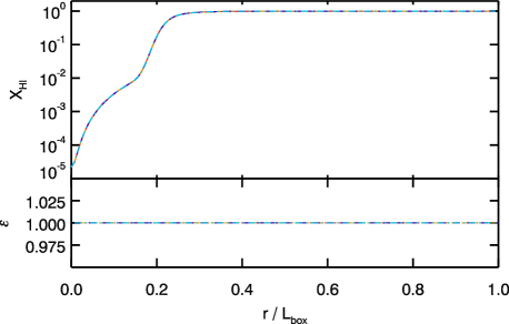
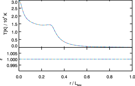
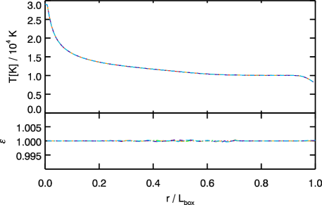
Figure 18: Test 2: Dependence of the solution on the number of cores. The large upper panels show the results of pCRASH2 obtained on 1 CPU (red dotted line), 2 CPUs (blue dashed line), 4 CPUs (green dash dotted line), 8 CPUs (orange dash dot dotted line), 16 CPUs (violet dashed line), and 32 CPUs (light blue dash dotted line). The results are compared with the CRASH2 solution (black solid line). Shown are the spherically averaged neutral hydrogen fraction profiles of the sphere as a function of radius (left column) and the temperature profiles (right column) at $t=1\times 10^{7}$ (top), and $5\times 10^{8}\textrm{ yr}$ (bottom). The small bottom panels show the relative deviation from the single CPU pCRASH2 solution.

4.4 Dependence of the solution on the number of cores

Since each core has its own set of random numbers, the solutions of the same problem obtained with different numbers of cores will not be identical. They will vary according to the variance introduced by the Monte Carlo sampling. To illustrate the effect, we revisit the results of Test 2 and study how the number of cores used to solve the problem affects the solution.

The results of this experiment are shown in Fig. 18, where we compare the different solutions obtained with various numbers of CPUs. Solely by looking at the profiles, no obvious difference between the runs can be seen. Variations can only be seen in the relative differences of the various runs which are compared with the single CPU pCRASH2 run.

At $t=10^{7}\textrm{ yr}$ the runs do not show any differences. In Sec. 4.2.2 we have seen, that recombination radiation has not yet started to be important. This is exactly the reason why, at this stage of the simulation, no variance has developed between the different runs. Since the source is always handled by the first core and the set of random number is always the same on this core no matter how many CPUs are used, the results are always identical. However as soon as the Monte Carlo sampling process start to occur on multiple nodes, the set of random numbers starts to deviate from the single CPU run and variance in the sampling is introduced. At the end of the simulation at $t=5\times 10^{8}\textrm{ yr}$, large parts of the H ii region are affected by the diffuse recombination field and variance between the different runs is expected. By looking at Fig. 18, the Monte Carlo variance for the neutral hydrogen fraction profile lies between 1% and 2%. The temperature profile is not as sensitive to variance as the neutral hydrogen fraction profile. For the temperature the variance lies at around 0.1%.

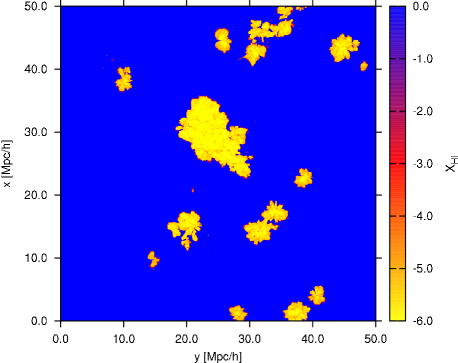
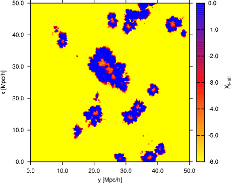
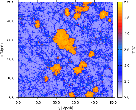
Figure 19: Cut through a cosmological simulation at $z=8.3$ with the neutral hydrogen fraction field (upper left panel), the singly ionised helium fraction (upper right panel), the doubly ionised helium fraction (lower left panel), and the temperature field (lower right panel) at time-step $t=1\times 10^{6}\textrm{ yr}$ using 1000 sources.

4.5 Thousand sources in a large cosmological density field

Up to now we have discussed pCRASH2’s performance with controlled test cases. We now demonstrate pCRASH2’s ability to handle large highly resolved cosmological density fields embedding thousands of sources. We utilise the $z=8.3$ output of the MareNostrum High-z Universe (Forero-Romero et al., 2010) which is a $50\textrm{ Mpc }h^{-1}$ SPH simulation using $2\times 1024^{3}$ particles equally divided into dark matter and gas particles. The gas density and internal energy are assigned to a $512^{3}$ grid using the SPH smoothing kernel. A hydrogen mass fraction of $76\%$ and a helium mass fraction of $24\%$ are assumed.

The UV emitting sources are determined similarly to the procedure used in Test 4 of the comparison project (Iliev et al., 2006) by using the 1000 most massive haloes in the simulation. We evolve the radiation transport simulation for $10^{6}\textrm{ yr}$ and follow the hydrogen and helium ionisation, as well as photo-heating. Recombination emission is included. Each source emits $10^{8}$ photon packets in $10^{7}$ time steps. In total $10^{11}$ photon packets are evaluated, not counting recombination events. The simulation was run on a cluster using 16 nodes, with a total of 128 cores. The walltime for the run as reported by the queuing system was 143.5 hours; the serial version would have needed over two years to finish this simulation.

In Fig. 19 cuts through the resulting ionisation fraction fields and the temperature field are shown at $t=10^{6}\textrm{ yr}$. It can be clearly seen that the H ii regions produced by the different sources already overlap each other. Further the ionised regions strongly deviate from spherical symmetry. This is caused by the fact that the ionisation fronts propagate faster in underdense regions than in dense filaments.

The distribution of He ii follows the distribution of ionised hydrogen, except in the centre of the ionisation regions, where helium becomes doubly ionised and holes start to emerge in the He ii maps. Photo-heating increases the temperature in the ionised regions to temperatures of around $30000\textrm{ K}$.

These results are presented here as an example of highly interesting problems in cosmological studies which can be easily addressed with pCRASH2, but that would be impossible to handle with the serial version of the code CRASH2.

5 Summary

We have developed and presented pCRASH2, a new parallel version of the CRASH2 radiative transfer scheme code, whose description can be found in Maselli et al. (2003), Maselli et al. (2009) and references therein. The parallelisation strategy was developed to map the CRASH2 algorithm to distributed memory machines, using the MPI library.

In order to obtain an evenly load balanced parallel algorithm, we statically estimate the computational load in each cell by calculating the expected ray number density assuming an optically thin medium. The ray density in a cell is then inversely proportional to the distance to the source squared. Using the Peano-Hilbert space filling curve, the domain is cut into sub-domains; the integrated ray number density in the box is determined and equally divided by the number of processors. Then the expected ray number density is integrated along the curve and cut, whenever this fraction of the total ray number density is reached. The result of this is a well balanced domain decomposition, that even performs adequately in optically thick regimes.

For the parallelisation of the ray tracing itself, we have segmented the propagation of rays over multiple time steps. In the original CRASH2 implementation it was assumed that photons instantly propagate through the whole box in one time step. In pCRASH2 however rays are only propagated through one sub-domain per time step. After rays have propagated to the border of the sub-domain, they are then passed on to the neighbouring domain for further processing in the following time step. With this segmentation strategy we keep communication between the domains low and locally confined.

Since pCRASH2 is able to handle a larger amount of photon packets than the serial version, we have additionally increased the sampling resolution of the diffuse recombination radiation. With this parallelisation strategy, we obtain a high-performing algorithm, that scales well for large problem sizes. We have extensively tested pCRASH2 against a standardised set of test cases to validate the parallelisation scheme.

With pCRASH2 it is now possible to address a number of problems that require the tracking of the UV field produced by a large number of sources, that so far were not attainable for CRASH2 because of the high computational cost. A natural application is the evolution of the UV flux field, especially during the era of reionisation. The phase transition of the initially neutral H+He intergalactic to its fully ionised state can now be accurately followed in the large volumes required to achieve a good representation of the process on cosmological scales ($>300\textrm{Mpc}$).

On the other hand, pCRASH2 has a broader application range. In fact, it is not limited to tackle cosmological configurations, and can be applied to study a wealth of astrophysical problems, e.g. the propagation and impact of UV flux field in the vicinity of star forming galaxies, to mention one example. Finally, due to pCRASH2’s distributed memory approach, new physics such as extending the ionisation network to species other than hydrogen and helium can be now easily implemented.

Appendix A Generating the Peano-Hilbert curve

Space filling curves present an easy method to systematically reach every point in space and are usually fractal in nature. Various space filling curves such as the Peano curve, the Z-order, or the Peano-Hilbert curve exist. The most optimal in terms of clustering (i.e. that all points on the curve are spatially near to each other) is the Peano-Hilbert curve. We will now sketch the fast Peano-Hilbert algorithm used by the domain decomposition algorithm for projecting cells on the grid which is a subset of the natural numbers including zero $\mathbb{N}_{0}^{3}$ onto an array in $\mathbb{N}_{0}^{1}$. A detailed description of its implementation is found in Chenyang et al. (2008).

Let $H_{m}^{N}$, $(m\geq 1,N\geq 2)$ describe an $N$-dimensional Peano-Hilbert curve in its $m$th-generation. $H_{m}^{N}$ thus maps $\mathbb{N}_{0}^{N}$ to $\mathbb{N}_{0}^{1}$, where we call the mapped value in $\mathbb{N}_{0}^{1}$ a Hilbert-key. A $m$th-generation Peano-Hilbert curve of $N$-dimension is a curve that passes through a hypercube of $2^{m}\times\ldots\times 2^{m}=2^{mN}$ in $\mathbb{N}_{0}^{N}$. For our purpose we only consider $N\leq 3$.

Let the 1st-generation Peano-Hilbert curve be called a $N$-dimensional Hilbert cell $C^{N}$ (see Fig. 20 for $N=2$). In binary digits, the coordinates of the $C^{2}[\textrm{Hilbert-key}]$ Hilbert cell can be expressed as $C^{2}[0]=00$, $C^{2}[1]=01$, $C^{2}[2]=11$, and $C^{2}[3]=10$, where each binary digit represents one coordinate $X_{N}$ in $\mathbb{N}_{0}^{N}$ with the least significant bit at the end, i.e. $C^{2}[i]=X_{2}X_{1}$. For $N=3$ the Hilbert cell becomes $C^{3}[0]=000$, $C^{3}[1]=001$, $C^{3}[2]=011$, $C^{3}[3]=010$, $C^{3}[4]=110$, $C^{3}[5]=111$, $C^{3}[6]=101$, $C^{3}[7]=100$.

The basic idea in constructing an algorithm that maps $\mathbb{N}_{0}^{N}$ onto the $m$th-generation Peano-Hilbert curve is the following. Starting from the basic Hilbert cell, a set of coordinate transformations which we call Hilbert genes is applied $m$-times to the Hilbert cell and the final Hilbert-key is obtained. An illustration of this method is shown in Fig. 20. Here the method of extending the 1st-generation 2-dimensional Peano-Hilbert curve to the 2nd-generation is shown. Analysing the properties of the Peano-Hilbert curve reveals that two types of coordinate transformations operating on the Hilbert cell are needed for its construction. The exchange of coordinates and the reverse operation. The exchange operation $X_{2}\leftrightarrow X_{3}$ on $011$ would result in $101$. The reverse operation denotes a bit-by-bit reverse (e.g. reverse $X_{1},X_{3}$ on $010$ results in $111$). Using these transformations and the fact, that the $m$th-generation Hilbert-key can be extended or reduced to an $(m+1)$- or $(m-1)$th-generation Hilbert-key by bit-shifting the key by $N$ bits up or down, the Hilbert-key can be constructed solely using binary operations.

For the $N=2$ case illustrated in Fig. 20 the Hilbert genes $G^{N}[\textrm{Hilbert-key}]$ are the following: $G^{2}[0]=$ exchange $X_{1}$ and $X_{2}$, $G^{2}[1]=$ no transformation, $G^{2}[2]=$ no transformation, and $G^{2}[3]=$ exchange $X_{1}$ and $X_{2}$ plus reverse $X_{1}$ and $X_{2}$. Through repeated application of these transformations on the $m$th-generation curve, the $(m+1)$th-generation can be found.

The Hilbert genes for $N=3$ are: $G^{3}[0]=$ exchange $X_{1}$ and $X_{3}$, $G^{3}[1]=$ exchange $X_{2}$ and $X_{3}$, $G^{3}[2]=$ no transformation, $G^{3}[3]=$ exchange $X_{1}$ and $X_{3}$ plus reverse $X_{1}$ and $X_{3}$, $G^{3}[4]=$ exchange $X_{1}$ and $X_{3}$, $G^{3}[5]=$ no transformation, $G^{3}[6]=$ exchange $X_{2}$ and $X_{3}$ plus reverse $X_{2}$ and $X_{3}$, and $G^{3}[7]=$ exchange $X_{1}$ and $X_{3}$ plus reverse $X_{1}$ and $X_{3}$.

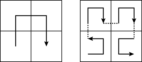
Figure 20: Left panel: The Hilbert cell $C^{2}\equiv H_{1}^{2}$ for $N=2$. Right panel: Applying the $N=2$ Hilbert genes on the Hilbert cell produces the 2nd-generation Peano-Hilbert curve.

References

- Abel et al. (1999) Abel T., Norman M. L., Madau P., 1999, ApJ, 523, 66
- Abel & Wandelt (2002) Abel T., Wandelt B. D., 2002, MNRAS, 330, L53
- Ahn & Shapiro (2007) Ahn K., Shapiro P. R., 2007, MNRAS, 375, 881
- Alme et al. (2001) Alme H. J., Rodrigue G. H., Zimmerman G. B., 2001, The Journal of Supercomputing, 18, 5
- Amdahl (1967) Amdahl G. M., 1967, in AFIPS ’67 (Spring): Proceedings of the April 18-20, 1967, spring joint computer conference Validity of the single processor approach to achieving large scale computing capabilities. ACM, New York, NY, USA, pp 483–485
- Baek et al. (2009) Baek S., Di Matteo P., Semelin B., Combes F., Revaz Y., 2009, A&A, 495, 389
- Bianchi et al. (1996) Bianchi S., Ferrara A., Giovanardi C., 1996, ApJ, 465, 127
- Chenyang et al. (2008) Chenyang L., Hong Z., Nengchao W., 2008, Computational Science and its Applications, International Conference, 0, 507
- Ciardi et al. (2001) Ciardi B., Ferrara A., Marri S., Raimondo G., 2001, MNRAS, 324, 381
- Forero-Romero et al. (2010) Forero-Romero J. E., Yepes G., Gottlöber S., Knollmann S. R., Khalatyan A., Cuesta A. J., Prada F., 2010, MNRAS, 403, L31
- Gnedin & Abel (2001) Gnedin N. Y., Abel T., 2001, New Astronomy, 6, 437
- Hasegawa & Umemura (2010) Hasegawa K., Umemura M., 2010, ArXiv e-prints
- Iliev et al. (2006) Iliev I., Ciardi B., Alvarez M., Maselli A., Ferrara A., Gnedin N., Mellema G., Nakamoto T., Norman M., Razoumov A., Rijkhorst E.-J., Ritzerveld J., Shapiro P., Susa H., Umemura M., Whalen D., 2006, Mon. Not. R. Astron. Soc., 371, 1057
- Iliev et al. (2006) Iliev I. T., Mellema G., Pen U., Merz H., Shapiro P. R., Alvarez M. A., 2006, MNRAS, 369, 1625
- Iliev et al. (2009) Iliev I. T., Whalen D., Mellema G., Ahn K., Baek S., Gnedin N. Y., Kravtsov A. V., Norman M., Raicevic M., Reynolds D. R., Sato D., Shapiro P. R., Semelin B., Smidt J., Susa H., Theuns T., Umemura M., 2009, MNRAS, 400, 1283
- Jonsson (2006) Jonsson P., 2006, MNRAS, 372, 2
- Juvela (2005) Juvela M., 2005, A&A, 440, 531
- Knollmann & Knebe (2009) Knollmann S. R., Knebe A., 2009, ApJS, 182, 608
- Marakis et al. (2001) Marakis J., Chamico J., Brenner G., Durst F., 2001, International Journal of Numerical Methods for Heat & Fluid Flow, 11, 663
- Mascagni & Srinivasan (2000) Mascagni M., Srinivasan A., 2000, ACM Trans. Math. Softw., 26, 436
- Maselli et al. (2009) Maselli A., Ciardi B., Kanekar A., 2009, MNRAS, 393, 171
- Maselli & Ferrara (2005) Maselli A., Ferrara A., 2005, MNRAS, 364, 1429
- Maselli et al. (2003) Maselli A., Ferrara A., Ciardi B., 2003, MNRAS, 345, 379
- McQuinn et al. (2007) McQuinn M., Lidz A., Zahn O., Dutta S., Hernquist L., Zaldarriaga M., 2007, MNRAS, 377, 1043
- Mellema et al. (2006) Mellema G., Iliev I. T., Alvarez M. A., Shapiro P. R., 2006, New Astronomy, 11, 374
- Mihalas & Weibel Mihalas (1984) Mihalas D., Weibel Mihalas B., 1984, Foundations of radiation hydrodynamics
- Paardekooper et al. (2010) Paardekooper J., Kruip C. J. H., Icke V., 2010, A&A, 515, A79+
- Partl et al. (2010) Partl A. M., Dall’Aglio A., Müller V., Hensler G., 2010, ArXiv e-prints, arxiv:1009.3424
- Pawlik & Schaye (2008) Pawlik A. H., Schaye J., 2008, MNRAS, 389, 651
- Petkova & Springel (2009) Petkova M., Springel V., 2009, MNRAS, 396, 1383
- Razoumov et al. (2002) Razoumov A. O., Norman M. L., Abel T., Scott D., 2002, ApJ, 572, 695
- Ricotti et al. (2002) Ricotti M., Gnedin N. Y., Shull J. M., 2002, ApJ, 575, 49
- Rijkhorst et al. (2006) Rijkhorst E.-J., Plewa T., Dubey A., Mellema G., 2006, A&A, 452, 907
- Rijkhorst et al. (2006) Rijkhorst E.-J., Plewa T., Dubey A., Mellema G., 2006, Astronomy & Astrophysics, 452, 907
- Ritzerveld (2005) Ritzerveld J., 2005, A&A, 439, L23
- Ritzerveld et al. (2003) Ritzerveld J., Icke V., Rijkhorst E., 2003, ArXiv Astrophysics e-prints
- Springel (2005) Springel V., 2005, MNRAS, 364, 1105
- Susa & Umemura (2006) Susa H., Umemura M., 2006, ApJ, 645, L93
- Teyssier (2002) Teyssier R., 2002, A&A, 385, 337
- Trac & Cen (2007) Trac H., Cen R., 2007, ApJ, 671, 1
- Whalen & Norman (2006) Whalen D., Norman M. L., 2006, ApJS, 162, 281