Single-layer and bilayer graphene superlattices: collimation, additional Dirac points and Dirac lines

Abstract

graphene; electron transport; two-dimensional crystals We review the energy spectrum and transport properties of several types of one-dimensional superlattices (SLs) on single-layer and bilayer graphene. In single-layer graphene, for certain SL parameters an electron beam incident on a SL is highly collimated. On the other hand there are extra Dirac points generated for other SL parameters. Using rectangular barriers allows us to find analytic expressions for the location of new Dirac points in the spectrum and for the renormalization of the electron velocities. The influence of these extra Dirac points on the conductivity is investigated. In the limit of $\delta$-function barriers, the transmission $T$ through, conductance $G$ of a finite number of barriers as well as the energy spectra of SLs are periodic functions of the dimensionless strength $P$ of the barriers, $P\delta(x)=V(x)/\hbar v_{F}$, with $v_{F}$ the Fermi velocity. For a Kronig-Penney SL with alternating sign of the height of the barriers the Dirac point becomes a Dirac line for $P=\pi/2+n\pi$ with $n$ an integer. In bilayer graphene, with an appropriate bias applied to the barriers and wells, we show that several new types of SLs are produced and two of them are similar to type I and type II semiconductor SLs. Similar as in single-layer graphene extra “Dirac” points are found. Non-ballistic transport is also considered.

1 Introduction

Since the experimental realisation of graphene (Novoselov et al., 2004) in 2004, this one-atom thick layer of carbon atoms has attracted the attention of the scientific world. This attraction pole was created by the prediction that the carriers in graphene behave as massless relativistic fermions moving in two dimensions. The latter particles, which are described by the Dirac-Weyl Hamiltonian, possess interesting properties such as a gapless and linear-in-wave vector electronic spectrum, a perfect transmission, at normal incidence, through any potential barrier, i.e., the Klein paradox (Klein, 1929; Katsnelson et al., 2006; Pereira Jr et al., 2010; Roslyak et al., 2010), which was recently addressed experimentally (Young & Kim, 2009; Huard et al., 2007), the zitterbewegung (Schliemann et al., 2005; Winkler et al., 2007; Zawadzki, 2005), etc., see Ref. (Castro Neto et al., 2009) and (Abergel et al., 2010) for recent reviews. On the other hand, in bilayer graphene the carriers exhibit a very different but extraordinary electronic behaviour, such as being chiral (McCann, 2006; Katsnelson et al., 2006) but with a different pseudospin (=1) than in single-layer graphene (=1/2). Although their spectrum is parabolic in wave vector and also gapless, it is possible to create an energy gap by applying a perpendicular electric field on a bilayer graphene sample (Castro et al., 2007). This allows one to electrostatically create quantum dots in bilayer graphene (Pereira Jr et al., 2007b) and enrich its technological capabilities.

In previous work we studied the band structure and other properties of single-layer and bilayer graphene (Barbier et al., 2008, 2009b) in the presence of one-dimensional (1D) periodic potential, i.e., a superlattice (SL). SLs are known to be useful in altering the band structure of materials and thereby broadening their technological applicability.

The already peculiar, cone-shaped band structure of single-layer graphene can be drastically changed in a SL. An interesting feature is that for certain SL parameters the carriers are restricted to move along one direction, i.e. they are collimated (Park et al., 2009a). Furthermore, it was found that for other parameters of the SL instead of the single-valley ( the $K$ or $K^{\prime}$-point) Dirac cone, “extra Dirac points” appeared at the Fermi level in addition to the original one (Ho et al., 2009). The latter extra Dirac points are interesting because of their accompagning zero modes (Brey & Fertig, 2009) and their influence on many physical properties such as the density of states (Ho et al., 2009), the conductivity (Barbier et al., 2010; Wang & Zhu, 2010), and the Landau levels upon applying a magnetic field (Park et al., 2009b; Sun et al., 2010).

One can also obtain “extra Dirac points” in bilayer graphene SLs. The possibility of locally altering the gap (Castro et al., 2007) of bilayer graphene by applying a bias is another way of tuning the band structure. In this review we classify these SLs in four types. Another interesting result of applying a bias locally is that sign flips of the bias introduce bound states along the interfaces (Martin et al., 2008; Martinez et al., 2009). These bound states break the time reversal symmetry and are distinct for the two $K$ and $K^{\prime}$ valleys; this opens up perspectives for valley-filter devices (San-Jose et al., 2009).

In this review we will use the following methods to describe our findings. For both single-layer and bilayer graphene we will use the nearest neighbour, tight-binding Hamiltonian in the continuum approximation, and restrict ourselves to the electronic structure in the neighbourhood of the $K$ point. We then apply the transfer-matrix method to study the spectrum of and transmission through various potential barrier structures, which we approximate by piecewise constant potentials. We consider structures with a finite number of barriers and SLs.

We will study ballistic transport in systems with a finite number of barriers using the two-probe Landauer conductance while in a SL (infinite number of barriers) we will evaluate the spectrum and the diffusive conductivity, i.e., we will study non-ballistic transport.

The work is organized as follows. In Sec. 2 we investigate various aspects of ballistic transport through a finite number of barriers on single-layer graphene as well as the spectrum of SLs, with emphasis on collimation and extra Dirac points and their influence on non-ballistic transport. In Sec. 3 we carry on the same studies, whenever possible, on bilayer graphene. In addition, we consider various types of band alignments in the presence of a bias that can lead to different types of heterostructures and SLs. We make a summary and concluding remarks in Sec. 4.

2 Single-layer graphene

We describe the electronic structure of an infinitely large, flat graphene flake by the nearest-neighbour tight-binding model and consider wave vectors close to the K point. The relevant Hamiltonian in the continuum approximation is $\mathcal{H}=v_{F}{\boldsymbol{\sigma}}\cdot{\bf\hat{p}}+V\mathds{1}+mv_{F}^{2}\sigma_{z}$, with ${\bf\hat{p}}$ the momentum operator, $V$ the potential, $\mathds{1}$ the $2\times 2$ unit matrix, ${\boldsymbol{\sigma}}=(\sigma_{x}\sigma_{y})$, $\sigma_{z}$ the Pauli-matrices and $v_{F}\approx 10^{6}m/s$ the Fermi velocity. Explicitly $\mathcal{H}$ is given by

$$\mathcal{H}=\begin{pmatrix}V+mv_{F}^{2}&-\ri v_{F}\hbar(\partial_{x}-\ri\partial_{y})\\ -\ri v_{F}\hbar(\partial_{x}+\ri\partial_{y})&V-mv_{F}^{2}\end{pmatrix}.$$ (1)

The mass term is in principle zero in the nearest-neighbour, tight-binding model but due to interaction with a substrate (Giovannetti et al., 2007) an effective mass term can be induced and results in the opening of an energy gap. Recently there have been proposals to induce an energy gap in single-layer graphene, and it is appropriate that we consider this mass term where relevant. In the presence of a 1D rectangular potential $V(x)$, such as the one shown in Fig. 1, the equation $(\mathcal{H}-E)\psi=0$ admits (right- and left-travelling) plane wave solutions of the form $\psi_{l,r}(x)e^{ik_{y}y}$ with

$$\psi_{r}(x)=\begin{pmatrix}\varepsilon+\mu\\ \lambda+\ri k_{y}\end{pmatrix}\re^{\ri\lambda x},\,\psi_{l}(x)=\begin{pmatrix}\varepsilon+\mu\\ -\lambda+\ri k_{y}\end{pmatrix}\re^{-\ri\lambda x},$$ (2)

here $\lambda=[(\varepsilon-u(x))^{2}-k_{y}^{2}-\mu^{2}]^{1/2}$ is the $x$ component of the wave vector, $\varepsilon=EL/\hbar v_{F}$, $u(x)=V(x)L/\hbar v_{F}$, and $\mu=mv_{F}L/\hbar$. The dimensionless parameters $\varepsilon$, $u(x)$ and $\mu$ scale with the characteristic length $L$ of the potential barrier structure. For the single or double barrier system this $L$ will be equal to the barrier width while for a SL it will be its period. Neglecting the mass term one rewrites Eq. (2) in the simpler form

$$\psi_{r}(x)=\begin{pmatrix}1\\ s\re^{\ri\phi}\end{pmatrix}\re^{\ri\lambda x},\quad\psi_{l}(x)=\begin{pmatrix}1\\ -s\re^{-\ri\phi}\end{pmatrix}\re^{-\ri\lambda x},$$ (3)

with $\lambda=[(\varepsilon-u(x))^{2}-k_{y}^{2}]^{1/2}$,  $\tan\phi=k_{y}/\lambda$, and $s=\sgn(\varepsilon-u(x))$.

2.1 A single or double barrier

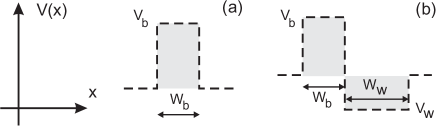
Figure 1: (a) A 1D potential barrier of height $V_{b}$ and width $W_{b}$. (b) A single unit of a potential well next to a potential barrier.

The model barriers and wells we consider are shown in Fig. 1(a). It is interesting to look at the tunneling through such barriers, which was previously studied by (Katsnelson et al., 2006) for a single barrier. This was later extended to massive electrons with spatially varying mass (Gomes & Peres, 2008).

Transmission. To find the transmission $T$ through a square-barrier structure one first observes that the wave function in the $j$th region $\psi_{j}(x)$ of the constant potential $V_{j}$ is given by a superposition of the eigenstates given by Eq. (2),

$$\psi_{j}(x)=A_{j}{\psi_{r}}_{j}+B_{j}{\psi_{l}}_{j}.$$ (4)

The wave function should be continuous at the interfaces. This boundary condition gives the transfer matrix $\mathcal{N}_{j}$ relating the coefficients $A_{j}$ and $B_{j}$ of region $j$ with those of the region $j+1$ in the manner

$$\begin{pmatrix}A_{j}\\ B_{j}\end{pmatrix}=\mathcal{N}_{j+1}\begin{pmatrix}A_{j+1}\\ B_{j+1}\end{pmatrix}.$$ (5)

By employing the transfer matrix at each potential step we obtain, after $n$ steps, the relation

$$\begin{pmatrix}A_{0}\\ B_{0}\end{pmatrix}=\prod^{n}_{j=1}\mathcal{N}_{j}\begin{pmatrix}A_{n}\\ B_{n}\end{pmatrix}.$$ (6)

In the region to the left of the barrier we assume $A_{0}=1$ and denote by $B_{0}=r$ the reflection amplitude. Likewise, to the right of the $n$th barrier we have $B_{n}=0$ and denote by $A_{n}=t$ the transmission amplitude.

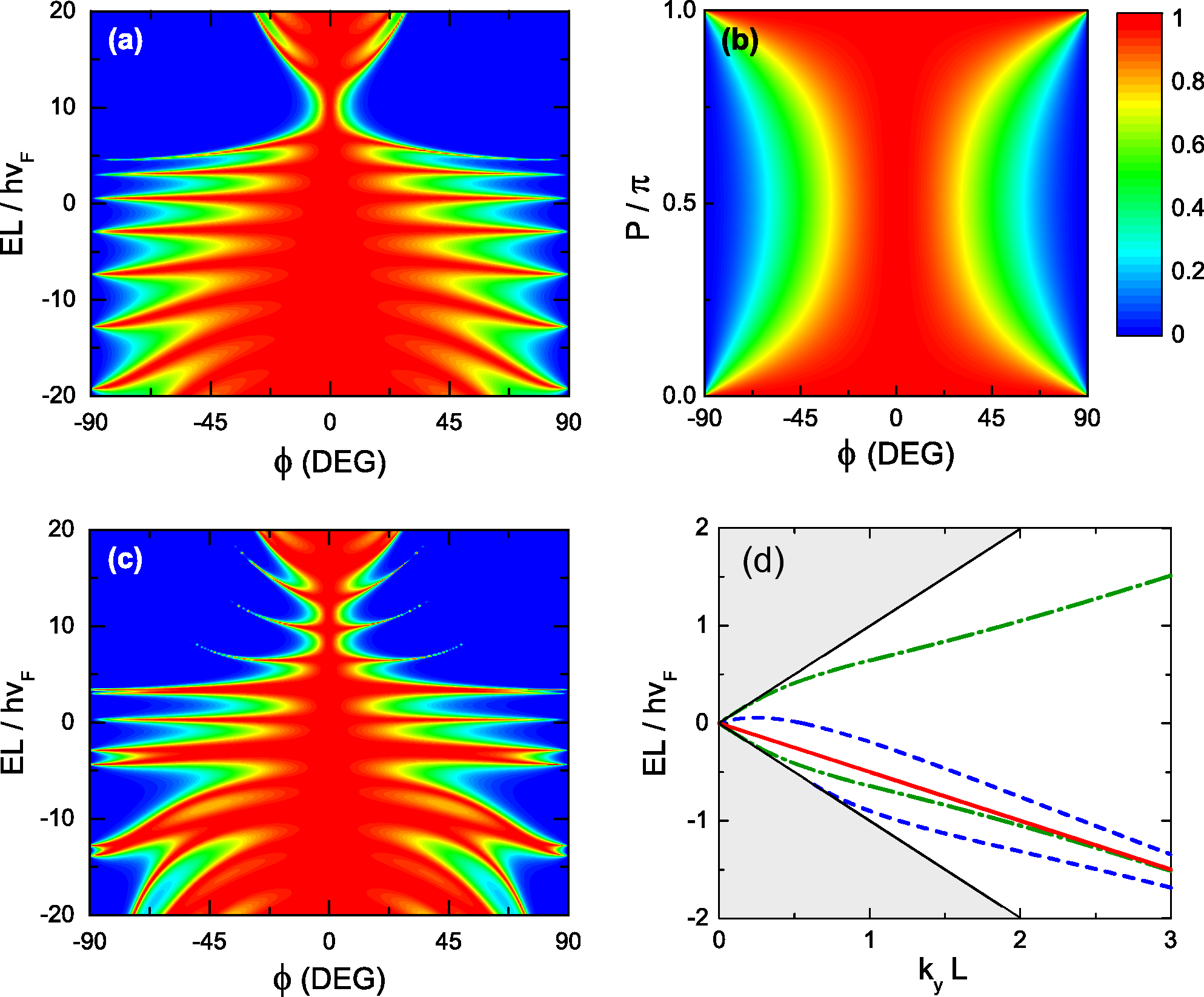
Figure 2: (a) Contour plot of the transmission through a single barrier with $\mu=0$, $W_{b}=L$, and $u_{b}=10$. (b) As in (a) for a single $\delta$-function barrier with $\mu=0$ and $u(x)=P\delta(x)$; the transmission is independent of the energy. (c) As in (a) for two barriers with $\mu=0$, $u_{b}=10$, $u_{w}=0$, $W_{b}=0.5L$, and $W_{w}=L$. (d) Spectrum of the bound states vs $k_{y}$ for a single ($L=1$, solid red line), two parallel (dashed blue curves), and two anti-parallel (green dash-dotted curves) $\delta$-function barriers ($L$ is the inter-barrier distance).

The transmission probability $T$ can be expressed as the ratio of the transmitted current density $j_{x}$ over the incident one, where $j_{x}=v_{F}\psi^{\dagger}\sigma_{x}\psi$. This results in $T=(\lambda^{\prime}/\lambda)|t|^{2}$, with $\lambda^{\prime}/\lambda$ the ratio between the wave vector $\lambda^{\prime}$ to the right and $\lambda$ to the left of the barrier. If the potential to the right and left of the barrier is the same we have $\lambda^{\prime}=\lambda$. For a single barrier the transmission amplitude is given by $T=|t|^{2}=|N_{11}|^{-1}$, with $N_{ij}$ the elements of the transfer matrix $\mathcal{N}$. Explicitly, $t$ can be written as

$$1/t=\cos(\lambda_{b}W_{b})-iQ\sin(\lambda_{b}W_{b}),$$ (7)

$$Q=(\varepsilon_{0}\varepsilon_{b}-k_{y}^{2}-\mu_{0}\mu_{b})/\lambda_{0}\lambda_{b};$$

the indices $0$ and $b$ refer, respectively, to the region outside and inside the barrier and $\varepsilon_{b}=\varepsilon-u$. A contour plot of the transmission is shown in Fig. 2(a). We clearly see: 1) $T=1$ for $\phi=0$ which is the well-known Klein tunneling, and 2) strong resonances, in particular for $E<0$, when $\lambda_{b}W_{b}=n\pi$, which describe hole scattering above a potential well.

In the limit of a very thin and high barrier, one can model it by a $\delta$-function barrier $V(x)/\hbar v_{F}=P\delta(x)$. Using Eq. (7) for $t$ gives (Barbier et al., 2009a)

$$T=1/[1+\sin^{2}P\tan^{2}\phi],$$ (8)

with $\tan\phi=k_{y}/\lambda_{0}$ the angle of incidence. Notice that this transmission is independent of the energy and is a periodic function of $P$. The latter is very different from the non-relativistic case where T is a decreasing function of P. A contour plot of the transmission is shown in Fig. 2(b) and $T=1$ for $\phi\approx 0$ which is nothing else than Klein tunneling. Notice also the symmetry $T(\pi-P)=T(P)$.

For two barriers the system becomes a resonant structure, for which it was found that the resonances in the transmission depend mostly on the width $W_{w}$ of the well between the barriers (Pereira Jr et al., 2007a). A plot of the transmission is shown in Fig. 2(c). In the limit of two parallel $\delta$-function barriers of equal strength $P$ we obtain the transmission

$$T=\big{[}1+\tan^{2}\phi(\cos\lambda_{0}\sin 2P-2s\sin\lambda_{0}\sin^{2}P/\cos\phi)^{2}\big{]}^{-1}.$$ (9)

The case of two anti-parallel $\delta$-function barriers of equal strength is also interesting. The relevant transmission is

$$T=\big{[}\cos^{2}\lambda_{0}+\sin^{2}\lambda_{0}(1-\sin^{2}\phi\cos 2P)^{2}/\cos^{4}\phi\big{]}^{-1}.$$ (10)

Conductance. The two-terminal conductance is given by

$$G(E_{F})=G_{0}\int_{-\pi/2}^{\pi/2}T(E_{F},\phi)\cos\phi\,\rd\phi,$$ (11)

with $G_{0}=2E_{F}L_{y}e^{2}/(v_{F}h^{2})$ for single-layer graphene, and $L_{y}$ the width of the system. For a single and double barrier, the transmission through which is plotted in Fig. 2(a) and 2(c), the conductance $G$ is shown in Fig. 3(b) and exhibits multiple resonances despite the integration over the angle $\phi$.

Taking the limit of a $\delta$-function barrier leads to $G$ periodic in $P$ and given by

$$G/G_{0}=2\big{[}1-\text{artanh}(\cos P)\sin P\tan P\big{]}/\cos^{2}P.$$ (12)

For one period $G$ is shown in Fig. 3(a).

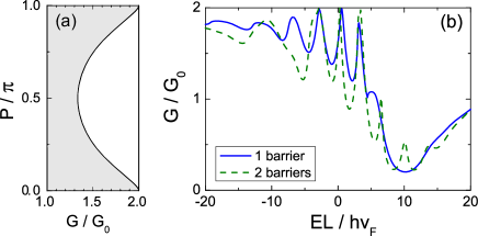
Figure 3: (a) Conductance $G$ vs strength $P$ of a $\delta$-function barrier in single-layer graphene; the conductance is independent of the energy. (b) Conductance $G$ vs energy for the single (solid blue curve) and double (dashed green curve) square barrier of Fig. 2(a) and 2(c).

Bound states. For $k_{y}^{2}+\mu_{0}^{2}>\varepsilon^{2}$ the wave function outside the barrier (well) becomes an exponentially decaying function of $x$, $\psi(x)\propto\exp\{\pm|k_{x}|x\}$ with $|k_{x}|=[k_{y}^{2}+\mu_{0}^{2}-\varepsilon^{2}]^{1/2}$. Localized states form near the barrier boundaries (Pereira Jr et al., 2006); however, they are propagating freely along the $y$-direction. The spectrum of these bound states can be found by setting the determinant of the transfer matrix equal to zero. For a single potential barrier (well) it is given by the solution of the transcendental equation

$$|\lambda_{0}|\lambda_{b}\cos(\lambda_{b}W_{b})+(k_{y}^{2}+\mu_{0}\mu_{b}-\varepsilon(\varepsilon-u))\sin(\lambda_{b}W_{b})=0.$$ (13)

In Fig. 4(b) these bound states are shown, as a function of $k_{y}$, by the dashed blue (red) curves.

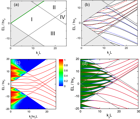
Figure 4: (a) Four different regions for a single unit of Fig. 1(b) with $u_{b}=24$, $u_{w}=16$, $W_{b}=0.4$ and $W_{w}=0.6$. The green line corresponds to region I in the limit of a $\delta$-function barrier. (b) Bound states for a single barrier (dashed blue curves) and well (dashed red curves) and the combined barrier-well unit (black curves). (c) Contour plot of the transmission through a unit with $\mu=2$, $u_{b}=-u_{w}=20$ and $W_{b}=W_{w}=0.5$; the red curves show the bound states. (d) Spectrum of a SL whose unit cell is shown in Fig. 1(b), for $k_{x}=0$ (blue curves) and $k_{x}L=\pi/2$ (red curves).

An interesting structure to study is that of a potential barrier next to a well but with average potential equal to zero, considered by (Arovas et al., 2010). This is the unit cell (shown in Fig. 1(b)) of the SL we will use in Sec. 3 where extra Dirac points will be found. In Fig. 4(a) the Dirac cone outside the barrier is shown as a grey area, inside this region there are no bound states. Superimposed are grey lines corresponding to the edges of the Dirac cones inside the well and barrier that divide the $(E,k_{y})$ plane into four regions. Region I corresponds to propagating states inside both the barrier and well while region II (III) corresponds to propagating states only inside the well (barrier). In region IV no propagating modes are possible, neither in the barrier nor in the well. For high thin barriers, region I will become a thin area adjacent to the upper cone, converging to the dark green line in the limit of a $\delta$-function barrier. Figure 4(b) shows that the bound states of this structure are composed of the ones of a single barrier and those of a single well. Anticrossings take place where the bands otherwise would cross. The resulting spectrum is clearly a starter of the spectrum of a SL shown in Fig. 4(d).

In the limit of $\delta$-function barriers and wells the expressions for the dispersion relation are strongly simplified by setting $\mu=0$ in all regions. For a single $\delta$-function barrier the bound state is given by

$$\varepsilon=\sgn(\sin P)|k_{y}|\cos P,$$ (14)

which is a straight line with a reduced group velocity $v_{y}$; the result is shown in Fig. 2(d) by the red curve. Comparing with the single-barrier case we notice that due to the periodicity in $P$, the $\delta$-function barrier can act as a barrier or as a well depending on the value of $P$.

For two $\delta$-function barriers there are two important cases: the parallel and the anti-parallel case. For parallel barriers one finds an implicit equation for the energy

$$|\lambda^{\prime}\cos P+\varepsilon\sin P|=|\re^{-\lambda^{\prime}}k_{y}\sin P|,$$ (15)

where $\lambda^{\prime}=|\lambda_{0}|$, while for anti-parallel barriers one obtains

$$k_{y}^{2}\sin^{2}P=\lambda^{\prime 2}/(1-\re^{-2\lambda^{\prime}}).$$ (16)

For two (anti-)parallel $\delta$-function barriers we have, for each fixed $k_{y}$ and $P$, two energy values $\pm\varepsilon$, and therefore two bound states. In both cases, for $P=n\pi$ the spectrum is simplified to the one in the absence of any potential $\varepsilon=\pm|k_{y}|$. In Fig. 2(d) the bound states for double (anti-)parallel $\delta$-function barriers are shown, as a function of $k_{y}L$, by the dashed blue (dash-dotted green) curves. For anti-parallel barriers we see that there is a symmetry around $E=0$, which is absent when the barriers are parallel.

2.2 Superlattice

Now we will consider the system of a superlattice with a corresponding 1D periodic potential, with square barriers, given by

$$V(x)=V_{0}\sum_{j=-\infty}^{\infty}[\Theta(x-jL)-\Theta(x-jL-W_{b})].$$ (17)

with $\Theta(x)$ the step function. The corresponding wave function is a Bloch function and satisfies the periodicity condition $\psi(L)=\psi(0)\exp(ik_{x})$, with $k_{x}$ now the Bloch phase. Using this relation together with the transfer matrix for a single unit $\psi(L)=\mathcal{M}\psi(0)$ leads to the condition

$$\det[\mathcal{M}-\exp(ik_{x})]=0.$$ (18)

This gives the transcendental equation

$$\cos k_{x}=\cos\lambda_{w}W_{w}\cos\lambda_{b}W_{b}-Q\sin\lambda_{w}W_{w}\sin\lambda_{b}W_{b},$$ (19)

from which we obtain the energy spectrum of the system. In Eq. (19) we used the following notation:

$$\varepsilon_{w}=\varepsilon+uW_{b},\quad\varepsilon_{b}=\varepsilon-uW_{w},\quad u=V_{0}L/\hbar v_{F},\quad W_{b,w}\rightarrow W_{b,w}/L,$$

$$\lambda_{w}=[\varepsilon_{w}^{2}-k_{y}^{2}-\mu_{w}^{2}]^{1/2},\quad\lambda_{b}=[\varepsilon_{b}^{2}-k_{y}^{2}-\mu_{b}^{2}]^{1/2},\quad Q=(\varepsilon_{w}\varepsilon_{b}-k_{y}^{2}-\mu_{b}\mu_{w})/\lambda_{w}\lambda_{b}.$$

Numerical results for the dispersion relation $E(k_{y})$ are shown in Fig. 4(d). We see the appearance of bands (green areas) which for large $k_{y}$ values collapse into the bound states (where the red and blue curves meet) while the charge carriers move freely along the $y$ direction.

2.3 Collimation and extra Dirac points

As shown by various studies, carriers in graphene SLs exhibit several interesting pecularities that result from the particular electronic SL band structure. In a 1D SL it was found that the spectrum can be altered anisotropically (Park et al., 2008a; Bliokh et al., 2009). Moreover, this anisotropy can be made very large such that for a broad region in k space the spectrum is dispersionless in one direction, and thus electrons are collimated along the other direction (Park et al., 2009a). Even more intriguing was the ability to split off ”extra Dirac points” (Ho et al., 2009) with accompanying zero modes (Brey & Fertig, 2009) which move away from the K point along the $k_{y}$ direction with increasing potential strength. Here we will describe these phenomena for a SL of square potential barriers.

We start by describing the collimation as done by (Park et al., 2009a); subsequently we will find the conditions on the parameters of the SL for which a collimation appears. It turns out that they are the same as those needed to create a pair of extra Dirac points.

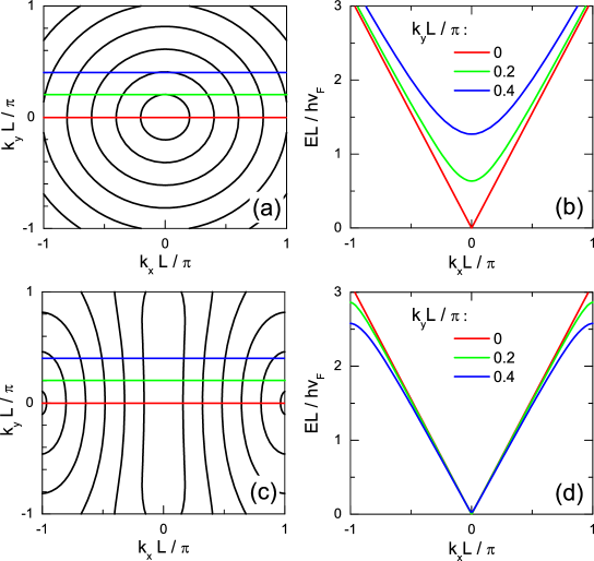
Figure 5: The lowest conduction band of the spectrum of graphene near the K point in the absence of SL potential (a), (b) and in its presence (c), (d) with $u=4\pi$. (a) and (c) are contour plots of the conduction band with a contour step of $0.5$ $\hbar v_{F}/L$. (b) and (d) show slices along constant $k_{y}L=0,0.2,0.4\pi$.

Following (Park et al., 2009a) the condition for collimation to occur is $\int_{BZ}\re^{\ri s\hat{s}\alpha(x)}=0$, where the function $\alpha(x)=2\int^{x}_{0}u(x^{\prime})\rd{x^{\prime}}$ embodies the influence of the potential, $s=\text{sign}(\varepsilon)$ and $\hat{s}=\text{sign}(k_{x})$. For a symmetric rectangular lattice this corresponds to $u/4=n\pi$. The spectrum for the lowest energy bands is then given by (Park et al., 2008b)

$$\varepsilon\approx\pm\big{[}k_{x}^{2}+|f_{l}|^{2}k_{y}^{2}\big{]}^{1/2}+\pi l/L$$ (20)

with $f_{l}$ being the coefficients of the Fourier expansion $\re^{\ri\alpha(x)}=\sum_{l=-\infty}^{\infty}f_{l}\re^{\ri 2\pi lx/L}$. The coefficients $f_{l}$ depend on the potential profile $V(x)$, with $|f_{l}|<1$. For a symmetric SL of square barriers we have $f_{l}=u\sin(l\pi/2-u/2)/(l^{2}u^{2}-u^{2}/4)$. The inequality $|f_{l}|<1$ implies a group velocity in the $y$ direction $v_{y}<v_{F}$ which can be seen from Eq. (20).

In Fig. 5(b),(d) we show the dispersion relation $E$ vs $k_{x}$ for $u=4\pi$ at constant $k_{y}$. As can be seen, when a SL is present in most of the Brillouin zone the spectrum, partially shown in (c), is nearly independent of $k_{y}$. That is, we have collimation of an electron beam along the SL axis. The condition $u=V_{0}L/\hbar v_{F}=4n\pi$ shows that altering the period of the SL or the potential height of the barriers is sufficient to produce collimation. This makes a SL a versatile tool for tuning the spectrum. Comparing with Figs. 5(a), (b) we see that the cone-shaped spectrum for $u=0$, is transformed into a wedge-shaped spectrum (Park et al., 2009a).

We will compare this result now with an other approximate result for the spectrum, where we suppose $\varepsilon$ small instead of $k_{y}$ small. We start with the transcendental equation (19). As we are interested in an analytical approximate expression for the spectrum, we choose to expand the dispersion relation around $\varepsilon=0$ up to second order in $\varepsilon$. The resulting spectrum is

$$\varepsilon_{\pm}=\pm\left[{\frac{4|a^{2}|^{2}\,\big{[}k_{y}^{2}\sin^{2}(a/2)+a^{2}\sin^{2}(k_{x}/2)\big{]}}{k_{y}^{4}a\sin a+a^{2}u^{4}/16-2k_{y}^{2}u^{2}\sin^{2}(a/2)}}\right]^{1/2},$$ (21)

with $a=[u^{2}/4-k_{y}^{2}]^{1/2}$. In order to compare this spectrum with that by (Park et al., 2009a), we expand Eq. (19) for small ${\bf k}$ and $\varepsilon$; this leads to

$$\varepsilon\approx\pm\big{[}k_{x}^{2}+k_{y}^{2}\,\sin^{2}(u/4)/(u/4)^{2}\big{]}^{1/2}.$$ (22)

This spectrum has the form of an anisotropic cone and corresponds to that of Eq. (20) for $l=0$ (higher $l$ correspond to higher energy bands). In Fig. 6(a), (b) we see that the cone-shaped spectrum in (a), for $u=0$, is transformed into a anisotropic spectrum in (b), for $u=4.5\pi$, having peculiar extra Dirac points. These extra Dirac points cannot be described by a spectrum having an anisotropic cone-shape, therefore we compare the two approximate spectra. In Fig. 6(c), (d) we show how Eq. (21)) and Eq. (22) differ from the “exact” numerically obtained spectrum. From this figure one can see that Eq. (21) describes the lowest bands rather well for $\varepsilon<1$, while Eq. (22) is sufficient to describe the spectrum near the Dirac point. The former equation will be usefull when describing the spectrum near the extra Dirac points and we will use it to obtain the velocity.

We now move on to another important feature of the spectrum, the extra Dirac points first obtained by (Ho et al., 2009) using tight-binding calculations. These extra Dirac points are found as the zero-energy solutions of the dispersion relation in Eq. (19) for zero energy (Barbier et al., 2010).

In order to find the location of the Dirac points we assume $k_{x}=0$, $\varepsilon=0$, $\mu_{b}=\mu_{w}=0$, and consider the special case of $W_{b}=W_{w}=1/2$ in Eq. (19). The resulting equation

$$1=\cos^{2}\lambda/2+\big{[}(u^{2}/4+k_{y}^{2})/(u^{2}/4-k_{y}^{2})\big{]}\,\sin^{2}\lambda/2,$$ (23)

has solutions for $u^{2}/4-k_{y}^{2}=u^{2}/4+k_{y}^{2}$ or $\sin^{2}\lambda/2=0$. This determines the values of $k_{y}=0$ (at the Dirac points) as

$$k_{y,j\pm}=\pm\sqrt{\frac{u^{2}}{4}-4j^{2}\pi^{2}};$$ (24)

the extra Dirac points are for $j\neq 0$. For a SL spectrum symmetric around zero energy, the extra Dirac points are at $\varepsilon=0$. We expect from the considerations of Sec. 2(2.2) (and Fig. 4(b)) that for unequal barrier and well widths this will no longer be true. Indeed, in such a case the extra Dirac points shift in energy, as seen in Fig. 4(d), and their position in the spectrum is given, for $k_{x}=0$, by (Barbier et al., 2010)

$$\varepsilon_{j,m}=\frac{u}{2}(1-2W_{b})+\frac{\pi^{2}}{2u}\left(\frac{j^{2}}{W_{w}^{2}}-\frac{(j+2m)^{2}}{W_{b}^{2}}\right),$$ (25)

$${k_{y}}_{j,m}=\pm\Big{[}(\varepsilon_{j,m}+uW_{b})^{2}-(j\pi/W_{w})^{2}\Big{]}^{1/2},$$

where $j$ and $m$ are integers, and $m\neq 0$ corresponds to higher and lower crossing points. Also, perturbing the potential with an asymmetric term, as done by (Park et al., 2009b), leads to qualitatively similar results.

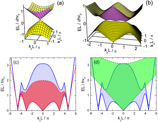
Figure 6: The spectrum of graphene near the K point in the absence of a SL (a) and in its presence (b) with $u=4.5\pi$. (c) and (d) The SL spectrum with $u=10\pi$, the lowest conduction bands are coloured in cyan, red, and green for, respectively, the exact, and the approximations given by (c) Eq. (21) and (d) Eq. (22), respectively. The approximate spectra are delimited by the dashed curves.

An investigation of the group velocity near the (extra) Dirac points is appropriate for understanding the transport of carriers in the energy bands close to zero energy. Near the extra Dirac points the group velocity tends to renormalise differently as compared to the original Dirac point. Near them ${\bf v}$ is oriented along the $y$ direction, while near the latter one ${\bf v}$ is oriented along the $x$ direction (Ho et al., 2009). The group velocity near the extra Dirac points can be calculated from Eq. (21). At the $j$th extra Dirac point the magnitude of the velocity ${\bf v}/v_{F}=(\partial\varepsilon/\partial k_{x},\,\partial\varepsilon/\partial k_{y})$ is given by

$$v_{x}/v_{F} =16\pi^{2}j^{2}\cos(k_{x}/2)/u^{2}$$ (26)

$$v_{y}/v_{F} =(u^{2}/4-4j^{2}\pi^{2})/u^{2},$$

while at the main Dirac point it is given by $v_{x}/v_{F}=1$ and $v_{y}/v_{F}=4\sin(u/4)/u$. The dependence of the velocity components on the strength of the potential barriers is shown in Fig. 7. From this figure we observe that new extra Dirac points emerge upon increasing $u=V_{0}L/\hbar v_{F}$ (consistent with Eq. (24)) and $v_{x}$ decreases while $v_{y}$ increases. The Dirac point itself, however, shows a different behaviour upon increasing $u$, namely $v_{x}=v_{F}$ constant, and $v_{y}$ is here a globally decaying function showing $v_{y}=0$ for periodic values of $u$, $u=4n\pi$, with $n$ a nonzero positive integer.

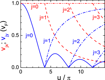
Figure 7: The group velocity components $v_{y}$ and $v_{x}$ at the Dirac point $j=0$ (shown, respectively, by the solid blue and the dot-dot-dashed red curve), and at the extra Dirac points $j=1,2,3$ (shown, respectively, by the dot-dashed blue and the dashed red curves) as a function of the barrier parameter $u=V_{0}L/\hbar v_{F}$.

Conductivity. We now turn to the transport properties of a SL and look at the influence of these extra Dirac points on the conductivity. The diffusive dc conductivity $\sigma_{\mu\nu}$ for the SL system can be readily calculated from the spectrum if we assume a nearly constant relaxation time $\tau(E_{F})\equiv\tau_{F}$. It is given by (Charbonneau et al., 1982)

$$\sigma_{\mu\nu}(E_{F})=\frac{e^{2}\beta\tau_{F}}{A}\sum_{n,\bf{k}}v_{n\mu}v_{n\nu}f_{n\bf{k}}(1-f_{n\bf{k}}),$$ (27)

with $A$ the area of the system, $n$ the energy band index, $\mu,\,\nu=x,y,$ and $f_{n\bf{k}}=1/[\exp(\beta(E_{F}-E_{n\bf{k}}))+1]$ the equilibrium Fermi-Dirac distribution function; $\beta=1/k_{B}T$ and the temperature enters the results through the dimensionless value for $\beta$ which is $\beta=\hbar v_{F}/k_{B}TL=20$.

For comparison we first look at the conductivity tensor at zero temperature and in the absence of a SL. For single-layer graphene the conductivity is given by

$$\sigma_{\mu\mu}(\varepsilon_{F})/\sigma_{0}=\varepsilon_{F}/4\pi$$ (28)

with $\sigma_{0}=e^{2}/\hbar$,

In Figs. 8(a), (b) the conductivities $\sigma_{xx}$ and $\sigma_{yy}$ are shown for a SL as functions of the energy. Notice that for small energies the slope of the conductivity $\sigma_{yy}$ is tunable to a large extent by altering the parameter $u$ of the SL. The dashed blue curves correspond to $u=4\pi$ and the rather flat dispersion in the $y$ direction for the lowest conduction band (see Fig. 5(c,d)) translates to a small $\sigma_{yy}$ (for energies $EL/\hbar v_{F}<1$) compared to the conductivity in the absence of a SL. The solid red curves on the other hand correspond to $u=6\pi$ and due to the extra Dirac points, which have a rather flat dispersion in the $x$ direction (Ho et al., 2009), the conductivity $\sigma_{yy}$ is large.

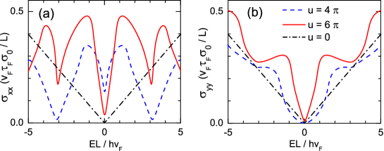
Figure 8: (Color online) Conductivities, $\sigma_{xx}$ in (a) and $\sigma_{yy}$ in (b), vs Fermi energy for a SL on single-layer graphene with $u=4\pi$ and $6\pi$ for, respectively, the blue dashed and red solid curves. In both cases $W_{b}=W_{w}=0.5$. The dash-dotted black curves show the conductivities in the absence of the SL potential, $\sigma_{xx}=\sigma_{yy}=\varepsilon_{F}\sigma_{0}/4\pi$.

2.4 Dirac lines

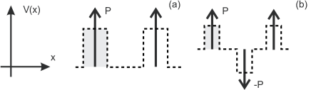
Figure 9: (a) Schematics of Kronig-Penney SL on single-layer graphene. (b) Extended Kronig-Penney SL.

In an effort to simplify the expressions for the dispersion relation we replace, as we did for the few-barrier structures, the SL barriers by $\delta$-function barriers. The square SL potential is then approximated by

$$V(x)=P\sum_{j=-\infty}^{\infty}\delta(x-jL).$$ (29)

This potential leads to the dispersion relation

$$\cos k_{x}=\cos\lambda\cos P+(\varepsilon/\lambda)\sin\lambda\sin P,$$ (30)

which is periodic in $P$. This is in sharp contrast with that for standard electrons which is not periodic in $P$ and which in our notation reads

$$\cos k_{x}=\cos\lambda^{\prime}+(\mu P/\lambda^{\prime})\sin\lambda^{\prime},$$ (31)

where $\mu=mv_{F}L/\hbar$ and $\lambda^{\prime}=[2\mu\varepsilon-k_{y}^{2}]^{1/2}$. As can be seen from Fig. 10(a), the energy band near the Dirac point has the interesting property that it becomes nearly flat in $k_{x}$, forming a plane, for large $k_{y}$. The angle which the asymptotic plane makes with the zero-energy plane depends on $P$ and the group velocity $v_{y}$ corresponding to this asymptotic plane varies from $-v_{F}$ to $v_{F}$ in each period $n\pi<P<(n+1)\pi$. Notice that no extra Dirac points are found and the reason is the same as that for the asymmetric SL potential, i.e., the extra Dirac points shift away from zero energy. Alternatively, we can try to shed some light by comparing with Sec. 2(2.2), where it is explained that the bound states for a single unit of the SL potential are similar to those of the combined single barrier and well. In the region where the bound states cross (denoted by I in Fig. 4(a)) anti-crossings occur and corresponding crossings in the SL spectrum (extra Dirac points) are expected. In the limit of a $\delta$-function barrier this region is reduced to a line (the dark green line in Fig. 4(a)). This prevents anti-crossings from occurring and in this way no extra Dirac points are expected.

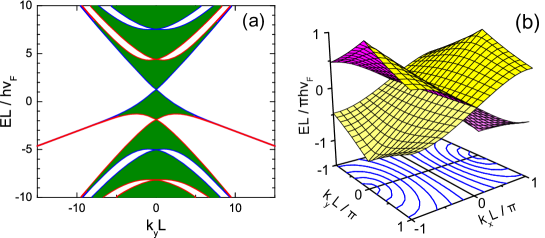
Figure 10: (a) Spectrum for a Kronig-Penney SL with $P=0.4\pi$. The blue and red curves show, respectively, the $k_{x}=0$ and $k_{x}=\pi/L$ results which delimit the energy bands (green coloured regions). (b) Spectrum for an extended Kronig-Penney SL with $P=\pi/2$. Notice that the Dirac point has become a Dirac line.

Extended Kronig-Penney model. To re-establish the symmetry between electrons and holes, as in the case of square barriers with $W_{b}=W_{w}$, we can use alternating-in-sign $\delta$-function barriers. The unit cell of the periodic potential contains one such barrier up, at $x=0$, followed by a barrier down, at $x=L/2$, see Fig. 9(b). The potential is given by

$$V(x)=P\sum_{j=-\infty}^{\infty}[\delta(x-jL)-\delta(x-jL-L/2)],$$ (32)

and is the asymptotic limit of the potential shown in Fig. 1(b). The resulting transfer matrix leads to the dispersion relation

$$\cos k_{x}=\cos\lambda-(2k_{y}^{2}/\lambda^{2})\sin^{2}(\lambda/2)\sin^{2}P.$$ (33)

This dispersion relation is periodic in $P$. As shown in Fig. 10(b) no extra Dirac points occur, but for the particular case of $P=(n+1/2)\pi$, $n$ an integer, the spectrum shows an interesting feature: for all $k_{y}$ we see that Eq. (33) has a solution with $\varepsilon=k_{x}=0$, which means the Dirac point at $k_{x}=k_{y}=0$ turned into a Dirac line along the $k_{y}$ axis. If we take $k_{y}$ not too large (of the order of $k_{x}$), this spectrum has a wedge structure as was also found for rectangular SLs. For $k_{y}\rightarrow\infty$, though, the spectrum becomes a horizontal plane situated at $\varepsilon=0$. We can generalize this model by taking the distance $W$ between the two barriers of the unit cell not equal to $L/2$. This was done by (Ramizani Masir et al., 2010, unpublished work). They found an approximate analytic expression for the dispersion given by

$$\varepsilon\approx[k_{x}^{2}+Fk_{y}^{2}]^{1/2},\qquad F=W^{2}+(L-W)^{2}+2W(L-W)\cos(2P).$$ (34)

This dispersion has the shape of an anisotropic cone with a renormalized velocity in the $y$ direction. Comparing with Eqs. (20) and (22), we observe that the condition for collimation and the velocity renormalization in the $y$ direction is quite different for square barriers. For instance, in the extended KP model, with $W=L/2$, we find $v_{y}/v_{F}=|\cos P|$ while for square barriers the result is $v_{y}/v_{F}=\sin(u/4)/(u/4)$. The latter means that if we consider $P\equiv u/4$, the velocity in the $y$ direction is maximum $v_{y}=v_{F}$ for $P=(1/2+n)\pi$ in the extended KP model while for square barriers $v_{y}=0$ at these points.

3 Bilayer graphene

We now turn to bilayer graphene and use again the nearest-neighbour, tight-binding Hamiltonian in the continuum approximation with ${\bf k}$ close to the $K$ point. If we include a potential difference between the two layers, the Hamiltonian is given by

$$\mathcal{H}=\begin{pmatrix}U_{1}&v_{F}\pi&t_{\perp}&0\\ v_{F}\pi^{\dagger}&U_{1}&0&0\\ t_{\perp}&0&U_{2}&v_{F}\pi^{\dagger}\\ 0&0&v_{F}\pi&U_{2}\end{pmatrix}.$$ (35)

Here $U_{1}$ and $U_{2}$ are the potentials on layers $1$ and $2$, respectively, $2\Delta=U_{1}-U_{2}$ is the potential difference, and $t_{\perp}$ describes the coupling between the layers. The energy spectrum for free electrons is given by (McCann, 2006; Barbier et al., 2009b)

$$\varepsilon =u_{0}\pm\Big{[}\Delta^{2}+k^{2}+\frac{t^{2}_{\perp}}{2}+(4\Delta^{2}k^{2}+k^{2}t^{2}_{\perp}+\frac{t^{2}_{\perp}}{4})^{1/2}\Big{]}^{1/2},$$ (36)

$$\varepsilon =u_{0}\pm\Big{[}\Delta^{2}+k^{2}+\frac{t^{2}_{\perp}}{2}-(4\Delta^{2}k^{2}+k^{2}t^{2}_{\perp}+\frac{t^{2}_{\perp}}{4})^{1/2}\Big{]}^{1/2},$$

with $u_{1}=u_{0}+\Delta$ and $u_{2}=u_{0}-\Delta$. Contrary to Sec. 3 we use units in inverse distance, namely, $\varepsilon=E/\hbar v_{F}$, $u_{j}=U_{j}/\hbar v_{F}$, and $k=[\lambda^{2}+k_{y}^{2}]^{1/2}$. This spectrum exhibits an energy gap that for $2\Delta\ll t_{\perp}$ equals the difference $2\Delta$ between the conduction and valence band at the K point (McCann, 2006).

Solutions for this Hamiltonian are four-vectors $\psi$ and for 1D potentials we can write $\psi(x,y)=\psi(x)\exp(ik_{y}y)$. If the potentials $U_{1}$ and $U_{2}$ do not vary in space, these solutions are of the form

$$\Psi_{\pm}(x)=\begin{pmatrix}1\\ f_{\pm}\\ h_{\pm}\\ g_{\pm}h_{\pm}\end{pmatrix}e^{\pm\ri\lambda x+\ri k_{y}y},$$ (37)

with $f_{\pm}=[-\ri k_{y}\pm\lambda]/[\varepsilon^{\prime}-\delta]$, $h_{\pm}=[(\varepsilon^{\prime}-\delta)^{2}-k_{y}^{2}-\lambda^{2}]/[t_{\perp}(\varepsilon^{\prime}-\delta)]$, and $g_{\pm}=[ik_{y}\pm\lambda]/[\varepsilon^{\prime}+\delta]$; the wave vector $\lambda$ is given by

$$\lambda_{\pm}=\left[\varepsilon^{\prime 2}+\delta^{2}-{k_{y}}^{2}\pm\sqrt{4\varepsilon^{\prime 2}\delta^{2}+t_{\perp}^{2}(\varepsilon^{\prime 2}-\delta^{2})}\right]^{1/2}.$$ (38)

We will write $\lambda_{+}=\alpha$ and $\lambda_{-}=\beta$.

3.1 Tuning of the band offsets

It was shown before that using a 1D biasing, indicated in Figs. 11(a,b,c) by $2\Delta$, one can create three types of heterostructures in graphene (Dragoman et al., 2010). A fourth type, where the energy gap is spatially kept constant but the bias periodically changes sign along the interfaces, can be introduced (see Fig. 11(d)). We characterize these heterostructures as follows:
1) Type I: The gate bias applied in the barrier regions is larger than in the well regions.
2) Type II: The gaps, not necessarily equal, are shifted in energy but they have an overlap as shown.
3) Type III: The gaps, not necessarily equal, are shifted in energy and have no overlap.
4) Type IV: The bias changes sign between successive barriers and wells but its magnitude remains constant.

Type IV structures have been shown to localize the wave function at the interfaces (Martin et al., 2008; Martinez et al., 2009). To understand the influence of such interfaces in this section we will separately investigate structures with such a single interface embedded by an anti-symmetric potential.

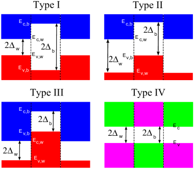
Figure 11: Four different types of band alignments in bilayer graphene. $E_{c,b},E_{c,w},E_{v,c}$, and $E_{v,b}$ denote the energies of the conduction (c) and valence (v) bands in the barrier (b) and well (w) regions. The corresponding gap is, respectively, $2\Delta_{b}$ and $2\Delta_{w}$.

To describe the transmission and bound states of some simple structures we notice that in the energy region of interest, i.e., for $|E|<t_{\perp}$, the eigenstates which are propagating are the ones with $\lambda=\alpha$. Accordingly, from now on we will assume that $\beta$ is complex. In this way we can simply use the transfer-matrix approach of Sec. 2 in the transmission calculations. This leads to the relation

$$\begin{pmatrix}t\\ 0\\ e_{d}\\ 0\end{pmatrix}=\mathcal{N}\begin{pmatrix}1\\ r\\ 0\\ e_{g}\end{pmatrix}.$$ (39)

Again the transmission is given by $T=|t|^{2}$.

For a single barrier the transmission in bilayer graphene is given by a complicated expression. Therefore, we will first look at a few limiting cases. First we assume a zero bias $\Delta=0$ that corresponds to a particular case of type III heterostructures. In this case we slightly change the definition of the wave vectors: for $\Delta=0$ we assume $\alpha(\beta)=[\varepsilon^{2}+(-)\varepsilon t_{\perp}-k_{y}^{2}]^{1/2}$. If we restrict the motion along the $x$ axis, by taking $k_{y}=0$, and assume a bias $\Delta=0$, then the transmission $T=|t|^{2}$ is given via

$$1/t =e^{i\alpha_{0}D}[\cos(\alpha_{b}D)-iQ\sin(\alpha_{b}D)],$$ (40)

$$Q =\frac{1}{2}\left(\frac{\alpha_{b}\varepsilon_{0}}{\alpha_{0}\varepsilon_{b}}+\frac{\alpha_{0}\varepsilon_{b}}{\alpha_{b}\varepsilon_{0}}\right).$$

This expression depends only on the propagating wave vector $\alpha$ ($\beta$ for $E<0$) as propagating and localized states are decoupled in this approximation. This also means that one does not find any resonances in the transmission for energies in the barrier region, i.e., for  $0<\varepsilon<u$. Due to the coupling for nonzero $k_{y}$ with the localized states, resonances in the transmission will occur (see Fig. 12). We can easily generalize this expression to account for the double barrier case under the same assumptions. With an inter-barrier distance $W_{w}$ one obtains the transmission (Barbier et al., 2009b) $T_{d}=|t_{d}|^{2}$ from

$$t_{d}=\frac{e^{i2\alpha_{0}(W_{w}+2W_{b})}|t|^{2}e^{i2\phi_{t}}}{1-|r|^{2}e^{i2\phi_{r}}e^{i2\alpha_{0}W_{w}}},$$ (41)

with $r=|r|\re^{\ri\phi_{r}}$, and $t=|t|\re^{\ri\phi_{t}}$, corresponding to the single barrier transmission and reflection amplitudes. In this case we do have resonances due to the well states; they occur for $\re^{\ri 2\phi_{r}}\re^{\ri 2\alpha_{0}W_{w}}=1$. As $\phi_{r}$ is independent of $W_{w}$, one obtains more resonances by increasing $W_{w}$.

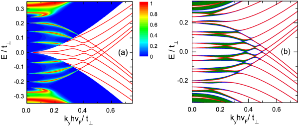
Figure 12: (a) Contour plot of the transmission for the potential of Fig. 1(b) in bilayer graphene with $W_{b}=W_{w}=40$ nm, $V_{b}=-V_{w}=100$ meV and zero bias. Bound states are shown by the red curves. (b) Spectrum for a SL whose unit is the potential structure of Fig. 1(b). Blue and red curves show, respectively, the $k_{x}=0$ and $k_{x}=\pi/L$ results which delimit the energy bands (green coloured regions).

For a single $\delta$-function barrier with potential $V(x)/\hbar v_{F}=P\delta(x)$ under zero bias, we find the transmission amplitude

$$1/t=\cos P+\ri\mu\sin P+\frac{(\alpha-\beta)^{2}k_{y}^{2}}{4\alpha\beta\varepsilon^{2}}\frac{\sin P}{\cot P+\ri\nu},$$ (42)

where $\mu=(\varepsilon+1/2)/\alpha$ and $\nu=(\varepsilon-1/2)/\beta$. Notice that this formula is periodic in the strength of the barrier $P$ as in the single-layer case.

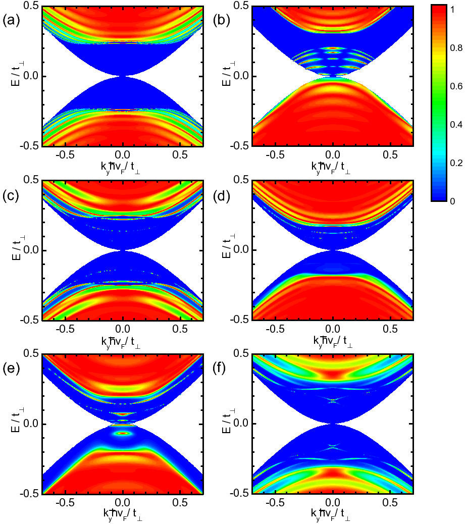
Figure 13: (Color online) Contour plot of the transmission through a single barrier in (a) and (b), for width $W_{b}=50$ nm, and through double barriers in (c), (d), (e), and (f) of equal widths $W_{b}=20$ nm that are separated by $W_{w}=20$ nm. Other parameters are as follows: (a) $\Delta_{b}=100$ meV, $V_{b}=0$ meV. (b) $\Delta_{b}=20$ meV, $V_{b}=50$ meV. (c) Type I: $V_{b}=V_{w}=0$ meV, $\Delta_{w}=20$ meV, and $\Delta_{b}=100$ meV. (d) Type II: $Vb=-Vw=20$ meV, $\Delta_{w}=\Delta=50$ meV, (e) Type III: $V_{b}=-V_{w}=50$ meV, $\Delta_{w}=\Delta_{b}=20$ meV. (f) Type IV: $V_{b}=V_{w}=0$ meV, $\Delta_{b}=-\Delta_{w}=100$ meV.

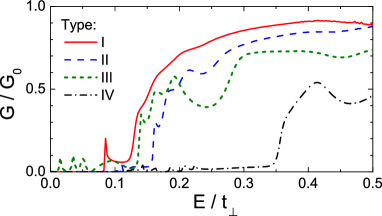
Figure 14: (Color online) Two-terminal conductance of four equally spaced barriers vs energy for $W_{b}=W_{w}=10$ nm and different SL types I-IV. The solid red curve (type I) is for $\Delta_{b}=50$ meV, $\Delta_{w}=20$ meV, and $V_{w}=V_{b}=0$. The blue dashed curve (type II) is for $\Delta_{b}=\Delta_{w}=50$ meV and $V_{b}=-V_{w}=20$ meV. The green dotted curve (type III) is for $\Delta_{b}=\Delta_{w}=20$ meV and $V_{b}=-V_{w}=50$ meV. The black dash-dotted curve (type IV) is for $\Delta_{b}=-\Delta_{w}=50$ meV and $V_{w}=V_{b}=0$.

For the general case we obtained numerical results for the transmission through various types of single and double barrier structures; they are shown in Fig. 13. The different types of structures clearly lead to different behaviour of the tunnelling resonances.

An interesting structure to study is the fourth type of SLs shown in Fig. 11(d). To investigate the influence of the localized states (Martin et al., 2008; Martinez et al., 2009) on the transport properties we embed the anti-symmetric potential profile in a structure with unbiased layers.

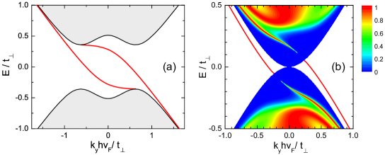
Figure 15: (a) Bound states of the anti-symmetric potential profile (type IV) with bias $\Delta_{w}=-\Delta_{b}=200$ meV. (b) Contour plot of the transmission through a $20$ nm wide barrier consisting of two regions with opposite biases $\Delta=\pm 100$ meV.

Conductance At zero temperature $G$ can be calculated from the transmission using Eq. (13) with $G_{0}=(4e^{2}L_{y}/2\pi h)\,(E_{F}^{2}+t_{\perp}E_{F})^{1/2}/\hbar v_{F}$ for bilayer graphene and $L_{y}$ the width of the sample. The angle of incidence $\phi$ is given by $\tan\phi=k_{y}/\alpha$ with $\alpha$ the wave vector outside the barrier. Figure 14 shows $G$ for the four SL types. Notice the clear differences in 1) the onset of the conductance and 2) the number and amplitude of the oscillations.

Bound states. To describe bound states we assume that there are no propagating states, i.e., $\alpha$ and $\beta$ are imaginary or complex (the latter case can be solved separately), and only the eigenstates with exponentially decaying behaviour are nonzero leading to the relation

$$\begin{pmatrix}f_{d}\\ 0\\ e_{d}\\ 0\end{pmatrix}=\mathcal{N}\begin{pmatrix}0\\ f_{g}\\ 0\\ e_{g}\end{pmatrix}.$$ (43)

From this relation we can find the dispersion relation for the bound states.

To study the localized states for the anti-symmetric potential profile (Martin et al., 2008; Martinez et al., 2009) we will use a sharp kink profile (step function). The spectrum found by the method above is shown in Fig. 15(a). We see that there are two bound states, both with negative group velocity $v_{y}\propto\partial{\varepsilon}/\partial{k_{y}}$, as found previously by (Martin et al., 2008). No bound state near zero energy was found for $k_{y}\rightarrow\infty$ in contradiction with (Martinez et al., 2009). For zero energy we find the solution

$$k_{y} =\pm\frac{1}{2}[\Delta^{2}+(\Delta^{4}+2\Delta^{2}t_{\perp}^{2})^{1/2}]^{1/2}$$ (44)

$$\approx\pm\sqrt{\Delta t_{\perp}}/2^{3/4},\quad\Delta\ll t_{\perp};$$

the approximation on the second line leads to the expression found by (Martin et al., 2008).

3.2 Superlattices

The heterostructures above (see Fig. 11), can be used to create four different types of SLs (Dragoman et al., 2010). We will especially focus on type IV and type III SLs in certain limiting cases.

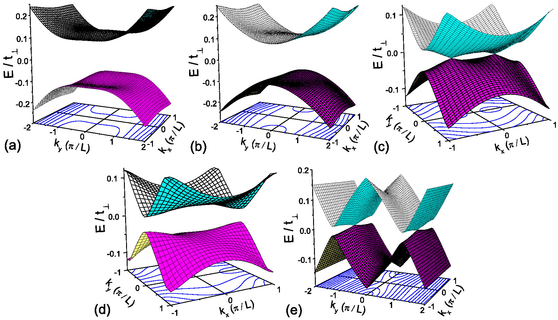
Figure 16: (Color online) Lowest conduction and highest valence band of the spectrum for a square SL with period $L=20$ nm and $W_{b}=W_{w}=10$ nm. (a) Type I: $\Delta_{b}=100$ meV and $\Delta_{w}=0$. (b) Type II: As in (a) for $\Delta_{b}=\Delta_{w}=50$ meV, and $V_{b}=-V_{w}=25$ meV. (c) Type III: $V_{b}=-V_{w}=25$ meV, and $\Delta_{b}=\Delta_{w}=0$. (d) Type III: $V_{b}=-V_{w}=50$ meV and $\Delta_{b}=\Delta_{w}=0$. (e) Type IV: Plot of the spectrum for a square SL with average potential $V_{b}=V_{w}=0$ and $\Delta_{b}=-\Delta_{w}=100$ meV. The contours are for the conduction band and show that the dispersion is almost flat in the $x$ direction.

For a type I SL we see in Fig. 16(a) that the conduction and valence band of the bilayer structure are qualitatively similar to those in the presence of a uniform bias. Type II structures maintain this gap, see Fig. 16(b), as there is a range in energy for which there is a gap in the SL potential in the barrier and well regions. In type III structures we have two interesting features, which can close the gap. First we see from Fig. 12(b) that for zero bias, similar to single-layer graphene, extra Dirac points appear for $k_{x}=0$, likewise for Fig. 4(d). In the case $W_{b}=W_{w}=L/2=W$, $k_{x}=0$ and $E=0$ the values for the $k_{y}$ where extra Dirac points occur are given by the following transcendental equation

$$[\cos(\alpha W)\cos(\beta W)-1]+\frac{\alpha^{2}+\beta^{2}-4ky^{2}}{2\alpha\beta}\sin(\alpha W)\sin(\beta W)=0.$$ (45)

Comparing the figures 12(b) and 4(d) we remark that, different from the single-layer case, for bilayer graphene the bands in the barrier region are not only flat in the $x$ direction for large $k_{y}$ values but also for small $k_{y}$. The latter corresponds to the zero transmission value inside the barrier region for tunneling through a single unbiased barrier in bilayer graphene. Secondly, if there are no extra Dirac points (small parameter $uL$) for certain SL parameters, the gap closes at two points at the Fermi-level for $k_{y}=0$. The latter we will investigate a bit more in the extended Kronig-Penney model. Periodically changing the sign of the bias (type IV) introduces a splitting of the charge neutrality point along the $k_{y}$ axis; this agrees with what was found by (Martin et al., 2008). We illustrate that in Fig. 13(e) for a SL with $\Delta_{b}=-\Delta_{w}=100$ meV. We also see that the two valleys in the spectrum are rather flat in the $x$ direction. Upon increasing the parameter $\Delta L$, the two touching points shift to larger $\pm k_{y}$ and the valleys become flatter in the $x$ direction. For all four types of SLs the spectrum is anisotropic and results in very different velocities along the $x$ and $y$ directions.

Extended Kronig-Penney model. To understand which SL parameters lead to the creation of a gap we look at the Kronig-Penney limit of type III SLs for zero bias (Barbier et al. 2010, unpublished work). Also we choose the extended Kronig-Penney model to ensure spectra symmetric with respect to the zero-energy value, such that the zero-energy solutions can be traced down more easily. If the latter zero modes exist, there is no gap. To simplify the calculations we restrict the spectrum to that for $k_{y}=0$. This assumption is certainly not valid if the parameter $uL$ is large because in that case we expect extra Dirac points (not in the KP limit) to appear that will close the gap. The spectrum for $k_{y}=0$ is determined by the transcendental equations

$$\cos k_{x}L = \cos\alpha L\cos^{2}P+D_{\alpha}\sin^{2}P,$$ (46a)

$$\cos k_{x}L = \cos\beta L\cos^{2}P+D_{\beta}\sin^{2}P,$$ (46b)

with $D_{\lambda}=\left[(\lambda^{2}+\varepsilon^{2})\cos\lambda L-\lambda^{2}+\varepsilon^{2}\right]/4\lambda^{2}\varepsilon^{2}$, and $\lambda=\alpha,\,\beta$. To see whether there is a gap in the spectrum we look for a solution with $\varepsilon=0$ in the dispersion relations. This gives two values for $k_{x}$ where zero energy solutions occur

$$k_{x,0}=\pm\arccos[1-(L^{2}/8)\sin^{2}P]/L,$$ (47)

and the crossing points are at $(\varepsilon,\,k_{x},\,k_{y})=(0,\,\pm k_{x,0},\,0)$. If the $k_{x,0}$ value is not real, then there is no solution at zero energy and a gap arises in the spectrum. From Eq. (46a) we see that for $\sin^{2}P>16/L^{2}$ a band gap arises.

Conductivity. In bilayer graphene the diffusive dc conductivity, given by Eq. (27), takes the form

$$\sigma_{\mu\mu}(\varepsilon_{F})/\sigma_{0}=(k_{F}^{3}/4\pi\varepsilon_{F}^{2})\Big{[}1\pm\delta/2(k_{F}^{2}\delta+1/4)^{1/2}\Big{]}^{2},$$ (48)

with $k_{F}=[\varepsilon_{F}^{2}+\Delta^{2}\mp(\varepsilon_{F}^{2}\delta-\Delta^{2})^{1/2}]^{1/2}$, $\delta=1+4\Delta^{2}$, and $\sigma_{0}=e^{2}\tau_{F}t_{\perp}/\hbar^{2}$.

Figure 17: (Color online) Conductivities, $\sigma_{xx}$ in (a) and $\sigma_{yy}$ in (b), vs Fermi energy for the four types of SLs with $L=20$ nm and $W_{b}=W_{w}=10$ nm, at temperature $T=45K$; $\sigma_{0}=e^{2}\tau_{F}t_{\perp}/\hbar^{2}$. Type I: $\Delta_{b}=50$ meV, $\Delta_{w}=25$ meV and $V_{b}=V_{w}=0$. Type II: $\Delta_{b}=\Delta_{w}=25$ meV and $V_{b}=-V_{w}=50$ meV. Type III: $\Delta_{b}=\Delta_{w}=50$ meV and $V_{b}=-V_{w}=25$ meV. Type IV: $\Delta_{b}=-\Delta_{w}=100$ meV and $V_{b}=V_{w}=0$.

In Figs. 17(a), (b) the conductivities $\sigma_{xx}$ in (a) and $\sigma_{yy}$ in (b) for bilayer graphene are shown for the various types of SLs defined in Sec. 3(3.2). Notice that for type IV SL the conductivities $\sigma_{xx}$ and $\sigma_{yy}$ differ substantially due to the anisotropy in the spectrum.

4 Conclusions

We reviewed the electronic band structure of single-layer and bilayer graphene in the presence of 1D periodic potentials. In addition, we investigated the conditions that lead to carrier collimation in single-layer graphene and determined when extra Dirac points appear in the spectrum and what their influence is on the conductivity. Furthermore, we investigated the tunnelling through, and bound states created by, simple barrier structures. In single-layer graphene we found that the SL spectrum can be linked to the bound states of a combined barrier and a well.

In bilayer graphene we considered transport through different types of heterostructures, where we distinguished between four types of band alignments. We also connected the bound states in an anti-symmetric potential (type IV) with the transmission through such a potential barrier. Furthermore, we investigated the same four types of band alignments in SLs. The differences between the four types of SLs are reflected not only in the spectrum but also in the conductivities parallel and perpendicular to the SL direction. For type III SLs, which have a zero bias, we found a feature in the spectrum similar to the extra Dirac points found for single-layer graphene. Also, for not too large strengths of the SL barriers we found that the valence and condunction bands touch at points in k space with $k_{y}=0$ and nonzero $k_{y}$. Type IV SLs tend to split the K (K’) valley into two valleys.

In the Kronig-Penney limit, where we take the barriers to be $\delta$ functions $V(x)/\hbar v_{F}=P\delta(x)$, we saw that the SL spectra, the transmission, conductance, etc., are periodic in the strength of the barriers. As s well known, this is not the case for standard electrons. An important qualitatively new feature is encountered in the extended Kronig-Penney limit for $P=(n+1/2)\pi$, see Sec. 2(2.4): the Dirac point becomes a Dirac line.

We expect that these relatively recent findings, that we reviewed in this work, will be tested experimentally in the near future.