Kronig-Penney model on bilayer graphene: spectrum and transmission periodic in the strength of the barriers

Abstract

We show that the transmission through single and double $\delta$-function potential barriers of strength $P=VW_{b}/\hbar v_{F}$ in bilayer graphene is periodic in $P$ with period $\pi$. For a certain range of $P$ values we find states that are bound to the potential barrier and that run along the potential barrier. Similar periodic behaviour is found for the conductance. The spectrum of a periodic succession of $\delta$-function barriers (Kronig-Penney model) in bilayer graphene is periodic in $P$ with period $2\pi$. For $P$ smaller than a critical value $P_{c}$, the spectrum exhibits two Dirac points while for $P$ larger than $P_{c}$ an energy gap opens. These results are extended to the case of a superlattice of $\delta$-function barriers with $P$ alternating in sign between successive barriers; the corresponding spectrum is periodic in P with period $\pi$.

I Introduction

Graphene, a one-atom thick layer of carbon atoms, has become a research attraction pole since its experimental discovery in 2004 geim1 . Since carriers in graphene behave like relativistic and chiral massless fermions with a linear-in-wave vector spectrum, many interesting features could be tested with this material such as the Klein paradoxklein ; kats , which was recently observedkex , the anomalous quantum Hall effect, etc., see Ref. cast, for two recent reviews. The effort to realise this Klein tunnelling through a potential barrier also lead to other interesting features, such as resonant tunnelling through double barriers per2 . With the possibility to fabricate devices with single-layer graphene, bilayer graphene has also been extensively investigated and been shown to possess extraordinary electronic behaviour, such as a gapless spectrum, in the absence of bias, and chiral carriersmccannrev ; kats . Many of these nanostructures could be given another functionality if based on bilayer instead of single-layer graphene.

The electronic band structure can be modified by the application of a periodic potential and/or magnetic barriers. Such superlattices (SLs) are commonly used to alter the band structure of nanomaterials. In single-layer graphene already a number of papers relate their work to the theoretical understanding of such periodic structuresparkanisotropy ; sha ; nori ; bai ; barb1 ; snyman1 ; nasir2 . Much less experimental and theoretical work has been done on bilayer graphenebai ; barb2 .

We will study the spectrum, the transmission, and the conductance of bilayer graphene through an array of potential barriers using a simple model: the Kronig-Penney (KP) modelnonrelkp , i.e. a one-dimensional periodic succession of $\delta$-function barriers on bilayer graphene. The advantage of such a model system is that, 1) a lot can be done analytically, 2) the system is clearly defined, 3) and it is possible to show a number of exact relations. The present research is also motivated by our recent findings for single-layer graphenebarb3 , where very interesting and unexpected properties were found, for instance, that the transmission and energy spectrum are periodic in the strength of the $\delta$-function barriers. Surprisingly, we find that for bilayer graphene similar, but different, properties are found as function of the strength of the $\delta$-function potential barriers. Due to the different electronic spectra close to the Dirac point, i.e., linear for graphene and quadratic for bilayer graphene, we find very different transmission probabilities through a finite number of barriers and very different energy spectrum, for a superlattice of $\delta$-function barriers, between single-layer and bilayer graphene.

The paper is organised as follows. In Sec. II we briefly present the formalism. In Sec. III we give results for the transmission and conductance through a single $\delta$-function barrier. We dedicate Sec. IV to bound states of a single $\delta$-function barrier and Sec. V to those of two such barriers. In Sec. VI we present the spectrum for the KP model and in Sec. VII that for an extended KP model by considering two $\delta$-function barriers with opposite strength in the unit cell. Finally, in Sec. VIII we make a summary and concluding remarks.

II Basic formalism

We describe the electronic structure of an infinitely large flat graphene bilayer by the continuum nearest-neighbour, tight-binding model and consider solutions with energy and wave vector close to the $K$ ($K^{\prime}$) point. The corresponding four-band Hamiltonian and eigenstates $\Psi$ are

$$\mathcal{H}=\begin{pmatrix}V&v_{F}\pi&t_{\perp}&0\\ v_{F}\pi^{\dagger}&V&0&0\\ t_{\perp}&0&V&v_{F}\pi^{\dagger}\\ 0&0&v_{F}\pi&V\end{pmatrix},\quad\quad\psi=\begin{pmatrix}\psi_{A}\\ \psi_{B}\\ \psi_{B^{\prime}}\\ \psi_{A^{\prime}}\end{pmatrix}.$$ (1)

with $\pi=p_{x}+ip_{y}$ ($p_{x,y}=-i\hbar\partial_{x,y}$) and $p$ the momentum operator. We apply one-dimensional potentials $V(x,y)=V(x)$ and consequently the wave function can be written as $\psi(x,y)=\psi(x)e^{ik_{y}y}$ with the momentum in the y-direction a constant of motion. Solving the time-independent Schrödinger equation $\mathcal{H}\psi=E\psi$ we obtain, for constant $V(x,y)=V$, the spectrum and the eigenstates. The latter are given by Eq. (37) in App. A and the spectrum by Eq. (34)

$$\varepsilon =u+1/2\pm\sqrt{1/4+k^{2}},$$ (2)

$$\varepsilon =u-1/2\pm\sqrt{1/4+k^{2}},$$

where we used the dimensionless variables, $\varepsilon=E/t_{\perp}$, $u=V/t_{\perp}$, $x\rightarrow xt_{\perp}/\hbar v_{F}$, $k_{y}\rightarrow\hbar v_{F}k_{y}/t_{\perp}$ and $\varepsilon^{\prime}=\varepsilon-u$; $v_{F}=10^{6}$ m/s, and $t_{\perp}=0.39$ eV expresses the coupling between the two layers.

For later purposes we also give the frequently used two-band Hamiltonian

$$\mathcal{H}=-\frac{{v_{F}}^{2}}{t_{\perp}}\begin{pmatrix}0&{\pi^{\dagger}}^{2}\\ \pi^{2}&0\end{pmatrix}+V,$$ (3)

and the corresponding spectrum

$$E-V=\pm({v_{F}}^{2}\hbar^{2}/t_{\perp})(k_{x}^{2}+k_{y}^{2}).$$ (4)

As seen, there are qualitative differences between the two spectra (compare Eq. (4) with Eq. (2)) that will be reflected in those for the transmission and conductance in some of the cases studied. As the approximation of the two-band Hamiltonian is only valid for $E\ll t_{\perp}$ mccann , we can expect a qualitative difference with the four-band Hamiltonian if $|E|\gtrsim t_{\perp}$.

III Transmission through a $\delta$-function barrier

We assume $|E-V|<t_{\perp}$ outside the barrier such that we obtain one pair of localised and one pair of travelling eigenstates in the well regions characterised by wave vectors $\alpha$ and $\beta$, where $\alpha$ is real and $\beta$ imaginary, see App. A. Consider an incident wave with wave vector $\alpha$ from the left (normalised to unity); part of it will be reflected, with amplitude $r$, and part of it will be transmitted with amplitude $t$. Then the transmission is $T=|t|^{2}$. Also, there are growing and decaying evanescent states near the barrier, with coefficients $e_{g}$ and $e_{d}$, respectively. The relation between the coefficients can be written in the form

$$\mathcal{N}\begin{pmatrix}t\\ 0\\ e_{d}\\ 0\end{pmatrix}=\begin{pmatrix}1\\ r\\ 0\\ e_{g}\end{pmatrix}.$$ (5)

This leads to a system of linear equations that can be written in matrix form

$$\begin{pmatrix}1\\ 0\\ 0\\ 0\end{pmatrix}=\begin{pmatrix}N_{11}&0&N_{13}&0\\ N_{21}&-1&N_{23}&0\\ N_{31}&0&N_{33}&0\\ N_{41}&0&N_{43}&-1\end{pmatrix}\begin{pmatrix}t\\ r\\ e_{d}\\ e_{g}\end{pmatrix},$$ (6)

with $N_{ij}$ the coefficients of the transfer matrix $\mathcal{N}$. Denoting the matrix in Eq. (6) by $\mathcal{Q}$, we can evaluate the coefficients from $\begin{pmatrix}t,&r,&e_{d},&e_{g},\end{pmatrix}^{T}=\mathcal{Q}^{-1}\begin{pmatrix}1,&0,&0,&0\end{pmatrix}^{T}$. As a result, to obtain the transmission amplitude $t$ it is sufficient to find the matrix element $(\mathcal{Q}^{-1})_{11}=[N_{11}-N_{13}N_{31}/N_{33}]^{-1}$.

We model a $\delta$-function barrier as the limiting case of a square barrier, with height $V$ and width $W_{b}$ shown in Fig. 1, represented by $V(x)=V\Theta(x)\Theta(W_{b}-x)$.

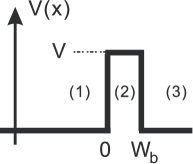
Figure 1: Schematics of the potential V(x) of a single square barrier.

The transfer matrix $N$ for this $\delta$-function barrier is calculated in appendix B and the limits $V\rightarrow\infty$ and $W_{b}\rightarrow 0$ are taken such that $P=VW_{b}/\hbar v_{F}$ is kept constant.

The transmission $T=|t|^{2}$ for $\alpha$ real and $\beta$ imaginary is obtained from the inverse amplitude,

$$\frac{1}{t}=\cos P+i\mu\sin P+\frac{(\alpha-\beta)^{2}k_{y}^{2}}{4\alpha\beta\varepsilon^{2}}\frac{\sin^{2}P}{\cos P+i\nu\sin P},$$ (7)

where $\mu=(\varepsilon+1/2)/\alpha$ and $\nu=(\varepsilon-1/2)/\beta$. Contour plots of the transmission $T$ are shown in Figs. 2(a) and 2(b) for strengths $P=0.25\pi$ and $P=0.75\pi$, respectively.

The transmission remains invariant under the transformations:

$$1) P\to P+n\pi,$$ (8)

$$2) k_{y}\to-k_{y}\,.$$

The first property is in contrast with what is obtained in Ref. kats, . In the latter work it was found, by using the $2\times 2$ Hamiltonian, that the transmission $T$ should be zero for $k_{y}\approx 0$ and $E<V_{0}$, while we can see here that for certain strengths $P=n\pi$ there is perfect transmission. The last property is due to the fact that $k_{y}$ only appears squared in the expression for the transmission. Notice that in contrast to single-layer graphene the transmission for $\varepsilon\approx 0$ is practically zero. The cone for nonzero transmission shifts to $\varepsilon=1/2(1-\cos P)$ with increasing $P$ till $P=\pi$. An area with $T=0$ appears when $\alpha$ is imaginary, i.e., for $\varepsilon^{2}+\varepsilon-k_{y}^{2}<0$ (as no propagating states are available in this area, we expect bound states to appear). From Figs. 2(a), 2(b) it is apparent that the transmission in the forward direction, i.e., for $k_{y}\approx 0$, is in general smaller than $1$; accordingly, there is no Klein tunneling. However, for $P=n\pi$, with $n$ an integer, the barrier becomes perfectly transparent.

For $P=n\pi$ we have $V=\hbar v_{F}(n\pi/W_{b})$. If the electron wave vector is $k=n\pi/W_{b}$ its energy equals the height of the potential barrier and consequently there is a quasi-bound state and thus a resonance matQdot . The condition on the wave vector implies $W_{b}=n\lambda/2$ where $\lambda$ is the wavelength. This is the standard condition for Fabry-Perot resonances. Notice though that the invariance of the transmission under the change $P\rightarrow P+n\pi$ is not equivalent to the Fabry-Perot resonance condition.

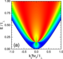
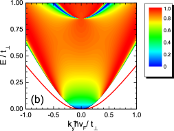
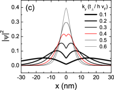
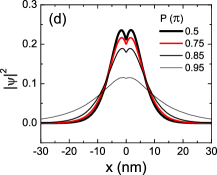
Figure 2: (Color online) Contour plot of the transmission for $P=0.25\pi$ in (a) and $P=0.75\pi$ in (b). In (b) the bound state, shown by the red curve, is at positive energy. The white area shows the part where $\alpha$ is imaginary. The probability distribution $|\psi(x)|^{2}$ of the bound state is plotted in (c) for various values of $k_{y}$ and in (d) for different values of $P$.

From the transmission we can calculate the conductance $G$ given, at zero temperature, by

$$G/G_{0}=\int_{-\pi/2}^{\pi/2}T(E,\phi)\cos\phi\mathrm{d}\phi,$$ (9)

where $G_{0}=(4e^{2}/2\pi h)[E_{F}^{2}+t_{\perp}E_{F}]^{1/2}/\hbar v_{F}$; the angle of incidence $\phi$ is determined by $\tan\phi=k_{y}/\alpha$. It is not possible to obtain the conductance analytically, therefore we evaluate this integral numerically.

The conductance is a periodic function of $P$ (since the transmission is) with period $\pi$. Fig. 3 shows a contour plot of the conductance for one period. As seen,

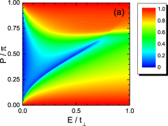
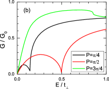
Figure 3: (Color online) (a) Contour plot of the conductance $G$. (b) Slices of $G$ along constant $P$.

the conductance has a sharp minimum at $\varepsilon=1/2(1-\cos P)$: this is due to the cone feature in the transmission which shifts to higher energies with increasing $P$. Such a sharp minimum was not present in the conductance of single-layer graphene when applied to the same $\delta$-function potential barrierbarb3 .

IV Bound states of a single $\delta$-function barrier

The bound states here are states that are localised in the x-direction close to the barrier but are free to move along the barrier, i.e. in the y-direction. Such bound states are characterised by the fact that the wave function decreases exponentially in the $x$ direction, i.e., the wave vectors $\alpha$ and $\beta$ are imaginary. This leads to

$$\begin{pmatrix}e_{g1}\\ 0\\ e_{g2}\\ 0\end{pmatrix}=\mathcal{N}\begin{pmatrix}0\\ e_{d1}\\ 0\\ e_{d2}\end{pmatrix},$$ (10)

which we can write as

$$\begin{pmatrix}0\\ 0\\ 0\\ 0\end{pmatrix}=\mathcal{Q}\begin{pmatrix}e_{d1}\\ e_{g1}\\ e_{d2}\\ e_{g2}\end{pmatrix},$$ (11)

where the matrix $\mathcal{Q}$ is the same as in Eq. (6). In order for this homogeneous algebraic set of equations to have a nontrivial solution, the determinant of $\mathcal{Q}$ must be zero. This gives rise to a transcendental equation for the dispersion relation

$$\det\mathcal{Q}=N_{11}N_{33}-N_{13}N_{31}=0,$$ (12)

which can be written explicitly

$$[\cos P+i\mu\sin P][\cos P+i\nu\sin P]+\frac{(\alpha-\beta)^{2}k_{y}^{2}}{4\alpha\beta\varepsilon^{2}}\sin^{2}P=0,$$ (13)

This expression is invariant under the transformations

$$1) P\rightarrow P+n\pi,$$ (14)

$$2) k_{y}\rightarrow-k_{y},$$

$$3) (\varepsilon,P)\rightarrow(-\varepsilon,\pi-P)\,.$$

Furthermore, there is one bound state for $k_{y}>0$ and $\pi/2<P<\pi$. For $P<\pi/2$ we can see that there is also a single bound state for negative energies from the third property above. From this transcendental formula one can find the solution for the energy $\varepsilon$ as function of $k_{y}$ numerically. We show the bound state by the solid red curve in Fig. 2(b). This state is bound to the potential in the $x$ direction but moves as a free particle in the $y$ direction. We have two such states, one that moves along the $+y$ direction and one along the $-y$ direction. The numerical solution approximates the curve $\varepsilon=\cos P\,[-1/2+(1/4+k_{y}^{2})^{1/2}]$. If one uses the $2\times 2$ Hamiltonian one obtains the dispersion relation given in Appendix C by Eq. (43). By solving this equation one finds for each value of $P$ two bound states one for positive and one for negative $k_{y}$. Moreover, for positive $P$ these bands have a hole like behaviour and for negative $P$ an electron like behaviour. Only for small $P$ do these results coincide with those from the $4\times 4$ Hamiltonian.

The wave function $\psi(x)$ of such a bound state is characterised by the coefficients $e_{g1}$, $e_{g2}$ on the left, and $e_{d1}$ and $e_{d2}$ on the right side of the barrier. We can obtain the latter coefficients by using Eq. (11), by assuming $e_{g1}=1$ and afterwards normalising the total probability to unity in dimensionless units. The wave function $\psi(x)$ to the left and right of the barrier can be determined from these coefficients by using Appendix A. In Figs. 2(c), (d) we show the probability distribution $|\psi(x)|^{2}$ of a bound state for a single $\delta$-function barrier: in (c) we show it for several $k_{y}$ values and in (d) for different values of $P$. One can see that the bound state is localised around the barrier and is less smeared out with increasing $k_{y}$. Notice that the bound state is more strongly confined for $P=\pi/2$ and that $|\psi(x)|^{2}$ is invariant under the transformation $P\rightarrow\pi-P$.

V Transmission through two $\delta$-function barriers

We consider a system of two barriers, separated by a distance $L$, with strengths $P_{1}$ and $P_{2}$, respectively, as shown schematically in Fig. 4. We have $L\rightarrow Lt_{\perp}/\hbar v_{F}\equiv 0.59261L/nm$ which for $L=10$ nm, $v_{F}=10^{6}$ m/s, and $t_{\perp}=0.39$ eV equals $5.9261$ in dimensionless units. The wave functions in the different regions are related as follows

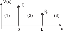
Figure 4: A system of two $\delta$-function barriers with strengths $P_{1}$ and $P_{2}$ placed a distance $L$ apart.

$$\psi_{1}(0) = \mathcal{S}_{1}\psi_{2}(0),\quad\psi_{2}(0)=\mathcal{S}^{\prime}\psi_{2}(L),$$

$$\psi_{2}(1) = \mathcal{S}_{2}\psi_{3}(L),\quad\psi_{1}(0)=\mathcal{S}_{1}\mathcal{S}^{\prime}\mathcal{S}_{2}\psi_{3}(L),$$ (15)

where $\mathcal{S}^{\prime}=\mathcal{G}\mathcal{M}(1)\mathcal{G}^{-1}$ represents a shift from x=0 to x=L and the matrices $S_{1}$ and $S_{2}$ are equal to the matrix $\mathcal{N}^{\prime}$ of Eq. (42) with $P=P_{1}$ and $P=P_{2}$, respectively. Using the transfer matrix $\mathcal{N}=\mathcal{G}^{-1}\mathcal{S}_{1}\mathcal{S}^{\prime}\mathcal{S}_{2}\mathcal{G}\mathcal{M}(L)$ we obtain the transmission $T=|t|^{2}$.

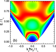
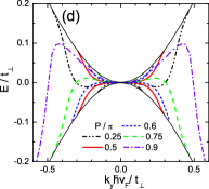
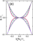
Figure 5: (Color online) Panels (a), (b), and (c): contour plots of the transmission through two $\delta$-function barriers of equal strength $P=|P_{1}|=|P_{2}|$ separated by a distance $L=10$ nm. For parallel barriers we took $P=0.25\pi$ in (a) and $P=0.5\pi$ in (b). For anti-parallel barriers results are given for $P=0.5\pi$ in (b) and $P=0.25\pi$ in (c). The solid red curves in the white background region is the spectrum for the bound states. Panels (d) and (e) show the dispersion relation of the bound states for various strengths $|P|$, respectively, for parallel and anti-parallel barriers. The thin black curves delimit the region where bound states are possible.

In Fig. 5 the transmission $T(\varepsilon,\,k_{y})$ is shown for parallel (a), (b) and anti-parallel (b), (c) $\delta$-function barriers with equal strength, i.e., for $|P_{1}|=|P_{2}|$, that are separated by $L=10$ nm, with $P=0.25\pi$ in (a) and $P=0.5\pi$ in (b). For $P=\pi/2$, the transmission amplitude $t$ for parallel barriers equals $-t$ for anti-parallel ones and the transmission $T$ is the same, as well the formula for the bound states. Hence panel (b) is the same for parallel and anti-parallel barriers. The contour plot of the transmission has a very particular structure which is very different from the single-barrier case. There are two bound states for each sign of $k_{y}$, which are shown in panel (d) for parallel and panel (e) for anti-parallel barriers. For anti-parallel barriers these states have mirror-symmetry with respect to $\varepsilon=0$ but for parallel barriers this symmetry is absent. For parallel barriers the change $P\rightarrow\pi-P$ will flip the spectrum of the bound state. The spectrum of the bound states extends into the low-energy transmission region and gives rise to a pronounced resonance. Notice that for certain $P$ values (Figs. 5(a) and 5(d)) the energy dispersion for the bound state has a camelback shape for small $k_{y}$, indicating free propagating states along the $y$ direction with velocity opposite to that for larger $k_{y}$ values. Contrasting Fig. 2(b) with Fig. 5(d)-(e)we see that the free-particle like spectrum of Fig. 2(b) for the bound states of a single $\delta$-function barrier is strongly modified when two $\delta$-function barriers are present.

From the transfer matrix we find that the transmission is invariant under the change $P\rightarrow P+n\pi$ and $k_{y}\rightarrow-k_{y}$ for parallel barriers, which was also the case of a single barrier, cf. Eq. (14). In addition, it is also invariant, for anti-parallel barriers, under the change

$$P\to\pi-P.$$ (16)

The conductance $G$ is calculated numerically as in the case of a single barrier. We show it for (anti-)parallel $\delta$-function barriers of equal strengths in Fig. 6. The symmetry $G(P+n\pi)=G(P)$ of the single barrier conductance holds here as well. Further, we see that for anti-parallel barriers $G$ has the additional symmetry $G(P)=G(\pi-P)$ as the transmission does.

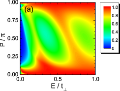
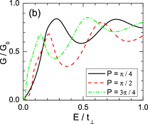
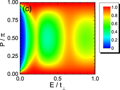
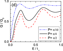
Figure 6: (Color online) Contour plot of the conductance of two $\delta$-function barriers with strength $|P_{2}|=|P_{1}|=P$ and inter-barrier distance $L=10$ nm. Panel (a) is for parallel barriers and panel (c) for anti-parallel barriers. Panels (b) and (d) show the conductance, along constant $P$, extracted from panels (a) and (c), respectively.

VI Kronig-Penney model

We consider an infinite sequence of equidistant $\delta$-function potential barriers, i.e., a superlattice (SL), with potential

$$V(x)=P\sum_{n}\delta(x-nL).$$ (17)

As this potential is periodic the wave function should be a Bloch function. Further, we know how to relate the coefficients $\mathcal{A}_{1}$ of the wave function before the barrier with those ($\mathcal{A}_{3}$) after it, see Appendix B. The result is

$$\psi(L)=e^{ik_{x}L}\psi(0),\quad\mathcal{A}_{1}=\mathcal{N}\mathcal{A}_{3},$$ (18)

with $k_{x}$ the Bloch wave vector. From these boundary conditions we can extract the relation

$$e^{-ik_{x}L}\mathcal{M}(L)\mathcal{A}_{3}=\mathcal{N}\mathcal{A}_{3},$$ (19)

with the matrix $\mathcal{M}(x)$ given by Eq. (36). The determinant of the coefficients in Eq. (19) must be zero, i.e.,

$$\det[e^{-ik_{x}L}\mathcal{M}(L)-\mathcal{N}]=0.$$ (20)

If $k_{y}=0$, which corresponds to the pure 1D case, one can easily obtain the dispersion relation because the first two and the last two components of the wave function decouple. Two transcendental equations are found

$$\cos k_{x}L=\cos\alpha L\cos P+\frac{1}{2}\left(\frac{\alpha}{\varepsilon}+\frac{\varepsilon}{\alpha}\right)\sin\alpha L\sin P,$$ (21a)

$$\cos k_{x}L=\cos\beta L\cos P+\frac{1}{2}\left(\frac{\beta}{\varepsilon}+\frac{\varepsilon}{\beta}\right)\sin\beta L\sin P.$$ (21b)

Since $\beta$ is imaginary for $0<E<t_{\perp}$, we can write Eq. (21b) as

$$\cos k_{x}L=\cosh|\beta|L\cos P-\frac{|\beta|^{2}+\varepsilon^{2}}{2|\beta|\varepsilon}\sinh|\beta|L\sin P,$$ (22)

which makes it easier to compare with the spectrum of the KP model obtained from the $2\times 2$ Hamiltonian, see Eq. (3). The latter is given by the two relations

$$\cos k_{x}L = \cos\kappa L+(P/2\kappa)\sin\kappa L,$$ (23a)

$$\cos k_{x}L = \cosh\kappa L-(P/2\kappa)\sinh\kappa L,$$ (23b)

with $\kappa=\sqrt{\varepsilon}$. This dispersion relation, which has the same form as the one for standard electrons, is not periodic in $P$ and the difference from that of the four-band Hamiltonian is due to the fact that the former is not valid for high potential barriers. One can also contrast the dispersion relations (21) and (23) with the corresponding one on single-layer graphene barb3

$$\cos k_{x}L=\cos\lambda L\cos P+\sin\lambda L\sin P,$$ (24)

where $\lambda=E/(\hbar v_{F})$. This dispersion relation is also periodic in $P$.

In Fig. 7 we plot slices of the energy spectrum for $k_{y}=0$. There is a qualitative difference, between the four-band and the two-band approximation for $P=\pi$. Only when $P$ is small does the difference between the two 1D dispersion relations become small. Therefore, we will no longer present results from the $2\times 2$ Hamiltonian though it has been used frequently due to its simplicity. The present results indicate that one should be very careful when using the $2\times 2$ Hamiltonian in bilayer graphene.

Notice that for $P=0.25\pi$ the electron and hole bands overlap and cross each other close to $|k_{y}|\approx 0.5(\pi/L)$. That is, this is the spectrum of a semi-metal. These crossing points move to the edge of the Brillouin zone (BZ) for $P=\pi$ resulting in a zero-gap semiconductor. At the edge of the BZ the spectrum is parabolic for low energies.

For $k_{y}\neq 0$, the dispersion relation can be written explicitly in the form

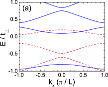
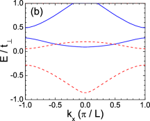
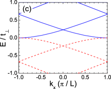
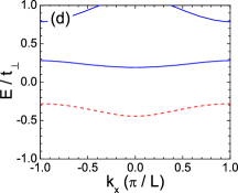
Figure 7: (Color online) Slices of the spectrum of a KP SL with $L=10$ $nm$ along $k_{x}$, for $k_{y}=0$, with $P=0.25\pi$ in (a) and (b) and $P=\pi$ in (c) and (d). The results in (a) and (c) are obtained from the four-band Hamiltonian (1) and those in (b) and (d) from the two-band one (3). The solid and dashed curves originate, respectively, from Eqs. (21a,23a) and (21b,23b).

$$\cos 2k_{x}L+C_{1}\cos k_{x}L+C_{0}/2=0,$$ (25)

where

$$C_{1}=-2(\cos\alpha L+\cos\beta L)\cos P-\left(d_{\alpha}+d_{\beta}\right)\sin P,$$ (26)

and

$$C_{0} = (2+k_{y}^{2}/\varepsilon^{2})+(2-k_{y}^{2}/\varepsilon^{2})\cos\alpha L\cos\beta L$$ (27)

$$+ [(\varepsilon^{2}-k_{y}^{2})^{2}+\varepsilon^{2}(2\varepsilon^{2}-1)]\sin\alpha L\sin\beta L/2\alpha\beta\varepsilon^{2}$$

$$- \Big{\{}k_{y}^{2}/\varepsilon^{2}-(2+k_{y}^{2}/\varepsilon^{2})\cos\alpha L\cos\beta L$$

$$+ \left[2\varepsilon^{2}-1/2-k_{y}^{2}+k_{y}^{4}/\varepsilon^{2}\right]\sin\alpha L\sin\beta L/\alpha\beta\Big{\}}\cos 2P$$

$$+ \left[d_{\alpha}\cos\beta L+d_{\beta}\cos\alpha L\right]\sin 2P,$$

with $d_{\alpha}=(2\varepsilon+1)\sin\alpha L/\alpha$ and $d_{\beta}=(2\varepsilon-1)\sin\beta L/\beta$. The wave vectors $\alpha=[\varepsilon^{2}+\varepsilon-k_{y}^{2}]^{1/2}$ and $\beta=[\varepsilon^{2}-\varepsilon-k_{y}^{2}]^{1/2}$ are pure real or imaginary. If $\beta$ becomes imaginary, the dispersion relation is still real ($\beta\rightarrow i|\beta|$ and $\sin\beta L\rightarrow i\sinh|\beta|L$). Further, if $\alpha$ becomes imaginary, that is for $\alpha\rightarrow i|\alpha|$, the dispersion relation is real. The dispersion relation has the following invariance properties:

$$1)\,E(k_{x},k_{y},P) = E(k_{x},k_{y},P+2n\pi),$$ (28a)

$$2)\,E(k_{x},k_{y},P) = -E(\pi/L-k_{x},k_{y},\pi-P),$$ (28b)

$$3)\,E(k_{x},k_{y},P) = E(k_{x},-k_{y},P).$$ (28c)

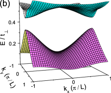
Figure 8: (Color online) SL Spectrum for $L=10$ nm, the lowest conduction and highest valence band for $P=0.25\pi$ in (a) and $P=0.5\pi$ in (b), are shown.

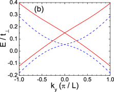
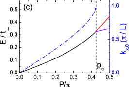
Figure 9: (Color online) SL spectrum for $L=10$ $nm$. The dashed blue, solid red, and dash-dotted purple curves are, respectively, for strengths $P=0.1\pi$, $P=0.25\pi$, and $P=0.5\pi$. (a) shows the spectrum vs $k_{x}$ for $k_{y}=0$ while (b) shows it vs $k_{y}$ for $k_{x}$ at the value where the bands cross. The position of the touching points and the size of the energy gap are shown in (c) as a function of $P$. The dash-dotted, blue curve and the solid, black curve show $k_{x,0}$ and the energy value of the touching points, respectively. For $P>P_{c}$ a gap appears; the energies of the conduction band minimum and of the valence band maximum are shown by the red and purple, solid curve, respectively.

In Fig. 8 we show the lowest conduction and highest valence bands of the energy spectrum of the KP model for $P=0.25\pi$ in (a) and $P=0.5\pi$ in (b). The former has two touching points which can also be viewed as overlapping conduction and valence bands as in a semi-metal and the latter exhibits an energy gap. In Fig. 9 slices of Figs. 8(a), (b) are plotted for $k_{y}=0$. The spectrum of bilayer graphene has a single touching point at the origin. When the strength $P$ is small, this point shifts away from zero energy along the $k_{x}$ axis with $k_{y}=0$ and splits into two points. It is interesting to know when and where these touching points emerge. To find out we observe that at the crossing point both relations (21) should be fulfilled. If these two relations are subtracted we obtain the transcendental equation

$$0=(\cos\alpha L-\cos\beta L)\cos P+(1/2)\left(d_{\alpha}-d_{\beta}\right)\sin P,$$ (29)

where $d_{\alpha}=(2\varepsilon+1)\sin\alpha L/\alpha$ and $d_{\beta}=(2\varepsilon-1)\sin\beta L/\beta$. We can solve Eq. (28) numerically for the energy $\varepsilon$. For small $P$ and small $L$ this energy can be approximated by $\varepsilon=P/L$. Afterwards we can put this solution back into one of the dispersion relations to obtain $k_{x}$.

In Figs. 9(a), (b) we show slices along the $k_{x}$ axis for $k_{y}=0$ and along the $k_{y}$ axis for the $k_{x}$ value of a touching point, $k_{x,0}$. We see that as the touching points move away from the $K$ point, the cross sections show a more linear behaviour in the $k_{y}$ direction. The position of the touching points is plotted in Fig. 9(c) as a function of $P$. The dash-dotted blue curve corresponds to the value of $k_{x,0}$ (right $y$ axis), while the energy value of the touching point is given by the black solid curve. This touching point moves to the edge of the BZ which occurs for $P=P_{c}\approx 0.425\pi$. At this point a gap opens (the energies of the top of the valence band and of the bottom of the conduction band are shown by the lower purple and upper red solid curve, respectively) and increases with $P$. Because of property 2) in Eq. 28(b) we plot the results only for $P<\pi/2$. We draw attention to the fact that the dispersion relation differs to large extent for large $P$ from the one that results from the $2\times 2$ Hamiltonian given in Appendix C. This is already apparent from the fact that the dispersion relation does not exhibit any of the periodic in $P$ behaviours given by Eqs. (28a) and (28b).

An important question is whether the above periodicities in $P$ still remain approximately valid outside the range of validity of the KP model. To assess that we briefly look at a square-barrier SL with barriers of finite width $W_{b}$ and compare the spectra with those of the KP model. We assume the height of the barrier to be $V/\hbar v_{F}=P/W_{b}$, such that $VW_{b}/\hbar v_{F}=P$. The SL period we use is $50$ nm and the width $W_{b}=0.05L=2.5$ nm. For $P=\pi/2$ the corresponding height is then $V\approx t_{\perp}$. To fit in the continuum model we require that the potential barriers be smooth over the carbon-carbon distance which is $a\approx 0.14$ nm. In Fig. 10 we show the spectra for the KP model and this SL. Comparing (a) and (b) we see that for $P$ small the difference between both models is rather small. If we take $P=\pi/2$ though, this difference becomes large, especially for the first conduction and valence minibands, as shown in panels (c) and (d). The latter energy bands are flat for large $k_{y}$ in the KP model, while they diverge from the horizontal line (E=0) for a finite barrier width. From panel (f), which shows the discrepancy of the SL minibands between the exact ones and those obtained from the KP model, we see that the spectra with $P=0.2\pi$ are closer to the KP model than those for $P=\pi/2$. Fig. 10(e) demonstrates that the periodicity of the spectrum in $P$ within the KP model, i.e., its invariance under the change $P\rightarrow P+2n\pi$, is present only as a rough approximation away from it.

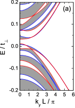
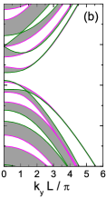
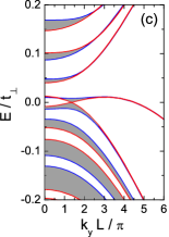
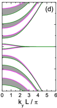
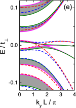
Figure 10: (Color online) Spectrum of a SL with $L=50$ nm, (a) and (b) are for $P=0.2\pi$ and (c) and (d) are for $P=\pi/2$. (a), (c) and (e) are for a rectangular-barrier SL with $W_{b}=0.05L$ and $u=P/W_{b}$, while (b) and (d) are for the KP model. (e) shows the spectrum for $u$ corresponding to $P=(1/2+2)\pi$; the dashed curves show the contours of the spectrum in (c) for $P=\pi/2$. (f) Shows the discrepancy of the SL minibands between the exact ones and those obtained from the KP model, averaged over k space (where we used $k_{y}L/\pi=6$ as a cut-off). The conduction (valence) minibands are numbered with positive (negative) integers.

VII Extended Kronig-Penney model

In this model we replace the single $\delta$-function barrier in the unit cell by two barriers with strengths $P_{1}$ and $-P_{2}$. Then the SL potential is given by

$$V(x)=P_{1}\sum_{n}\delta(x-nL)-P_{2}\sum_{n}\delta(x-(n+1/2)L).$$ (30)

Here we will restrict ourselves to the important case of $P_{1}=P_{2}$. For this potential we can also use Eq. (20) of Sec. VI, with the transfer matrix $\mathcal{N}$ replaced by the appropriate one of Sec. V.

First, let us consider the spectrum along $k_{y}=0$ which is determined by the transcendental equations

$$\cos k_{x}L = \cos\alpha L\cos^{2}P+D_{\alpha}\sin^{2}P,$$ (31a)

$$\cos k_{x}L = \cos\beta L\cos^{2}P+D_{\beta}\sin^{2}P,$$ (31b)

with $D_{\gamma}=\left[(\gamma^{2}+\varepsilon^{2})\cos\gamma L-\gamma^{2}+\varepsilon^{2}\right]/4\gamma^{2}\varepsilon^{2}$. It is more convenient to look at the crossing points because the spectrum is symmetric around zero energy. This follows from the form of the potential (its spatial average is zero) or from the dispersion relation (31a): the change $\varepsilon\rightarrow-\varepsilon$ entails $\alpha\leftrightarrow\beta$ and the crossings in the spectrum are easily obtained by taking the limit $\varepsilon\rightarrow 0$ in one of the dispersion relations. This gives the value of $k_{x}$ at the crossings

$$k_{x,0}=\pm\arccos[1-(L^{2}/8)\sin^{2}P]/L,$$ (32)

and the crossing points are at $(\varepsilon,\,k_{x},\,k_{y})=(0,\,\pm k_{x,0},\,0)$. If the $k_{x,0}$ value is not real, then there is no solution at zero energy and a gap arises in the spectrum. From Eq. (31a) we see that for $\sin^{2}P>16/L^{2}$ a band gap arises.

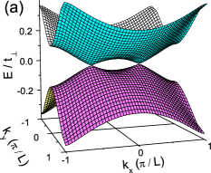
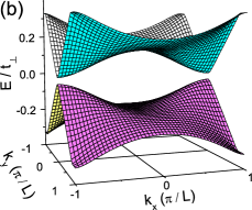
Figure 11: (Color online) The first conduction and valence minibands for the extended KP model for $L=10$ nm with $P=0.125\pi$ in (a) and $P=0.25\pi$ in (b).

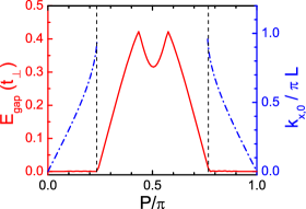
Figure 12: (Color online) Plot of the $\pm k_{x,0}$ values, for which the minibands touch each other, as a function of $P$ (dash-dotted, blue curve), and the size of the band gap $E_{gap}$ (solid, red curve). The calculation is done for the extended KP model with $L=10$ nm.

In Fig. 11 we show the lowest conduction and highest valence band for (a) $P=0.125\pi$, and (b) $P=0.25\pi$. If we make the correspondence with the KP model of Sec. V we see that this model leads to qualitatively similar (but not identical) spectra shown in Figs. 8(a) and 8(b): one should take $P$ twice as large in the corresponding KP model of Sec. V in order to have a similar spectrum. Here we have the interesting property that the spectrum exhibits mirror symmetry with respect to $\varepsilon=0$ which makes the analysis of the touching points and of the gap easier.

In Fig. 12 we plot the $k_{x}$ value (dash-dotted, blue curve) of the touching points $k_{x,0}$ versus $P$, if there is no gap, and the size of the gap $E_{gap}$ (solid, red curve) if there is one. The touching points move toward the BZ boundary with increasing $P$. Beyond the $P$ value for which the boundary is reached, a gap appears between the conduction and valence minibands.

VIII Conclusions

We investigated the transmission through single and double $\delta$-function potential barriers on bilayer graphene using the four-band Hamiltonian. The transmission and conductance are found to be periodic functions of the strength of the barriers $P=VW_{b}/\hbar v_{F}$ with period $\pi$. The same periodicity was previously obtained for such barriers on single-layer graphene barb3 . We emphasise that the periodicity obtained here implies that the transmission satisfies the relation $T(k_{x},k_{y},P)=T(k_{x},k_{y},P+n\pi)$ for arbitrary values of $k_{x}$, $k_{y}$, $P$, and integer $n$. In previous theoretical work on graphene svi and bilayer graphene been ; mass Fabry-Pérot resonances were studied and $T=1$ was found for particular values of $\alpha$, the electron momentum inside the barrier along the $x$ axis. For a rectangular barrier of width $W$ and Schrödinger-type electrons, Fabry-Pérot resonances occur for $\alpha W=n\pi$ and $E>V_{0}$ as well as in the case of a quantum well for $E>0$, $V_{0}<0$. In graphene, because of Klein tunnelling, the latter condition on energy is not needed. Because $\alpha$ depends on the energy and the potential barrier height in the combination $E-V_{0}$, any periodicity of $T$ in the energy is equivalent to a periodicity in $V_{0}$ if no approximations are made, e.g., $E\ll V_{0}$, etc. Although this may appear similar to the periodicity in $P$, there are fundamental differences. As shown in Ref. been, , the Fabry-Pérot resonances are not exactly described by the condition $\alpha W=n\pi$ (see Fig. 3 in Ref. been, ) while the periodicity of $T$ in the effective barrier strength is exactly $n\pi$. Furthermore, the Fabry-Pérot resonances are found for $T=1$, while the periodicity of $T$ in $P$ is valid for any value of $T$ between $0$ and $1$.

Further, we studied the spectrum of the KP model and found it to be periodic in the strength $P$ with period $2\pi$. In the extended KP model this period reduces to $\pi$. This difference is a consequence of the fact that for the extended SL the unit cell contains two $\delta$-function barriers. These periodicities are identical to the one found earlier in the (extended) KP model on single-layer graphene. We found that the SL conduction and valence minibands touch each other at two points or that there is a energy gap between them. In addition, we found a simple relation describing the position of these touching points. None of these periodic behaviours results from the two-band Hamiltonian; this clearly indicates that the two-band Hamiltonian is an incorrect description of the KP model in bilayer graphene. In general, results derived from these two tight-binding Hamiltonians agree well only for small energies cast . The precise energy ranges are not explicitly known and may depend on the particular property studied. For the range pertaining to the four-band Hamiltonian ab-initio results lat indicate that it is approximately from $-1$ eV to + $0.6$ eV.

The question arises whether the above periodicities in $P$ survive when the potential barriers have a finite width. To assess that we briefly investigated the spectrum of a rectangular SL potential with thin barriers and compared it with that in the KP limit. We showed with some examples that for specific SL parameters the KP model is acceptable in a narrow range of $P$ and only as a rough approximation away from this range. The same conclusion holds for the periodicity of the KP model.

The main differences between the results of this work and those of our previous one, Ref. barb3, , are as follows. In contrast to monolayer graphene we found here that:
1) The conductance for a single $\delta$-function potential barrier depends on the Fermi energy and drops almost to zero for certain values of $E$ and $P$. 2) The KP model (and its extended version) in bilayer graphene can open a band gap; if there is no such gap, two touching points appear in the spectrum instead of one. 3) The Dirac line found in the extended KP model in single-layer graphene is not found in bilayer graphene.

Appendix A Eigenvalues and eigenstates for a constant potential

Starting with the Hamiltonian (1) for a one-dimensional potential $V(x,y)=V(x)$, the time-independent Schrödinger equation $\mathcal{H}\psi=E\psi$ leads to

$$-i(\partial_{x}-k_{y})\psi_{B} =\varepsilon^{\prime}\psi_{A}-\psi_{B^{\prime}},$$ (33)

$$-i(\partial_{x}+k_{y})\psi_{A} =\varepsilon^{\prime}\psi_{B},$$

$$-i(\partial_{x}+k_{y})\psi_{A^{\prime}} =\varepsilon^{\prime}\psi_{B^{\prime}}-\psi_{A},$$

$$-i(\partial_{x}-k_{y})\psi_{B^{\prime}} =\varepsilon^{\prime}\psi_{A^{\prime}},$$

The spectrum and the corresponding eigenstates can be obtained, for constant $V(x,y)=V$, by progressive elimination of the unknowns in Eq. (33) and solution of the resulting second-order differential equations. The result for the spectrum is

$$\varepsilon =u+1/2\pm\sqrt{1/4+k^{2}},$$ (34)

$$\varepsilon =u-1/2\pm\sqrt{1/4+k^{2}}.$$

The unnormalised eigenstates are given by the columns of the matrix $\mathcal{G}\mathcal{M}$, where

$$\mathcal{G}=\begin{pmatrix}1&1&1&1\\ f^{\alpha}_{+}&f^{\alpha}_{-}&f^{\beta}_{+}&f^{\beta}_{-}\\ -1&-1&1&1\\ f^{\alpha}_{-}&f^{\alpha}_{+}&-f^{\beta}_{-}&-f^{\beta}_{+}\\ \end{pmatrix},$$ (35)

with $f^{\alpha,\beta}_{\pm}=-i(k_{y}\pm i{(\alpha,\beta)})/\varepsilon^{\prime}$; $\alpha=[\varepsilon^{\prime 2}+\varepsilon^{\prime}-k_{y}^{2}]^{1/2}$ and $\beta=[\varepsilon^{\prime 2}-\varepsilon^{\prime}-k_{y}^{2}]^{1/2}$ are the wave vectors. $\mathcal{M}$ is given by

$$\mathcal{M}=\begin{pmatrix}e^{i\alpha x}&0&0&0\\ 0&e^{-i\alpha x}&0&0\\ 0&0&e^{i\beta x}&0\\ 0&0&0&e^{-i\beta x}\\ \end{pmatrix}.$$ (36)

The wave function in a region of constant potential is a linear combination of the eigenstates and can be written

$$\Psi(x)=\begin{pmatrix}\psi_{A}\\ \psi_{B}\\ \psi_{B^{\prime}}\\ \psi_{A^{\prime}}\end{pmatrix}=\mathcal{G}\mathcal{M}\begin{pmatrix}A\\ B\\ C\\ D\end{pmatrix}.$$ (37)

We can reduce its complexity by the linear transformation $\Psi(x)\to\mathcal{R}\Psi(x)$ where

$$\mathcal{R}=\frac{1}{2}\begin{pmatrix}1&0&-1&0\\ 0&1&0&-1\\ 1&0&1&0\\ 0&1&0&1\\ \end{pmatrix},$$ (38)

which transforms $\Psi(x)$ to $\Psi(x)=(1/2)(\psi_{A}-\psi_{B^{\prime}},\,\psi_{B}-\psi_{A^{\prime}},\,\psi_{A}+\psi_{B^{\prime}},\,\psi_{B}+\psi_{A^{\prime}})^{T}$. Then the basis functions are given by the columns of $\mathcal{G}\mathcal{M}$ with

$$\mathcal{G}=\begin{pmatrix}1&1&0&0\\ \alpha/\varepsilon^{\prime}&-\alpha/\varepsilon^{\prime}&-ik_{y}/\varepsilon^{\prime}&-ik_{y}/\varepsilon^{\prime}\\ 0&0&1&1\\ -ik_{y}/\varepsilon^{\prime}&-ik_{y}/\varepsilon^{\prime}&\beta/\varepsilon^{\prime}&-\beta/\varepsilon^{\prime}\\ \end{pmatrix}.$$ (39)

The matrix $\mathcal{M}$ is unchanged under the transformation $\mathcal{R}$ and the new $\Psi(x)$ fulfils the same boundary conditions as the old one.

Appendix B The transfer matrix

We denote the wave function to the left of, inside, and to the right of the barrier by $\psi_{j}(x)=\mathcal{G}_{j}\mathcal{M}_{j}\mathcal{A}_{j}$, with $j=1$, $2$, and $3$, respectively. Further, we have $\mathcal{G}_{1}=\mathcal{G}_{3}$ and $\mathcal{M}_{1}=\mathcal{M}_{3}$. The continuity of the wave function at $x=0$ and $x=W_{b}$ gives the boundary conditions $\psi_{1}(0)=\psi_{2}(0)$ and $\psi_{2}(W_{b})=\psi_{3}(W_{b})$. In explicit matrix notation this gives $\mathcal{G}_{1}\mathcal{A}_{1}=\mathcal{G}_{2}\mathcal{A}_{2}$ and $\mathcal{G}_{2}\mathcal{M}_{2}(W_{b})\mathcal{A}_{2}=\mathcal{M}_{1}(W_{b})\mathcal{G}_{1}\mathcal{A}_{3}$, where $\mathcal{A}_{1}=\mathcal{G}_{1}^{-1}\mathcal{G}_{2}\mathcal{M}^{-1}_{2}(W_{b})\mathcal{G}^{-1}_{2}\mathcal{G}_{1}\mathcal{M}_{1}(W_{b})\mathcal{A}_{3}$. Then the transfer matrix $\mathcal{N}$ can be written as $\mathcal{N}=\mathcal{G}_{1}^{-1}\mathcal{G}_{2}\mathcal{M}^{-1}_{2}(W_{b})\mathcal{G}^{-1}_{2}\mathcal{G}_{1}\mathcal{M}_{1}(W_{b})$. Let us define $\mathcal{N}^{\prime}=\mathcal{G}_{2}\mathcal{M}^{-1}_{2}(W_{b})\mathcal{G}^{-1}_{2}$, which leads to $\psi_{1}(0)=\mathcal{N}^{\prime}\psi_{3}(W_{b})$.

To treat the case of a $\delta$-function barrier we take the limits $V\rightarrow\infty$ and $W_{b}\rightarrow 0$ such that the dimensionless potential strength $P=VW_{b}/\hbar v_{F}$ is kept constant. Then $\mathcal{G}_{2}$ and $\mathcal{M}_{2}(W_{b})$ simplify to

$$\mathcal{G}_{2}=\begin{pmatrix}1&1&0&0\\ -1&1&0&0\\ 0&0&1&1\\ 0&0&-1&1\end{pmatrix},$$ (40)

$$\mathcal{M}_{2}(W_{b})=\begin{pmatrix}e^{iP}&0&0&0\\ 0&e^{-iP}&0&0\\ 0&0&e^{iP}&0\\ 0&0&0&e^{-iP}\end{pmatrix},$$ (41)

and $\mathcal{N}^{\prime}$ becomes

$$\mathcal{N}^{\prime}=\begin{pmatrix}\cos P&i\sin P&0&0\\ i\sin P&\cos P&0&0\\ 0&0&\cos P&i\sin P\\ 0&0&i\sin P&\cos P\end{pmatrix}.$$ (42)

Appendix C Results for the $2\times 2$ Hamiltonian

Using the $2\times 2$ Hamiltonian (3) instead of the $4\times 4$ one can sometimes lead to unexpectedly different results; below we give a few examples. In a slightly modified notation pertinent to the $2\times 2$ Hamiltonian we set $\alpha=[-\varepsilon+k_{y}^{2}]^{1/2}$, $\beta=[\varepsilon+k_{y}^{2}]^{1/2}$, and use the same dimensionless units as before.

Bound states for a single $\delta$-function barrier $u(x)=P\delta(x)$, without accompanying propagating states, are possible if $k_{y}=0$ or $k_{y}^{2}>|\varepsilon|$. In the former case the single solution is $\varepsilon=-sign(P)P^{2}/4$. In the latter one the dispersion relation is

$$\varepsilon^{2}(P+2\alpha)(P-2\beta)+2P^{2}k_{y}^{2}(\alpha\beta-k_{y}^{2})=0.$$ (43)

The dispersion relation for the KP model obtained from the $2\times 2$ Hamiltonian is

$$\cos(2kL)+2F_{1}\cos(kL)+F_{2}=0,$$ (44)

where

$$F_{1}=-\cosh(\beta L)-\cosh(\alpha L)+\frac{P}{2\beta}\sinh(\beta L)-\frac{P}{2\alpha}\sinh(\alpha L),$$ (45)

$$F_{2}=\frac{1}{\alpha\beta\varepsilon^{2}}\left\{\alpha\beta(\varepsilon^{2}+k_{y}^{2}P^{2}/4)\right.$$

$$\quad+\beta\cosh(\beta L)\left[\alpha(2\varepsilon^{2}-k_{y}^{2})\cosh(\alpha L)+\varepsilon^{2}P\sinh(\alpha L)\right]$$

$$\left.\quad-\frac{P}{2}\sinh(\beta L)\left[\alpha(\varepsilon^{2}-k_{y}^{4}/2)P\sinh(\alpha L)+2\varepsilon^{2}\alpha\cosh(\alpha L)\right]\right\}.$$

References

- (1) K. S. Novoselov, A. K. Geim, S. V. Morozov, D. Jiang, Y. Zhang, S. V. Dubonos, I. V. Grigorieva, and A. A. Firsov, Science 306, 666 (2004).
- (2) O. Klein, Z. Phys. 53, 157 (1929).
- (3) M. I. Katsnelson, K. S. Novoselov, and A. K. Geim, Nature Physics 2, 620 (2006).
- (4) N. Stander, B. Huard, and D. Goldhaber-Gordon, Phys. Rev. Lett. 102, 026807 (2009); A. F. Young and P. Kim, Nature Phys. 5, 222 (2009).
- (5) A. H. Castro Neto, F. Guinea, N. M. R. Peres, K. S. Novoselov, and A. K. Geim, Rev. Mod. Phys. 81, 109 (2009); C. W. J. Beenakker, ibid 80, 1197 (2008).
- (6) J. M. Pereira Jr., P. Vasilopoulos, and F. M. Peeters, Appl. Phys. Lett. 90, 132122 (2007).
- (7) E. McCann, D. S. L. Abergel, and V. I. Fal’ko, Solid State Comm. 143, 110 (2007).
- (8) C.-H. Park, L. Yang, Y.-W. Son, M. L. Cohen, and S. G. Louie, Nature Phys. 4, 213 (2008).
- (9) S. Ghosh and M. Sharma, J. Phys.: Condens. Matter 21, 292204 (2009).
- (10) Y. P. Bliokh, V. Freilikher, S. Savel’ev, and F. Nori, Phys. Rev. B 79, 075123 (2009).
- (11) I. Snyman, Phys. Rev. B 80, 054303 (2009).
- (12) R. Nasir, K. Sabeeh, and M. Tahir, Phys. Rev. B 81, 085402 (2010).
- (13) M. Barbier, F. M. Peeters, P. Vasilopoulos, and J. M. Pereira Jr., Phys. Rev. B 77, 115446 (2008).
- (14) C. Bai and X. Zhang, Phys. Rev. B 76, 075430 (2007).
- (15) M. Barbier, P. Vasilopoulos, F. M. Peeters, and J. M. Pereira Jr., Phys. Rev. B 79, 155402 (2009).
- (16) C. Kittel, Introduction to Solid State Physics, 5th edn, (John Wiley & Sons, Inc., 1976).
- (17) M. Barbier, P. Vasilopoulos, and F. M. Peeters, Phys. Rev. B 80, 205415 (2009).
- (18) E. McCann and V. I. Fal’ko, Phys. Rev. Lett. 96, 086805 (2006).
- (19) A. Matulis and F. M. Peeters, Phys. Rev. B 77, 115423 (2008).
- (20) A. V. Shytov, M. S. Rudner, and L. S. Levitov, Phys. Rev. Lett. 101, 156804 (2008); P. G. Silvestrov and K. B. Efetov, ibid. 98, 016802 (2007); F. Young and Philip Kim, Nature Physics 5, 222 (2009).
- (21) I. Snyman and C. W. J. Beenakker, Phys. Rev. B 75, 045322 (2007).
- (22) M. Ramezani Masir, P. Vasilopoulos, and F. M. Peeters, Phys. Rev. B 82, 115417 (2010).
- (23) S. Latil and L. Henrard, Phys. Rev. Lett. 97, 036803 (2006).