Asymptotic Expansion for Multiscale Problems on Non-periodic Stochastic Geometries

Abstract.

The asymptotic expansion method is generalized from the periodic setting to stationary ergodic stochastic geometries. This will demonstrate that results from periodic asymptotic expansion also apply to non-periodic structures of a certain class. In particular, the article adresses non-mathematicians who are familiar with asymptotic expansion and aims at introducing them to stochastic homogenization in a simple way. The basic ideas of the generalization can be formulated in simple terms, which is basically due to recent advances in mathematical stochastic homogenization. After a short and formal introduction of stochastic geometry, calculations in the stochastic case will be formulated in a way that they will not look different from the periodic setting. To demonstrate that, the method will be applied to diffusion with and without microscopic nonlinear boundary conditions and to porous media flow. Some examples of stochastic geometries will be given.

1. Introduction

Homogenization has become an important modeling tool for multiscale problems, i.e. phenomena that have causes and effects on multiple spatial scales. The application ranges from Physics (porous media flow, freezing processes in porous media, erosion[2, 7, 22]), engineering (composite materials, reaction diffusion equations in catalysts[19, 11]) to biology (processes in tissue[13], membranes[20]). Also the numerical investigation of such problems is of interest (see [16] and references therein).

Homogenization considers physical, chemical or biological processes on large domains with a periodic microstructure of period $\varepsilon\ll 1$. On this periodic structure, a set of equations describing the several processes are set up and the limit behavior of the solutions of these equations is investigated as $\varepsilon\rightarrow 0$. Note that $\varepsilon\rightarrow 0$ is a mathematical equivalent of the assumption $\varepsilon\ll 1$, which means basically very small microstructures compared to the domain of interest. For example, one may think of a solid structure perforated by a periodic structure of channels, which are filled by a Newtonian fluid, i.e. a fluid whose motion is described by the Navier-Stokes equations. Since one is usually interested in a scale of meters and the pores have sizes of $mm$, it follows $\varepsilon\approx 10^{-3}$. In the limit $\varepsilon\rightarrow 0$, the velocity field would follow Darcy’s law [10] (see sections 2.2 and 4.2).

There are two ways to obtain the limit equations: Via strong mathematical calculations (proofs of convergence of solutions) or via rather formal calculations. One of the formal ways to obtain averaged equations is the so called asymptotic expansion. Its ansatz is to expand the solution in a series of functions multiplied with increasing powers of $\varepsilon$, where the functions in this expansion depend on a global variable and a periodic variable. We will demonstrate the basics of this approach below in section 2.

Strong mathematical investigations where originally based on strong and weak convergence methods in Sobolev spaces, which is nowadays still a method of choice. However, lots of other convergence methods entered homogenization theory such as $\Gamma$- and $G$-convergence, see [26] for an overview.

In the beginning of the 1990’s, Allaire and Nguetseng [21, 1] developed the so called two-scale convergence which was later extended by Neuss-Radu, Zhikov and Lukkassen and Wall [18, 25, 12]. As an interesting feature, two-scale convergence is related to an asymptotic expansion in the weak sense and therefore closely connected to the formal method. This similarity becomes even more striking by the method of periodic unfolding, developed by Cioranescu, Damlamian and Griso [5, 4], and which can be considered as a consequent generalization of two-scale convergence. In comparing the methods, one may get the idea that every result from formal asymptotic expansion could be proved rigorously. However, for many homogenization problems there are lots of technical difficulties like regularity proofs or a lack of Poincaré-inequalities which are sometimes to hard to be overcome.

There is, however, the justified criticism, that the methods above are based on the assumption of a periodic structure and that the resulting equations therefore may not be valid for a non-periodic medium. Nevertheless, we expect that many of the derived equations may also hold for non-periodic microscopic geometries: Darcy’s law is observed to hold in most porous media may it be sand, silt or loam. In a polycrystal or a composite material (industrial ceramics) with their complex microstructure, we assume that heat transport still follows Fourier’s law with averaged coefficients. Reaction diffusion equations derived for a catalyzer should also hold if the microscopic structure is not perfectly periodic.

So, it is an important question whether or not it is possible to apply homogenized results to non-periodic geometries and under what circumstances. Mathematicians were aware of this problem and tried to apply homogenization techniques to non-periodic structures. An overview over many results before 1994 can be found in [26].

In 2006, Zhikov and Piatnitsky [27] where able to introduce a two-scale convergence method on stationary, ergodic stochastic geometries on a compact probability space. Their results where generalized to arbitrary probability spaces by the author in [8]. A former attempt by Bourgeat, Mikelić and Wright [3] in the non-ergodic setting used an averaged form of two-scale convergence and was not applicable to problems on manifolds or complex boundary conditions. Also, due to the averaging, it was less close to the periodic setting than [27].

The results in [8] provide a geometrical interpretation of subsets of the probability space and demonstrates that all periodic quantities find their precise analogue in the stochastic case and vice versa. Moreover, if a stationary ergodic structure is periodic, the probability space has to be essentially the unit cell. The theory has been applied successfully to heat transfer in polycrystals in [9].

Due to the connection between two-scale convergence and asymptotic expansion in the periodic setting, these mathematical results give the basic idea to extend the asymptotic expansion to the stochastic case. Note that it is not the intention of this article, to give a rigorous mathematical introduction to stochastic geometry or stochastic homogenization. Rather it is the aim of this paper to demonstrate that it can be mathematically justified to apply results from asymptotic expansion to stochastic settings and that there is formally no difference in the calculations. The most important theoretical results are cited in the appendix. For proofs of the fundamental theorems which are cited in this article, the reader is referred to [27, 8] and the references therein.

This article is organized as follows: In the next section, the basic idea of periodic asymptotic expansion is explained and the resulting equations for two sample problems (diffusion and porous media flow) are given. In section 3, the concepts of stochastic geometry will be introduced in a formal and mathematical non rigorous way. The connections to periodic geometries are explained. In section 4 the asymptotic expansion on stochastic geometries will be introduced and applied to thermal diffusion, porous media flow and diffusion processes with reactions on the microscopic boundary. In section 5 some simple examples of stochastic geometries will be given.

2. Recapitulation of the Periodic Case

In this section we will shortly recapitulate the asymptotic expansion technique for periodic structures. It is not the intention of this section to go into the details of calculations but to rather explain what are the mathematical problems, the ansatz that people use to solve these problems and what the results look like. For both examples, precise calculations will follow in section 4 below. We will first consider the standard homogenization problem of diffusion (following [10]) and then discuss Navier-Stokes flow through porous media. In all calculations below and throughout the paper, $n$ denotes the dimension of space (in a physical setting $n=2$ or $n=3$).

2.1. The standard problem

Given an open and bounded set $\boldsymbol{Q}\subset\mathbb{R}^{n}$ investigate diffusion processes (for example heat diffusion) with a source term and rapidly oscillating coefficients which are due to a periodic microstructure. In particular, assume that for $\boldsymbol{Y}:=[0,1[^{n}$ we have $\boldsymbol{Y}=A\cup B\cup\Gamma$ with $A$, $B$ open in $\boldsymbol{Y}$ such that $A\cap B=\emptyset$ and $\Gamma=\partial A=\partial B$ in $\boldsymbol{Y}$. We expand $\boldsymbol{Y}$ periodically to $\mathbb{R}^{n}$ and identify $A$, $B$ and $\Gamma$ with their periodic continuation. We furthermore denote $A^{\varepsilon}=\varepsilon A$, $B^{\varepsilon}:=\varepsilon B$ and $\Gamma^{\varepsilon}:=\varepsilon\Gamma$. The diffusion constants in $A$ and $B$ are thought to be different.

The mathematical problem reads

$$\partial_{t}u^{\varepsilon}-\mbox{div}\,\left(D^{\varepsilon}\nabla u^{\varepsilon}\right) =f \mbox{on }]0,T]\times\boldsymbol{Q}$$

$$u^{\varepsilon} =0 \mbox{on }]0,T]\times\partial\boldsymbol{Q}$$

$$u^{\varepsilon}(0,\cdot) =a(\cdot) \mbox{on }\boldsymbol{Q}\mbox{ for }t=0$$

where $D^{\varepsilon}$ is given by $D^{\varepsilon}:=D(t,x,\frac{x}{\varepsilon})$ and $D$ is a $\boldsymbol{Y}$-periodic symmetric tensor with bounded entries, while $f$ is a function on $\boldsymbol{Q}$ which may also depend on time. As an example, we could have $D^{\varepsilon}\equiv 1$ on $A^{\varepsilon}$ and $D^{\varepsilon}\equiv 10$ on the interior of $B^{\varepsilon}$ with $D(t,x,y)=1+9\,\chi_{B}(y)$.

For small enough microstructures, the oscillation in $D$ may have a minor effect on $u^{\varepsilon}$ and the system may be described by some averaged diffusion coefficient $D^{hom}$. It may therefore be sufficient to solve an approximating system with this smoothed $D^{hom}$ without the strong oscillations of $D^{\varepsilon}$. Therefore, we investigate $u^{\varepsilon}$ as $\varepsilon\rightarrow 0$ by an ansatz

(2.1) $$u^{\varepsilon}(t,x)=\sum_{i\geq 0}\varepsilon^{i}u_{i}(t,x,\frac{x}{\varepsilon})$$

which is called the asymptotic expansion of $u^{\varepsilon}$ and

$$u_{i}:\mathbb{R}_{\geq 0}\times\boldsymbol{Q}\times\boldsymbol{Y}\rightarrow\mathbb{R}$$

which are $\boldsymbol{Y}$-periodic functions in the third coordinate. The gradient operator turns into $\nabla=\nabla_{x}+\frac{1}{\varepsilon}\nabla_{y}$ while the divergence reads $\mbox{div}\,=\mbox{div}_{x}+\frac{1}{\varepsilon}\mbox{div}_{y}$. Altogether, the expansions above inserted into the diffusion equation yield

$$\partial_{t}u_{0}-\frac{1}{\varepsilon^{2}}\mbox{div}_{y}\left(D^{\varepsilon}\nabla_{y}u_{0}\right)-\frac{1}{\varepsilon}\mbox{div}_{x}\left(D^{\varepsilon}\nabla_{y}u_{0}\right)-\frac{1}{\varepsilon}\mbox{div}_{y}\left(D^{\varepsilon}\nabla_{x}u_{0}\right)-\frac{1}{\varepsilon}\mbox{div}_{y}\left(D^{\varepsilon}\nabla_{y}u_{1}\right)\\ -\mbox{div}_{x}\left(D^{\varepsilon}\nabla_{x}u_{0}\right)-\mbox{div}_{x}\left(D^{\varepsilon}\nabla_{y}u_{1}\right)-\mbox{div}_{y}\left(D^{\varepsilon}\nabla_{x}u_{1}\right)-\mbox{div}_{y}\left(D^{\varepsilon}\nabla_{y}u_{2}\right)+\mathcal{O}(\varepsilon)=f$$

Assuming that the terms of order $\varepsilon^{-2}$ and $\varepsilon^{-1}$ vanish, it will be shown below in section 4.1 that this system simplifies to a single equation for $u_{0}$

$$\partial_{t}u_{0}-\mbox{div}_{x}\left(D^{hom}\nabla_{x}u_{0}\right)=\int_{\boldsymbol{Y}}f$$

with $D^{hom}$ defined in an appropriate way.

2.2. Porous media flow

Suppose that $A^{\varepsilon}$ is connected and consider the Navier-Stokes equations on $\boldsymbol{Q}\cap A^{\varepsilon}$:

$$\partial_{t}\upsilon^{\varepsilon}+\left(\upsilon^{\varepsilon}\cdot\nabla\right)\upsilon^{\varepsilon}-\mbox{div}\,\left(\nu\nabla\upsilon^{\varepsilon}\right)+\nabla p^{\varepsilon} =f \mbox{on }]0,T]\times\left(\boldsymbol{Q}\cap A^{\varepsilon}\right)$$

$$\mbox{div}\,\upsilon^{\varepsilon} =0 \mbox{on }]0,T]\times\left(\boldsymbol{Q}\cap A^{\varepsilon}\right)$$

$$\upsilon^{\varepsilon} =0 \mbox{on }]0,T]\times\left(\partial\boldsymbol{Q}\cup\Gamma^{\varepsilon}\right)$$

$$\upsilon^{\varepsilon} =0 \mbox{on }]0,T]\times B^{\varepsilon}$$

$$\upsilon^{\varepsilon}(0,\cdot) =a(\cdot,\frac{\cdot}{\varepsilon}) \mbox{on }\boldsymbol{Q}\mbox{ for }t=0$$

where $f$ is an external force and $a$ is $\boldsymbol{Y}$ periodic in the second argument. For an ansatz

$$\upsilon_{i}:\Omega\times Y \rightarrow\mathbb{R}^{3} p_{i}:\Omega\times Y \rightarrow\mathbb{R}^{3}$$

$$(x,y) \mapsto\upsilon_{i}(x,y) (x,y) \mapsto p_{i}(x,y)$$

such that the solution $\upsilon^{\varepsilon}$ and $p^{\varepsilon}$ can be described by

$$\upsilon^{\varepsilon} =\sum_{i=0}^{\infty}\varepsilon^{i}\upsilon_{i}(x,\frac{x}{\varepsilon}) p^{\varepsilon} =\sum_{i=0}^{\infty}\varepsilon^{i}p_{i}(x,\frac{x}{\varepsilon})\,,$$

the resulting set of equations is

$$-\mbox{div}_{y}(\nu\nabla_{y}\upsilon_{2})+\nabla_{x}p_{0}+\nabla_{y}p_{1} = g$$

(2.2) $$\mbox{div}_{y}\upsilon_{2} = 0$$

$$\upsilon_{2}(x,\cdot) = 0\quad\mbox{on }\partial Y_{1}$$

We will see in section 4.2 that for a suitable choice of a matrix $K$, $\upsilon_{2}$ and $p_{0}$ fulfill the following equation:

$$\int_{y}\upsilon_{2}=K\left(g-\nabla_{x}p_{0}\right)$$

which is Darcy’s law.

3. Stochastic Geometry

In order to develop the asymptotic expansion method for the stochastic (non-periodic) case, it is necessary to develop a suitable mathematical formalism. This will be the aim of the first part of this section. As a necessary condition, we expect that the periodic case is but a specialization of the stochastic one, which will be shown in the second part. The basic idea of the theory described below is to replace $\boldsymbol{Y}$ by a probability space $\Omega$. It is then necessary to identify equivalents of $A$, $B$ and $\Gamma$ on $\Omega$ similar to the periodic case. After that, the relations to periodic structures are pointed out, before going on the asymptotic expansion and examples for stochastic geometries.

3.1. A phenomenological introduction to stochastic geometry

Instead of the periodic cell $\boldsymbol{Y}$, consider a probability space $(\Omega,\sigma,\mu)$ with the probability set $\Omega$, the sigma algebra $\sigma$ and the probability measure $\mu$. Assume that $\Omega$ is a metric space and there is a family $(\tau_{x})_{x\in\mathbb{R}^{n}}$ of measurable bijective mappings $\tau_{x}:\Omega\mapsto\Omega$ which satisfy

• $\tau_{x}\circ\tau_{y}=\tau_{x+y}$

• $\mu(\tau_{-x}B)=\mu(B)\quad\forall x\in\mathbb{R}^{n},\,\,B\in\mathcal{B}(\Omega)$

• $\mathcal{A}:\mathbb{R}^{n}\times\Omega\rightarrow\Omega\qquad(x,\omega)\mapsto\tau_{x}\omega$ is continuous

The family $\tau_{x}$ is then called a Dynamical System. Additionally, we claim ergodicity of $\tau_{\bullet}$, which is one of the following two equivalent conditions

(3.1) $$\begin{split}\left[f(\omega)\stackrel{{\scriptstyle}}{{=}}f(\tau_{x}\omega)\,\,\forall x\in\mathbb{R}^{n}\,,\,a.e.\,\,\omega\in\Omega\right]&\Rightarrow\left[f(\omega)=const\,\,\textnormal{for}\,\,\mu-a.e.\,\,\omega\in\Omega\right]\\ \left[P\left((\tau_{x}(B)\cup B)\backslash(\tau_{x}(B)\cap B)\right)=0\right]&\Rightarrow[P(B)\in\{0,1\}]\,.\end{split}$$

This condition seems to be only technical, but in fact, it is crucial for mathematical homogenization in [8, 27] and replaces periodicity as well as the requirement that $\boldsymbol{Y}$ is simply connected.

In order to introduce stochastic geometries from a phenomenological point of view, assume that there is a measurable set $A\subset\Omega$ such that for the characteristic function $\chi_{A}:\Omega\rightarrow\left\{0,1\right\}$ holds $\chi_{A}(\tau_{\bullet}\omega):\mathbb{R}^{n}\rightarrow\left\{0,1\right\}$ is the characteristic function of a closed set $A(\omega)\subset\mathbb{R}^{n}$ $\mu-$almost surely in $\omega$. $A(\omega)$ is then called a random closed set. Note that it possesses the property $\chi_{A(\omega)}(x+y)=\chi_{A(\tau_{x}\omega)}(y)$ which is called stationarity.

For some of the examples below, we assume at the same time that there is $B\subset\Omega$ such that $B(\omega)=\overline{\mathbb{R}^{n}\backslash A(\omega)}$ is the closure of the complement of $A(\omega)$. The set $\Gamma:=A\cap B$ is then also measurable and has the property that $\Gamma(\omega)=\partial A(\omega)$. Indeed, as shown in the appendix, $\Gamma$ can be considered as an abstract manifold, since it can be assigned a Hausdorff measure and a normal field.

Since the space $\Omega$ is metric, there is a set of continuous and bounded functions $C_{b}(\Omega)$. At the same time, since $A$ and $B$ are measurable subsets, it is also possible to consider continuous functions $C_{b}(A)$ and $C_{b}(B)$ on $A$ and $B$. With help of the dynamical system $\tau_{\bullet}$, it is possible to also define derivatives according to

(3.2) $$\partial_{\omega,i}\,f(\omega):=\lim_{h\in\mathbb{R}\rightarrow 0}\frac{f(\tau_{he_{i}}\omega)-f(\omega)}{h}$$

where $(e_{i})_{1\leq i\leq n}$ is the canonical Basis on $\mathbb{R}^{n}$and $f\in C_{b}(\Omega)$. The space of continuously differentiable functions is then

$$C^{1}(\Omega):=\{f\in C(\Omega)\,\,|\,\,\textnormal{limit \eqref{eq:def-partial-i} is defined}\,\forall\omega\in\Omega\,\,\text{and }\partial_{\omega,i}f\in C(\Omega)\,\,\forall 1\leq i\leq n\}\,.$$

Similar spaces may also be defined on $A$ and $B$. We may also define the gradient $\nabla_{\omega}$ and the divergence $\mbox{div}_{\omega}$ accordingly. For any set $X$, any function $f:\Omega\rightarrow X$ and any $\omega\in\Omega$, the function $f(\tau_{\bullet}\omega):\mathbb{R}^{n}\rightarrow X$ is called a realization ($\omega$-realization) of $f$ and for any continuous or differentiable function the realization is also continuous or differentiable, respectively. This is due to the continuity of $\tau$. In particular, for $f\in C_{b}(A)$ holds $f(\tau_{\bullet}\omega)\in C_{b}(A(\omega))$ and similarly for $B$ and $\Gamma$.

Finally, for a scaled random set $A^{\varepsilon}(\omega):=\varepsilon A(\omega)$ holds

$$\chi_{A^{\varepsilon}(\omega)}(x)=\chi_{A(\omega)}(\frac{x}{\varepsilon})=\chi_{A}(\tau_{\frac{x}{\varepsilon}}\omega)\,,$$

and for a function $f\in C_{b}(A)$ holds $f(\tau_{\frac{\bullet}{\varepsilon}}\omega)\in C_{b}(A^{\varepsilon}(\omega))$ for all the realizations $\omega$.

3.2. The periodic case

It is helpful to compare the results above to the periodic case. First, note that $\boldsymbol{Y}=[0,1[^{n}$ together with the Borel sigma algebra $\sigma_{\mathcal{B}}$ and the standard Lebesgue measure $\mathcal{L}$ can be considered as a probability space $(\boldsymbol{Y},\sigma_{\mathcal{B}},\mathcal{L})$. For any $x\in\mathbb{R}^{n}$ let $[x]\in\mathbb{Z}^{n}$ denote the vector of integers such that $x\in[x]+\boldsymbol{Y}$. Define the following family of mappings

$$\tau_{x}:\boldsymbol{Y} \rightarrow\boldsymbol{Y}$$

$$y \mapsto y+x-[y+x]$$

which has all the properties we claimed for a dynamical system to hold. For any closed set $A\subset\boldsymbol{Y}$, $A(y)$ is automatically closed for all $y\in\boldsymbol{Y}$ and $A(0)$ is the periodic continuation of $A$. The continuous functions on $\boldsymbol{Y}$ coincide with the $\boldsymbol{Y}$-periodic continuous functions on $\mathbb{R}^{n}$ and the derivatives $\partial_{y,i}$ coincide with the classical derivatives $\partial_{i}$. $B$ is the closed complement of $A$ in $\boldsymbol{Y}$ and $\Gamma$ is the boundary of $A$ in $\boldsymbol{Y}$.

It is therefore clear, that any method which is based on the formalism introduced above is at least applicable to the periodic setting. Section 5 will demonstrate that a much broader class of geometries is covered by this approach.

4. Asymptotic expansion on stochastic geometries

We are now able to introduce asymptotic expansion on stochastic geometries. The method will be introduced via a sample calculation for the standard homogenization problem, which is diffusion with rapidly oscillating coefficients. This will be done using an expansion (4.1) of the unknown similar to (2.1) in section 2.1. Afterward, the method will be applied to porous media flow and diffusion with nonlinear microscopic boundary conditions. The formal calculations are well known for the periodic case and most of them can be found in [10] among others. Here, they will be presented in the stochastic framework to demonstrate the similarity with the periodic case.

4.1. The standard homogenization problem

The standard problem in the stochastic setting reads

$$\partial_{t}u^{\varepsilon}-\mbox{div}\,\left(D_{\omega}^{\varepsilon}\nabla u^{\varepsilon}\right) =f \mbox{on }]0,T]\times\boldsymbol{Q}$$

$$u^{\varepsilon} =0 \mbox{on }]0,T]\times\partial\boldsymbol{Q}$$

$$u^{\varepsilon}(0,\cdot) =a(\cdot) \mbox{on }\boldsymbol{Q}\mbox{ for }t=0$$

where now $D_{\omega}^{\varepsilon}=D(t,x,\tau_{\frac{x}{\varepsilon}}\omega)$. An example would be $D(\cdot,\cdot,\omega)=1$ for $\omega\in A$ and $D(\cdot,\cdot,\omega)=2$ for $\omega\in B$.

While the original idea is to expand the functions $u^{\varepsilon}$ asymptotically by (2.1) with functions $u_{i}:\mathbb{R}_{\geq 0}\times\boldsymbol{Q}\times\boldsymbol{Y}\rightarrow\mathbb{R}$, it will now be based on a stochastic ansatz. In particular, for a given choice of the microscopic geometry $\omega$ with the micro structures $A^{\varepsilon}(\omega)$, $B^{\varepsilon}(\omega)$ and $\Gamma^{\varepsilon}(\omega)$, we may expand $u^{\varepsilon}$ by

(4.1) $$u^{\varepsilon}(t,x)=\sum_{i}\varepsilon^{i}u_{i}(t,x,\tau_{\frac{x}{\varepsilon}}\omega)\,.$$

The gradient and the divergence have the expansions

(4.2) $$\nabla=\nabla_{x}+\frac{1}{\varepsilon}\nabla_{\omega},\quad\mbox{div}\,=\mbox{div}_{x}+\frac{1}{\varepsilon}\mbox{div}_{\omega}$$

Using an expansion (4.1) for $u^{\varepsilon}$ with (4.2) will lead to

$$\partial_{t}u_{0}-\frac{1}{\varepsilon^{2}}\mbox{div}_{\omega}\left(D^{\varepsilon}\nabla_{\omega}u_{0}\right)-\frac{1}{\varepsilon}\mbox{div}_{x}\left(D^{\varepsilon}\nabla_{\omega}u_{0}\right)-\frac{1}{\varepsilon}\mbox{div}_{\omega}\left(D^{\varepsilon}\nabla_{x}u_{0}\right)-\frac{1}{\varepsilon}\mbox{div}_{\omega}\left(D^{\varepsilon}\nabla_{\omega}u_{1}\right)\\ -\mbox{div}_{x}\left(D^{\varepsilon}\nabla_{x}u_{0}\right)-\mbox{div}_{x}\left(D^{\varepsilon}\nabla_{\omega}u_{1}\right)-\mbox{div}_{\omega}\left(D^{\varepsilon}\nabla_{x}u_{1}\right)-\mbox{div}_{\omega}\left(D^{\varepsilon}\nabla_{\omega}u_{2}\right)+\mathcal{O}(\varepsilon)=f$$

which means we split up the equation in terms

$$\varepsilon^{-2}\left(\dots\right)+\varepsilon^{-1}\left(\dots\right)+\varepsilon^{0}\left(\dots\right)+\mathcal{O}(\varepsilon)=0\,.$$

Since the latter equation should hold for all $\varepsilon$, it follows

$$\mbox{div}_{\omega}\left(D(t,x,\omega)\nabla_{\omega}u_{0}\right)=0\,.$$

Note that in the periodic case, the latter equation implies $u_{0}(y)=const$, while in the stochastic case, this is not clear. However, due to Gauss’ theorem 6 for dynamical systems it follows by testing the equation with $u_{0}$:

$$\int_{\Omega}D(t,x,\omega)\left|\nabla_{\omega}u_{0}(t,x,\omega)\right|^{2}d\mu(\omega)=0$$

which is $\nabla_{\omega}u_{0}=0$. Definition (3.1)₁ of ergodicity yields $u_{0}(\omega)=const$. The terms of order $\varepsilon^{-1}$ yield

$$\mbox{div}_{\omega}\left(D^{\varepsilon}\nabla_{x}u_{0}\right)=-\mbox{div}_{\omega}\left(D^{\varepsilon}\nabla_{\omega}u_{1}\right)\,.$$

Now, if $\phi_{j}$ is a solution to the cell problem

$$\mbox{div}_{\omega}\left(D(t,x,\omega)\nabla_{\omega}\phi_{j}\right)=-\mbox{div}_{\omega}\left(D(t,x,\omega)e_{j}\right)$$

for $j=1,\dots,n$, the function $u_{1}$ can be expressed by

$$u_{1}(t,x,\omega)=\sum_{j=1}^{n}\phi_{j}(t,x,\omega)\partial_{j}u_{0}(t,x)\,.$$

Existence of $\phi_{j}$ with $\int_{\Omega}\phi_{j}=0$ can be shown with help of the Poincaré inequalities from the appendix and the Lax-Milgram theorem.

Finally, the zero order terms add up to

(4.3) $$\partial_{t}u_{0}-\mbox{div}_{\omega}\left(D\nabla_{x}u_{1}-D\nabla_{\omega}u_{2}\right)-\mbox{div}_{x}\left(D\nabla_{x}u_{0}\right)-\mbox{div}_{x}\left(D\nabla_{\omega}u_{1}\right)=f\,.$$

By integrating the latter equation over $\Omega$ with help of Gauss’ theorem 6, one obtains

$$\partial_{t}u_{0}-\mbox{div}_{x}\left(\int_{\Omega}D\,d\mu\,\nabla_{x}u_{0}\right)-\int_{\Omega}\mbox{div}_{x}\left(D\nabla_{\omega}u_{1}\right)=\int_{\Omega}fd\mu\,.$$

The third term on the lefthand side can be reformulated to

$$\int_{\Omega}\mbox{div}_{x}\left(D\nabla_{\omega}u_{1}\right)=\mbox{div}_{x}\left(\int_{\Omega}D\sum_{j}\nabla_{\omega}\phi_{j}\partial_{j}u_{0}\right)$$

which finally yields

$$\partial_{t}u_{0}-\mbox{div}_{x}\left(D^{hom}\nabla_{x}u_{0}\right)=\int_{\Omega}fd\mu\,.$$

Here,

$$D^{hom}=\left(D_{i,j}^{hom}\right)=\int_{\Omega}\left(e_{i}D\nabla_{\omega}\phi_{j}+D_{i,j}\right)d\mu$$

is a symmetric positive definite matrix. The proof is the same as in [10].

Remark.

The obtained limit problem is independent on the particular choice of the realization $\omega$ which we used for homogenization. This is a feature of the ergodicity and stationarity and reflects our expectation that the averaged equations should not depend on the specific geometry but on “the type” of geometry. We will see that the other examples share this property of the limit equations.

4.2. Porous media flow

Suppose that $A^{\varepsilon}$ is connected and consider the Navier-Stokes equations on $\boldsymbol{Q}\cap A^{\varepsilon}$:

$$\partial_{t}\upsilon^{\varepsilon}+\left(\upsilon^{\varepsilon}\cdot\nabla\right)\upsilon^{\varepsilon}-\mbox{div}\,\left(\nu\nabla\upsilon^{\varepsilon}\right)+\nabla p^{\varepsilon} =f \mbox{on }]0,T]\times\left(\boldsymbol{Q}\cap A^{\varepsilon}(\omega)\right)$$

$$\mbox{div}\,\upsilon^{\varepsilon} =0 \mbox{on }]0,T]\times\left(\boldsymbol{Q}\cap A^{\varepsilon}(\omega)\right)$$

$$\upsilon^{\varepsilon} =0 \mbox{on }]0,T]\times\left(\partial\boldsymbol{Q}\cup\Gamma^{\varepsilon}(\omega)\right)$$

$$\upsilon^{\varepsilon} =0 \mbox{on }]0,T]\times B^{\varepsilon}(\omega)$$

$$\upsilon^{\varepsilon}(0,\cdot) =a(\cdot,\frac{\cdot}{\varepsilon}) \mbox{on }\boldsymbol{Q}\mbox{ for }t=0$$

where $f$ is an external force and $a$ is $\boldsymbol{Y}$ periodic in the second argument. From physical investigations, we know that the flow through a porous medium obeys Darcy’s law and it is the aim of the following calculations to demonstrate that it is possible to obtain it as a limit problem for vanishing porescale in the stochastic setting.

For an ansatz

$$\upsilon_{i}:\mathbb{R}_{\geq 0}\times Q\times\Omega \rightarrow\mathbb{R}^{3} p_{i}:\mathbb{R}_{\geq 0}\times Q\times\Omega \rightarrow\mathbb{R}^{3}$$

$$(t,x,\omega) \mapsto\upsilon_{i}(t,x,\omega) (t,x,\omega) \mapsto p_{i}(t,x,\omega)$$

such that the solution $\upsilon^{\varepsilon}$ and $p^{\varepsilon}$ can be described by

(4.4) $$\upsilon^{\varepsilon} =\sum_{i=0}^{\infty}\varepsilon^{i}\upsilon_{i}(t,x,\tau_{\frac{x}{\varepsilon}}\omega) p^{\varepsilon} =\sum_{i=0}^{\infty}\varepsilon^{i}p_{i}(t,x,\tau_{\frac{x}{\varepsilon}}\omega)\,,$$

the resulting set of expanded equations is up to order $0$:

(4.5a) $$\varepsilon^{-2}\left(-\mbox{div}_{\omega}(\nu\nabla_{\omega}\upsilon_{0})\right)+\varepsilon^{-1}\left(\left(\upsilon_{0}\cdot\nabla_{\omega}\right)\upsilon_{0}-\mbox{div}_{\omega}(\nu\nabla_{\omega}\upsilon_{1})-2\mbox{div}_{x}(\nu\nabla_{\omega}\upsilon_{0})+\nabla_{\omega}p_{0}\right)\\ +\varepsilon^{0}\left(\left(\upsilon_{0}\cdot\nabla_{x}\right)\upsilon_{0}+\left(\upsilon_{1}\cdot\nabla_{\omega}\right)\upsilon_{0}+\left(\upsilon_{0}\cdot\nabla_{\omega}\right)\upsilon_{1}\right)\\ +\varepsilon_{0}\left(-\mbox{div}_{\omega}(\nu\nabla_{\omega}\upsilon_{2})-2\mbox{div}_{x}(\nu\nabla_{x}\upsilon_{0})+\nabla_{x}p_{0}+\nabla_{\omega}p_{1}-g\right)+\mathcal{O}(\varepsilon)=0$$

(4.5b) $$\varepsilon^{-1}\mbox{div}_{\omega}\upsilon_{0}+\mbox{div}_{x}\upsilon_{0}+\mbox{div}_{\omega}\upsilon_{1}+\varepsilon\left(\mbox{div}_{x}\upsilon_{1}+\mbox{div}_{\omega}\upsilon_{2}\right)+\mathcal{O}(\varepsilon^{2})=0$$

(4.5c) $$\sum_{i}\varepsilon^{i}\upsilon_{i}(x,\cdot)=0\quad\mbox{on }\partial Y_{1},\quad\sum_{i}\varepsilon^{i}\upsilon_{i}(\cdot,\omega)=0\quad\mbox{on }\partial\Omega$$

For each power of $\varepsilon$, a set of equations is obtained, which has to hold independently on all the other equations such that the whole group of equations is valid for all choices of $\varepsilon$.

The order of $-2$ in (4.5a) together with the order $-1$ in (4.5b), and (4.5c) yields for $\upsilon_{0}$

$$\varepsilon^{-2}:\quad-\mbox{div}_{\omega}(\nu\nabla_{\omega}\upsilon_{0}) = 0\quad\mbox{on }A$$

(4.6) $$\mbox{div}_{\omega}\upsilon_{0} = 0\quad\mbox{on }A$$

$$\upsilon_{0}(x,\cdot) = 0\quad\mbox{on }\Gamma\,.$$

Again, in the periodic case, it would immediately follow $\upsilon_{0}\equiv 0$. However, Gauss’ theorem 6 again provides the necessary framework since

$$\int_{A}\nu\left|\nabla_{\omega}\upsilon_{0}\right|^{2}d\mu=0$$

implies $\nabla_{\omega}\upsilon_{0}=0$ which is together with ergodicity (3.1) $\upsilon_{0}(\omega)=const$ and with (4.6)₃ finally $\upsilon_{0}=0$.

The latter result together with the order $-1$ in (4.5a), order $0$ in (4.5b) and (4.5c) yields for $\upsilon_{1}$

$$-\mbox{div}_{\omega}(\nu\nabla_{\omega}\upsilon_{1})+\nabla_{\omega}p_{0} = 0$$

(4.7) $$\mbox{div}_{\omega}\upsilon_{1} = 0$$

$$\upsilon_{1}(x,\cdot) = 0\quad\mbox{on }\partial Y_{1}$$

which is again $\upsilon_{1}\equiv 0$ due to $\int_{A}\upsilon_{1}\cdot\nabla_{\omega}p_{0}=0$ and (4.7)₂.

Using these results in the zero-order term in (4.5a), order 1 in (4.5b) and order $2$ in (4.5c), we get

(4.8) $$\begin{split}-\mbox{div}_{\omega}(\nu\nabla_{\omega}\upsilon_{2})+\nabla_{x}p_{0}+\nabla_{\omega}p_{1}&=g\\ \mbox{div}_{\omega}\upsilon_{2}&=0\\ \upsilon_{2}(x,\cdot)&=0\quad\mbox{on }\Gamma\end{split}$$

Assuming that there are solutions to the problems

$$-\mbox{div}_{\omega}(\nu\nabla_{\omega}u_{i})+\nabla_{\omega}\Pi_{i} = e_{i}$$

$$\mbox{div}_{\omega}u_{i} = 0$$

$$u_{i}(x,\cdot) = 0\quad\mbox{on }\Gamma$$

where $e_{i}$ is the i-th coordinate vector of $\mathbb{R}^{3}$, it is easy to see that there is $p_{1}$ and $\upsilon_{2}:=\sum\left(g-\nabla_{x}p_{0}\right)_{i}u_{i}$ such that $(\upsilon_{2},p_{0},p_{1})$ is a solution to (4.8). Existence of $u_{i}$ may be again shown similarly to the previous example. Defining a matrix $K$ by

$$K_{i,j}:=\int_{A}\nabla_{\omega}u_{i}\cdot\nabla_{\omega}u_{j}=\int_{A}u_{i}\cdot e_{j}$$

one may check that we obtain indeed Darcy’s law which was expected:

$$\int_{A}\upsilon_{2}=K\left(g-\nabla_{x}p_{0}\right)$$

4.3. Diffusion with nonlinear boundary conditions

Based on the calculations in section 4.1, consider the following problem

$$\partial_{t}u^{\varepsilon}-\mbox{div}\,\left(D_{\omega}^{\varepsilon}\nabla u^{\varepsilon}\right) =f \mbox{on }]0,T]\times\left(\boldsymbol{Q}\cap A^{\varepsilon}(\omega)\right)$$

$$u^{\varepsilon} =0 \mbox{on }]0,T]\times\partial\boldsymbol{Q}$$

$$\left(D_{\omega}^{\varepsilon}\nabla u^{\varepsilon}\right)\cdot\nu_{\Gamma^{\varepsilon}(\omega)} =\varepsilon g(u^{\varepsilon},U^{\varepsilon}) \mbox{on }]0,T]\times\left(\Gamma^{\varepsilon}(\omega)\cap\boldsymbol{Q}\right)$$

$$u^{\varepsilon}(0,\cdot) =a(\cdot,\tau_{\frac{\bullet}{\varepsilon}}\omega) \mbox{on }\boldsymbol{Q}\cap A^{\varepsilon}(\omega)\mbox{ for }t=0$$

combined with the nonlinear boundary problem

$$\partial_{t}U^{\varepsilon}+g(u^{\varepsilon},U^{\varepsilon}) =0 \mbox{on }]0,T]\times\left(\Gamma^{\varepsilon}(\omega)\cap\boldsymbol{Q}\right)$$

$$U^{\varepsilon}(0,\cdot) =\tilde{U}(\cdot,\tau_{\frac{\bullet}{\varepsilon}}\omega) \mbox{on }\Gamma^{\varepsilon}(\omega)\cap\boldsymbol{Q}\mbox{ for }t=0\,.$$

This system describes diffusion with a production or uptake due to reactions on the microscopic boundaries. The $\varepsilon$-factor in the boundary condition takes into account that the microscopic surfaces increase with a factor $\varepsilon^{-1}$. From physical perspective, we expect that the reactions on the walls will lead to a macroscopic production or uptake term in the limit problem.

Using an expansion (4.1) for $u^{\varepsilon}$ and a similar expansion for $U^{\varepsilon}$, one would immediately conclude for $w_{0}$

$$\partial_{t}w_{0}+g(u_{0},U_{0}) =0 \mbox{on }]0,T]\times\boldsymbol{Q}\times\Gamma$$

$$U_{0}(0,\cdot) =\tilde{U}(\cdot,\omega) \mbox{on }\boldsymbol{Q}\times\Gamma\mbox{ for }t=0\,.$$

For the expansion of $u^{\varepsilon}$ one again obtains

$$\partial_{t}u_{0}-\frac{1}{\varepsilon^{2}}\mbox{div}_{\omega}\left(D^{\varepsilon}\nabla_{\omega}u_{0}\right)-\frac{1}{\varepsilon}\mbox{div}_{x}\left(D^{\varepsilon}\nabla_{\omega}u_{0}\right)-\frac{1}{\varepsilon}\mbox{div}_{\omega}\left(D^{\varepsilon}\nabla_{x}u_{0}\right)-\frac{1}{\varepsilon}\mbox{div}_{\omega}\left(D^{\varepsilon}\nabla_{\omega}u_{1}\right)\\ -\mbox{div}_{x}\left(D^{\varepsilon}\nabla_{x}u_{0}\right)-\mbox{div}_{x}\left(D^{\varepsilon}\nabla_{\omega}u_{1}\right)-\mbox{div}_{\omega}\left(D^{\varepsilon}\nabla_{x}u_{1}\right)-\mbox{div}_{\omega}\left(D^{\varepsilon}\nabla_{\omega}u_{2}\right)+\mathcal{O}(\varepsilon)=f$$

together with the following boundary conditions on $\Gamma$:

(4.9) $$\frac{1}{\varepsilon^{2}}\left(D\nabla_{\omega}u_{0}\right)\cdot\nu_{\Gamma}+\frac{1}{\varepsilon}D\left(\nabla_{x}u_{0}+\nabla_{\omega}u_{1}\right)\cdot\nu_{\Gamma}+D\left(\nabla_{x}u_{1}+\nabla_{\omega}u_{2}\right)\cdot\nu_{\Gamma}-g(u_{0},U_{0})=0\,.$$

It is again possible to obtain with slightly modified argumentation in the partial integrations $u_{0}(\omega)=const$ as well as

$$u_{1}(t,x,\omega)=\sum_{j=1}^{n}\phi_{j}(t,x,\omega)\partial_{j}u_{0}(t,x)\,,$$

where now the $\phi_{j}$ are solutions to

$$\mbox{div}_{\omega}\left(D(t,x,\omega)\nabla_{\omega}\phi_{j}\right) =-\mbox{div}_{\omega}\left(D(t,x,\omega)e_{j}\right) \mbox{on }A$$

$$\left(D\nabla_{\omega}\phi_{j}+De_{j}\right)\cdot\nu_{\Gamma} =0 \mbox{on }\Gamma\,.$$

The zero order terms in (4.3) are now integrated over $A$ which yields together with the zero order boundary condition in (4.9):

$$\partial_{t}u_{0}-\mbox{div}_{x}\left(D^{hom}\nabla_{x}u_{0}\right)-\int_{\Gamma}g(u_{0},U_{0})d\mu=\int_{\Omega}fd\mu\,.$$

where now

$$D^{hom}=\left(D_{i,j}^{hom}\right)=\int_{A}\left(e_{i}D\nabla_{\omega}\phi_{j}+D_{i,j}\right)d\mu\,.$$

We therefore find the nice property that the macroscopic unknown $u_{0}$ is produced or consumed by microscopic reactions on the surfaces, which was expected.

5. Non-periodic models captured by stochastic geometries

We will now describe some basic modeling tools for stochastic geometries and give some simple but interesting models for different applications in microstructures. Note that for many real world applications, it is up to now not possible to give a model for the natural geometries. For example natural soil with roots, wormholes and other obstacles is currently out of reach. Therefore, the models given here can only be considered as very rough models for porous media and other applications. Also, we will restrict on the most simple models. For more models in stochastic geometry, refer to Stoyan, Kendall and Mecke [23].

5.1. Point processes

A point process (PP) is a measurable mapping $A:\Omega\rightarrow\left(\mathbb{R}^{n}\right)^{\mathbb{N}}$. Let $\mathcal{P}(N,Q,p)$ denote the probability to find $N$ points in the bounded and open set $Q\subset\mathbb{R}^{n}$ for the point process $p$. For some open set $V\subset\mathbb{R}^{n}$ with $V\ni 0$, define the intensity $\lambda_{p}$ by

$$\lambda_{p}:=\lim_{t\rightarrow\infty}\frac{1}{t^{n}\left|V\right|}E\left(\mathcal{P}(\cdot,tV,p)\right)\,,$$

where $E(\mathcal{P}(\dots))$ is the expectation value of $N$. According to [23] a PP is stationary if its characteristic is invariant under translation, i.e. $\mathcal{P}(N,Q,p)=\mathcal{P}(N,Q+x,p)$ for all $x\in\mathbb{R}^{n}$. From a stochastic point processes, one may construct higher dimensional structures in a deterministic way. Such structures would still be stationary random closed set. We will come to that point below.

A prominent example of a PP is the so called stationary Poisson point process which has the property that

$$\mathcal{P}(N,Q,p)=\frac{\lambda_{p}^{N}\left|Q\right|^{N}}{N!}\exp\left(-\lambda_{p}\left|Q\right|\right)$$

An other useful class of PP are so called hard core PP: From a given random PP any point is erased if its nearest neighbor has a distance less than a certain value $d$.

5.2. Voronoi-Tessellations and Delaunay-Diagram

Figure 5.1. Left: Poisson-Voronoi tessellation with its underlying Poisson point process; Right: The corresponding Delaunay tessellation. The point processes and tessellations where constructed using the “Stochastic Geometry 4.1” software, developed at the TU Bergakademie Freiberg, Institut für Stochastik.

Starting from a PP, one may construct the so called Voronoi-tessellation as the set of all points in $\mathbb{R}^{n}$, whose nearest two neighbors of the PP have the same distance. This can be used for example as a model of polycrystals[8]: The point process represents the set of crystallization nuclei who start to grow at the same time with the same speed and who stop growing the moment they hit each other.

A generalization of this model which models crystal growth starting at different times with different speed is the so called Johnson-Mehl-tessellation.

As a dual of the Voronoi-tessellation, one can consider the Delaunay-diagram which connects all points of the PP who share a common border in the Voronoi-tessellation. Connecting the points with cylinders (pipes) instead of lines, one would already get a model for a porous medium. Examples of both are shown in figure 5.1

5.3. Ball- and Grain-models

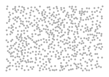
Figure 5.2. A ball process based on a Mattern hard core point process of type 2 (generated with Stochastic Geometry 4.1)

Based on a hard core PP, assign to each point of the PP a ball with a fixed radius (Figure 5.2). This model could be used to model a porous medium in 2D. However, in 3D we expect the grains of the porous medium matrix to touch some neighbors and that none of them is free without touching any neighbor. To achieve such a geometry, consider the following construction:

From a Voronoi-tessellation consider for each point $P_{c}$ of the PP the set of points $P_{b,i}$ where the corresponding Delaunay-diagram hits the grain boundaries. We may then interpolate these points by a smooth manifold to mark the surface of a grain. As an example, define

$$d(P_{c},x):=\sum_{i}\frac{(x-P_{c})^{2}}{(P_{b,,i}-P_{c})^{2}}\prod_{j\not=i}\frac{(x-P_{b,,j})^{2}}{(P_{b,i}-P_{b,,j})^{2}},\quad G(P_{c}):=\left\{x\in\mathbb{R}^{n}:d(P_{c},x)\leq 1\right\}$$

The sets $G(\cdot)$ could then model the grains of sand and the complement of the $G$ would be the porous medium.

6. Conclusion

We saw that asymptotic expansion can also be applied to stochastic geometries if they fulfill certain conditions, in particular stationarity and ergodicity. The method was applied to diffusion with and without nonlinear microscopic boundary conditions and to porous media flow. Some examples for stochastic geometries where given for solid and porous microstructures. Note that we did not treat homogenization of problems $\partial_{t}u^{\varepsilon}-\mbox{div}\,\left(\varepsilon^{2}D^{\varepsilon}\nabla u^{\varepsilon}\right)=f$ with $\varepsilon^{2}$-scaled diffusion. However, such problems can be treated even easier than the example calculation above with results of the form $\partial_{t}u_{0}-\mbox{div}_{\omega}\left(D\nabla_{\omega}u_{0}\right)=f$.

The results of this article can be considered as one more step towards understanding homogenization in non-periodic heterogeneous media. A big advantage of the presented approach is, that formal calculations require only few new theory. The only formal difference in the calculation is, that $\boldsymbol{Y}$ has to be changed into $\Omega$ and $y$ into $\omega$. Although the mathematical theory behind the rigorous calculations gets much more complex, the method’s user is not bothered by that. Indeed, besides some critical points in the calculations which were pointed out, one may not even think of the fact that one is doing stochastic calculations. The limit equations are independent on the particular realization which was used for homogenization. This is a feature of ergodicity and stationarity of the geometries.

A major issue for further investigations is the search for suitable models for geometries of natural heterogeneous media. Also, from the mathematical point of view, it would be nice to develop a “stochastic unfolding” corresponding to the periodic unfolding as a further theoretical foundation of the presented asymptotic expansion. Finally remark, that the intention of this paper was not to give a rigorous introduction to stochastic homogenization or the mathematics behind it but only to demonstrate that for non-mathematicians, switching from periodicity to stationary ergodic geometries can be easily achieved and would not bother the calculations or the results.

Appendix A Stochastic Geometries

This section follows [8] to introduce some basic mathematical concepts on random geometries. In particular, random closed sets and random measures will be defined rigorously. The connection to the periodic case was explained in detail in [8] and is based on similar ideas as the connections between periodic and stochastic asymptotic expansion. It will be shown that the assumptions on $A$, $B$ and $\Gamma$ in section 3.1 are reasonable and can be made w.l.o.g.. For more information on random closed sets, refer to Matheron [14] or Molchanov [17].

Let $\mathcal{F}(\mathbb{R}^{n})$ denote the set of all closed sets in $\mathbb{R}^{n}$. Then for $K\subset\mathbb{R}^{n}$ compact and $V\subset\mathbb{R}^{n}$ the following sets can be defined:

(A.1) $$\mathcal{F}_{V}:= \left\{F\in\mathcal{F}(\mathbb{R}^{n})\quad|\quad F\cap V\not=\emptyset\right\} V\subset\mathbb{R}^{n}\quad\textnormal{open set}$$

(A.2) $$\mathcal{F}^{K}:= \left\{F\in\mathcal{F}(\mathbb{R}^{n})\quad|\quad F\cap K=\emptyset\right\} K\subset\mathbb{R}^{n}\quad\textnormal{compact set}$$

The Fell topology on $\mathcal{F}(\mathbb{R}^{n})$ is created by the sets $\mathcal{F}_{V}$, $\mathcal{F}^{K}$ for all open V and compact K and according to [14], $(\mathcal{F}(\mathbb{R}^{n}),\mathcal{T}_{\mathcal{F}})$ is compact, Hausdorff and separable. The Matheron-$\sigma$-field $\sigma_{\mathcal{F}}$ is the Borel-$\sigma$-algebra created by the Fell-topology.

For a probability space $(\Omega,\sigma,\mu)$, a Random Closed Set (RACS) is a measurable mapping

$$\tilde{A}:(\Omega,\sigma,\mu)\longrightarrow(\mathcal{F},\sigma_{\mathcal{F}})\,.$$

It is the aim of this short introduction to demonstrate that such RACS have the nice properties which we assumed on $A$, $B$ and $\Gamma$ from section 3.1. Remark that up to now, a RACS is a mapping from a probability space into the set of closed subsets of $\mathbb{R}^{n}$.

In what follows, $\mathcal{M}(\mathbb{R}^{n})$ respectively $\mathcal{M}$ denotes the set of all locally finite Borel measures on $\mathbb{R}^{n}$. In Particular, $\mathcal{L}$ denotes the Lebesgue measure and $\mathcal{H}^{m}$ the $m$-dimensional Hausdorff measure. The smallest topology such that

$$\mathcal{M}\rightarrow\mathbb{R},\quad\tilde{\mu}\longmapsto\int f\,d\tilde{\mu}$$

is continuous for all $f\in C_{0}(\mathbb{R}^{n})$ is in general called the Vague-topology $\mathcal{T}_{\mathcal{V}}$ on $\mathcal{M}(\mathbb{R}^{n})$. The Borel-$\sigma$-field of this topology is denoted by $\sigma_{\mathcal{V}}$ respectively by $\mathcal{B}(\mathcal{M})$.

Theorem 1.

[6] $(\mathcal{M},\mathcal{T}_{\mathcal{V}})$ is a separable metric space. The $\sigma$-algebra $\sigma_{\mathcal{V}}$ on $\mathcal{M}$ created by the Vague topology $\mathcal{T}_{\mathcal{V}}$ is the smallest one, such that $\mu\mapsto\mu(B)$ is measurable for every bounded and measurable set $B\subset\mathbb{R}^{n}$.

A random measure on $\mathbb{R}^{n}$ is a measurable mapping $(\Omega,\sigma,\mu)\rightarrow(\mathcal{M},\sigma_{\mathcal{V}})$, $\omega\mapsto\mu_{\omega}$, where $(\Omega,\sigma,\mu)$ is a probability space. Random closed sets and the random measures are related due to the following Lemma, which implies that a random closed set always induces a random measure.

Lemma 2.

([24] Theorem 2.1.3 resp. Corollary 2.1.5)

Let $\mathcal{F}_{m}\subset\mathcal{F}$ be the space of closed m-dimensional sub manifolds of $\mathbb{R}^{n}$ such that the corresponding Hausdorff measure is locally finite. Then, the $\sigma$-algebra $\sigma_{\mathcal{F}}\cap\mathcal{F}_{m}$ is the smallest such that

$$M_{B}^{m}:\mathcal{F}_{m}\rightarrow\mathbb{R}\quad\Gamma\mapsto{\mathcal{H}}^{m}(\Gamma\cap B)$$

is measurable for every measurable and bounded $B\subset\mathbb{R}^{n}$.

It was part of the argumentation in [8] that due to Lemma 2 for any initial random closed manifold $A:(\Omega,\sigma,\mu)\rightarrow\mathcal{F}_{m}$ the assumptions $\Omega\subset\mathcal{M}$ and $\sigma=\mathcal{B}(\mathcal{M})\cap\Omega$ can be made w.l.o.g.. We introduced dynamical systems in section 3.1 and also defined ergodicity. However, one normally assumes only measurability of $\tau$ but the continuity is a rather direct consequence of $\Omega\subset\mathcal{M}$ [8].

A random measure is said to be stationary if for every $\omega\in\Omega$: $T(x)\mu_{\omega}=\mu_{\tau_{x}\omega}$ with

$$T(x)\mu_{\omega}(B):=\mu_{\omega}(B+x)\quad\forall B\in\mathcal{B}(\mathbb{R}^{n})$$

and a RACS $A$ is called stationary if $\chi_{A(\tau_{y}\omega)}(x)=\chi_{A(\omega)}(x+y)$ where $\chi_{A(\omega)}$ is the characteristic function of $A(\omega)$. This is slightly different introduction of stationarity than in section 3.1. However, we will see below that these definitions of stationarity and ergodicity already guaranty that RACS have the properties which we claimed in section 3.1. First, it is necessary to show that there is an equivalent of a Hausdorff-measure on $\Gamma$. This Hausdorff measure will be $\mu_{\Gamma,\mathcal{P}}$, stated by the following

Theorem 3.

(Mecke [15, 6]: Existence of Palm measure)

Let $\mathcal{L}$ be the Lebesgue-measure on $\mathbb{R}^{n}$ with $dx:=d\mathcal{L}(x)$ and $(\Omega,\sigma,\mu)$ as above. Then there exists a unique measure $\mu_{\mathcal{P}}$ on $\Omega$ such that

(A.3) $$\int_{\Omega}\int_{\mathbb{R}^{n}}f(x,\tau_{x}\omega)\,d\mu_{\omega}(x)d\mu(\omega)=\int_{\mathbb{R}^{n}}\int_{\Omega}f(x,\omega)\,d\mu_{\mathcal{P}}(\omega)dx$$

for all $\mathcal{B}(\mathbb{R}^{n})\times\mathcal{B}(\Omega)$-measurable non negative functions and all $\mu_{\mathcal{P}}\times\mathcal{L}$- integrable functions.

$\mu_{\mathcal{P}}$ as in Theorem 3 is called the Palm measure of $\mu_{\omega}$. Note that $\mu$ is the Palm measure of $\mathcal{L}$. For a random closed manifold $\Gamma:\,(\Omega,\sigma,\mu)\rightarrow\mathcal{F}_{m}\quad\omega\mapsto\Gamma(\omega)$ the random Hausdorff measure will be denoted by $\omega\mapsto\mu_{\Gamma(\omega)}$ and the Palm measure by $\mu_{\Gamma,\mathcal{P}}$.

Theorem 4.

(Ergodic Theorem [6])
Let the dynamical System $\tau_{x}$ be ergodic and assume that the stationary random measure $\mu_{\omega}$ has finite intensity. Then

(A.4) $$\lim_{t\rightarrow\infty}\frac{1}{t^{n}\mathcal{L}(A)}\int_{tA}g(\tau_{x}\omega)d\mu_{\omega}(x)=\int_{\Omega}g(\omega)d\mu_{\mathcal{P}}(\omega)$$

for $\mu$ almost surely in $\omega$ for all bounded Borel sets $A\supset\{|x|<1\}$ and all $g\in L^{1}(\Omega,\mu_{\mathcal{P}})$

For $\mu_{\Gamma(\omega)}^{\varepsilon}(B):=\varepsilon^{n}\mu_{\Gamma(\omega)}(\varepsilon^{-1}B)$ the latter theorem yields after a transformation of variables

(A.5) $$\lim_{\varepsilon\rightarrow 0}\int_{Q}f(x,\tau_{\frac{x}{\varepsilon}}\omega)d\mu_{\Gamma(\omega)}^{\varepsilon}=\int_{Q}\int_{\Omega}f(x,\omega)d\mu_{\Gamma,\mathcal{P}}dx\,.$$

for $f=\phi(x)\psi(\omega)$ with $\phi\in C_{0}^{\infty}(Q)$ and $\psi\in C_{b}(\Omega)$ and therefore also for $f\in C_{0}^{\infty}(Q;C_{b}(\Omega))$. This is a first indicator why we may consider $\mu_{\Gamma,\mathcal{P}}$ as a Hausdorff measure. It will be more striking by the following

Lemma 5.

[8] There is a measurable set, also denoted by $\Gamma\subset\Omega$, with $\chi_{\Gamma(\omega)}(x)=\chi_{\Gamma}(\tau_{x}\omega)$ for $\mathcal{L}+\mu_{\Gamma(\omega)}$-almost every $x$ for $\mu$-almost every $\omega$. Furthermore $\mu(\Gamma)=0$ and $\mu_{\Gamma,\mathcal{P}}(\Omega\backslash\Gamma)=0$.

The same proof also provides such a characteristic function for a $n$-dimensional random closed set $\tilde{A}$. $\tilde{\Gamma}:=\partial\tilde{A}$ is also a random closed set, which can be verified using $\mathcal{F}_{V}$ from (A.1) with $V=\tilde{A}\backslash\partial\tilde{A}$. In case $\tilde{\Gamma}$ is regular enough, there are subsets $A,\Gamma\subset\Omega$ such that $\chi_{\tilde{A}(\omega)}(x)=\chi_{A}(\tau_{x}\omega)$ and $\chi_{\tilde{\Gamma}(\omega)}(x)=\chi_{\Gamma}(\tau_{x}\omega)$. This is equally possible for $\tilde{B}:=\left(\mathbb{R}^{n}\backslash\tilde{A}\right)\cup\tilde{\Gamma}$. Thus, the assumptions made on $A$, $B$, and $\Gamma$ made in section 3.1 are now justified. Note that it is also possible to define $\nu_{\Gamma}:\Gamma\rightarrow\mathbb{R}^{n}$ such that $\nu_{\Gamma(\omega)}(x)=\nu_{\Gamma}(\tau_{x}\omega)$ and $\nu_{\Gamma}$ thus can be considered as normal field on $\Gamma$.

Note that in section 3.1, we started with $A,B,\Gamma\subset\Omega$ and defined $A(\omega)$, $B(\omega)$ and $\Gamma(\omega)$ to avoid these rather technical preliminaries. We conclude the mathematical part by some remarks on function spaces on $\Omega$ as well as on Gauss’ theorem and Poincaré inequalities.

Continuity and differentiability of functions were introduced in section 3.1. It is of course also possible to define arbitrarily high differentiability $C_{b}^{k}(\Omega)$. Since $\Omega$ is a separable metric space equipped with a measure $\mu$, it is possible to define

$$L^{p}(\Omega,\sigma,\mu):=\left\{f:\Omega\rightarrow\mathbb{R}\,:\,f\mbox{ is }\sigma-\mbox{measurable},\,\,\int\left|f\right|^{p}d\mu<\infty\right\}$$

These $L^{p}$-spaces have good properties, in particular they are separable and for any finite measure $\mu$ on $(\Omega,\mathcal{B}(\Omega))$ exists a countable dense set of $C_{b}^{\infty}(\Omega)$-functions in $L^{p}(\Omega,\mathcal{B}(\Omega),\mu)$ ($1\leq p<\infty$, $\mu$ $\sigma$-finite )[8].

It is of course possible to define various kinds of Sobolev spaces on $\Omega$. The reader is referred to [26, 27, 8].

Finally, in order to justify some of the calculations in section 4, it is vital to proof a Gauss-like theorem on stochastic spaces as well as some Poincaré inequalities.

Lemma 6.

[8] For all $\psi\in C_{b}^{1}(\Omega)$ and $\phi\in C_{b}^{1}(\Omega)^{n}$ holds:

(A.6) $$\int_{\Omega}\psi\nabla\phi d\mu=-\int_{\Omega}(\nabla\psi)\phi d\mu$$

Since the technique is very often used, we give the abbreviated proof from [8]:
Define $Q_{m}:=[-m,m]^{n}$. Then, since $\phi$ and $\psi$ are bounded, the Ergodic Theorem 4 leads to:

$$\int_{\Omega}\psi\nabla\phi d\mu = \lim_{m\rightarrow\infty}\frac{1}{(2m)^{n}}\int_{Q_{m}}\psi(\tau_{x}\omega)\nabla\phi(\tau_{x}\omega)dx$$

$$= \lim_{m\rightarrow\infty}\frac{1}{(2m)^{n}}\left(-\int_{Q_{m}}(\nabla\psi)(\tau_{x}\omega)\phi(\tau_{x}\omega)dx\right.$$

$$\phantom{\lim_{m\rightarrow\infty}\frac{1}{(2m)^{n}}\Big{(}}\left.+\int_{\partial Q_{m}}\nu_{Q_{m}}(x)(\phi\psi)(\tau_{x}\omega)d{\mathcal{H}}^{n-1}(x)\right)$$

$$= =\lim_{m\rightarrow\infty}\frac{1}{(2m)^{n}}\left(-\int_{Q_{m}}(\nabla\psi)(\tau_{x}\omega)\phi(\tau_{x}\omega)dx+\mathcal{O}(m^{n-1})\right)$$

$$= -\int_{\Omega}(\nabla\psi)\phi d\mu$$

where the integral over the boundary vanishes due to the fact that the surface of $Q_{m}$ grows with $(2m)^{n-1}$.QED

Note that (A.6) would also hold for an integral over $A$ if $\psi=0$ on $\Gamma$ or $\nabla\psi\cdot\nu_{\Gamma}=0$ on $\Gamma$ .

From the corresponding Poincaré inequalities on $\mathbb{R}^{n}$, one may conclude in the same way

$$\int_{\Omega}\left(\psi^{2}+\left|\nabla\psi\right|^{2}\right) \leq C\left(\int_{\Omega}\psi+\int_{\Omega}\left|\nabla\psi\right|^{2}\right)\quad\forall\psi\in C_{b}^{1}(\Omega)$$

$$\int_{A}\left(\psi^{2}+\left|\nabla\psi\right|^{2}\right) \leq C\int_{A}\left|\nabla\psi\right|^{2}\quad\forall\psi\in C_{b}^{1}(A)\mbox{ with }\psi=0\mbox{ on }\Gamma$$

where we have to assume that the constant $C$ for the realizations is independent on $\omega$:

$$\int_{Q_{m}\cap A(\omega)}\left(\psi^{2}(\tau_{x}\omega)+\left|\nabla\psi(\tau_{x}\omega)\right|^{2}\right)\leq C\int_{Q_{m}\cap A(\omega)}\left|\nabla\psi(\tau_{x}\omega)\right|^{2}+\mathcal{O}(m^{n-1})$$

Once such inequalities are established for $C_{b}^{1}$-functions, it is easy to expand them to corresponding Sobolev spaces on $\Omega$. (See [8, 9] for more complicated examples)

References

- [1] G. Allaire. Homogenization and two-scale convergence. SIAM Journal on Mathematical Analysis, 23:1482, 1992.
- [2] Grégoire Allaire. Homogenization of the navier-stokes equations with a slip boundary condition. Commun. Pure Appl. Math., 44(6):605–641, 1991.
- [3] Alain Bourgeat, Andro Mikelić, and Steve Wright. Stochastic two-scale convergence in the mean and applications. J. Reine Angew. Math., 456:19–51, 1994.
- [4] D. Cioranescu, A. Damlamian, and G. Griso. The periodic unfolding method in homogenization. SIAM J. Math. Anal., 40(4):1585–1620, 2008.
- [5] Doina Cioranescu, Alain Damlamian, and Georges Griso. Periodic unfolding and homogenization. C. R., Math., Acad. Sci. Paris, 335(1):99–104, 2002.
- [6] D.J. Daley and D. Vere-Jones. An Introduction to the Theory of Point Processes. Springer-Verlag New York, 1988.
- [7] Christof Eck. Homogenization of a phase field model for binary mixtures. Multiscale Model. Simul., 3(1):1–27, 2004.
- [8] Martin Heida. An extension of stochastic two-scale convergence and application. accepted by Asymptotic Analysis (In press), 2010.
- [9] Martin Heida. Stochastic homogenization or heat transfer in polycrystals with nonlinear contact conductivities. Submitted to Appl. Anal., 2011.
- [10] Ulrich (ed.) Hornung. Homogenization and porous media. Interdisciplinary Applied Mathematics. 6. New York, NY: Springer. xvi, 275 p., 1997.
- [11] Hans-Karl Hummel. Homogenization for heat transfer in polycrystals with interfacial resistances. Appl. Anal., 75(3-4):403–424, 2000.
- [12] D. Lukkassen and P. Wall. Two-scale convergence with respect to measures and homogenization of monotone operators. J. Funct. Spaces Appl, 3(2):125–161, 2005.
- [13] Anna Marciniak-Czochra and Mariya Ptashnyk. Derivation of a macroscopic receptor-based model using homogenization techniques. SIAM J. Math. Anal., 40(1):215–237, 2008.
- [14] G. Matheron. Random sets and integral geometry. 1975.
- [15] J. Mecke. Stationäre zufällige Maße auf lokalkompakten abelschen Gruppen. Probability Theory and Related Fields, 9(1):36–58, 1967.
- [16] C. Miehe and C. G. Bayreuther. On multiscale fe analyses of heterogeneous structures: from homogenization to multigrid solvers. International Journal for Numerical Methods in Engineering, 71(10):1135–1180, 2007.
- [17] Ilya Molchanov. Theory of random sets. Probability and Its Applications. London: Springer. xvi, 488 p., 2005.
- [18] M. Neuss-Radu. Some extensions of two-scale convergence. Comptes rendus de l’Académie des sciences. Série 1, Mathématique, 322(9):899–904, 1996.
- [19] M. Neuss-Radu. The boundary behavior of a composite material. Mathematical Modelling and Numerical Analysis, 35(3):407–435, 2001.
- [20] M. Neuss-Radu and W. Jäger. Effective transmission conditions for reaction-diffusion processes in domains separated by an interface. SIAM Journal on Mathematical Analysis, 39(3):687–720, 2008.
- [21] G. Nguetseng. A general convergence result for a functional related to the theory of homogenization. SIAM Journal on Mathematical Analysis, 20:608, 1989.
- [22] Malte A. Peter. Coupled reaction-diffusion processes inducing an evolution of the microstructure: Analysis and homogenization. Nonlinear Analysis, 70:806–821, 2009.
- [23] Dietrich Stoyan, Wilfrid S. Kendall, and Joseph Mecke. Stochastic geometry and its applications. Reprint of the 1995 2nd hardback ed. Hoboken, NJ: John Wiley & Sons. xix, 436 p., 2008.
- [24] M. Zaehle. Random processes of hausdorff rectifiable closed sets. Math. Nachr., 108:49–72, 1982.
- [25] V.V. Zhikov. On an extension of the method of two-scale convergence and its applications. Sbornik: Mathematics, 191(7):973–1014, 2000.
- [26] V.V. Zhikov, S.M. Kozlov, and O.A. Olejnik. Homogenization of differential operators and integral functionals. Transl. from the Russian by G. A. Yosifian. Berlin: Springer-Verlag. xi, 570 p., 1994.
- [27] V.V. Zhikov and A.L. Pyatniskii. Homogenization of random singular structures and random measures. Izv. Math., 70(1):19–67, 2006.