G.Y. Chen¹ and J.P. Ma^2,3

¹ Department of Physics, Peking University, Beijing 100871, China

² Institute of Theoretical Physics, Academia Sinica, Beijing 100190, China

³ Center for High-Energy Physics, Peking University, Beijing 100871, China

Abstract

We have proposed to use an effective theory to describe interactions of an $N\bar{N}$-system. The effective theory can be constructed in analogy to the existing effective theory for an $NN$-system. In this work we study the next-to-leading order correction to $N\bar{N}$ scattering near the threshold in the effective theory. We find that the experimental data can be well described with the effective theory.

Interactions between a nucleon and an antinucleon have been studied extensively with potential models(see [1, 2, 3] and references therein). In general the potential of these models includes various effects of meson exchanges and is supplemented with a phenomenologically determined imaginary part to account for the $N\bar{N}$ annihilation. The descriptions of the low energy $N\bar{N}$ scattering with these potential models are successful. Recently there is a renewed interest to study $N\bar{N}$ interactions, stimulated by experimental observations of the threshold enhancement of a $p\bar{p}$ system in the radiative decay of $J/\psi$[4], $B$-decays[5] and $e^{+}e^{-}$-annihilations[6]. It has been shown that the enhancement can be explained with the final state interaction, where the enhancement is determined by the $N\bar{N}$ scattering amplitude near the threshold [7, 8, 9, 11, 12, 13, 14, 15, 16, 17].

Because the momentum transfer in $N\bar{N}$ scattering near the threshold is small, the inner structure of a nucleon or antinucleon can not be seen. This indicates that one can take the nucleon and antinucleon as point-like particles and construct an effective theory to describe the $N\bar{N}$ scattering near the threshold. Near the threshold the interactions through $\pi$-exchanges are most important among those of exchanges of other mesons. hence, the effective theory only contains $N$-, $\bar{N}$- and $\pi$-fields. In [17] we have proposed such an effective theory. We have used the tree-level result of the effective theory and a partial sum of higher order effects to successfully describe the observed enhancement and the $N\bar{N}$ scattering near the threshold. In this work we study the next-to-leading order correction in the effective theory.

An effective theory for an $N\bar{N}$ system near the threshold can be constructed in analogy to the effective theory for an $NN$ system. The effective theory for the $NN$ system has been proposed in[18, 19, 20] and studied extensively in [19, 20, 21]. In constructing such an effective theory one makes an power expansion in the momentum near the threshold. In the effective theory, the U.V. divergences are regularized with the dimensional regularization. The interactions with $\pi$-mesons are fixed with chiral symmetry. A power counting to determine the relative importance of different terms in the effective theory has to be established. But, there are distinct difference between the effective theory of $N\bar{N}$ interactions and that of $NN$ interactions.

It is well-known that for an $NN$ system the scattering lengthes are large and there is a shallow bound state in ${}^{3}S_{1}-{{}^{3}}D_{1}$ channel and a virtual state in ${}^{1}S_{0}$ channel. To take these facts into account in the effective theory, the power subtraction scheme has been introduced[20]. With this scheme a systematic power counting of the effective theory can be established. In the case of $N\bar{N}$ systems, the scattering lengthes, according LEAR experiment[7] and model results[8], are around 1fm. They are much smaller than those of $NN$ systems. Therefor one can use the minimal subtraction scheme and hence the simple power counting for the effective theory of $N\bar{N}$ systems.

Another difference is that an $N\bar{N}$ system can be annihilated into mesons, while a $NN$ system can not be annihilated. The annihilation of an $N\bar{N}$ system into virtual or real mesons results in that the dispersive and absorptive part of the $N\bar{N}$ scattering amplitudes are relatively of the same importance. In order to incorporate this fact some coupling constants in the effective theory of an $N\bar{N}$ system are complex numbers. One should keep in mind that the complex coupling constants here do not mean the violation of time-reversal symmetry. The effective Lagrangian with complex coupling constants should be understood as for the purpose to effectively build the $S$-operator and hence scattering amplitudes. This can be understood as the following: One can imagine that the effective theory is obtained from a perturbative matching of a more fundamental theory. In the more fundamental theory with the time-reversal symmetry scattering amplitudes can become complex beyond tree-level because absorptive parts can exist at one- or more loop level. The imaginary parts of the coupling constants in the effective theory are from these absorptive parts in the matching. If the underlying theory respects to the time-reversal symmetry and other discrete symmetry like charge-conjugation and parity, the generated operators through the matching in the effective theory can not violate these discrete symmetries of the underlying theory. This fact also tell us that the effective theory should be built with these operators which are $C$-, $P$- and $T$-even.

At low energy, i.e., for an $N\bar{N}$ system near its threshold, we need to consider theory contains contact interactions and interactions with pions which is consistent with chiral symmetry. At low energy we can use the nonrelativistic fields to describe the nucleon $N$. The nonrelativistic fields are given as

$$\psi=\left(\begin{array}[]{c}\psi_{p}\\ \psi_{n}\\ \end{array}\right),\ \ \ \ \ \ \chi=\left(\begin{array}[]{c}\chi_{p}\\ \chi_{n}\\ \end{array}\right).$$ (1)

The field $\psi(\chi^{\dagger})$ annihilates a nucleon(an antinucleon) and the field $\psi^{\dagger}(\chi)$ creates a nucleon(an antinucleon). The pion-field is defined with Pauli matrices $\tau^{i}$ acting in the isospin space as:

$$\xi(x)=e^{i\frac{M}{2f_{\pi}}},\ \ \ \ M=\tau^{i}\pi^{i}=\left(\begin{array}[]{cc}\pi^{3}&\pi^{1}-i\pi^{2}\\ \pi^{1}+i\pi^{2}&-\pi^{3}\\ \end{array}\right),$$ (2)

with $f_{\pi}\approx 93$ MeV. The field $\pi^{i}(i=1,2,3)$ is real. Under $SU(2)_{L}\times SU(2)_{R}$ chiral symmetry the fields transform as

$$\xi\rightarrow L\xi U^{\dagger}=U\xi R^{\dagger},\ \ \Sigma\equiv\xi^{2}\rightarrow L\Sigma R^{\dagger},\ \ \psi\rightarrow U\psi,$$ (3)

where L, R are global transformations in $SU(2)_{L}$ and $SU(2)_{R}$ respectively and $U$ is a pion-field-dependent SU(2) matrix. From $\xi$ we can give out the vector and axial-vector pion currents as

$$V_{\mu}=\frac{1}{2}(\xi\partial_{\mu}\xi^{\dagger}+\xi^{\dagger}\partial_{\mu}\xi),\ \ \ A_{\mu}=\frac{i}{2}(\xi\partial_{\mu}\xi^{\dagger}-\xi^{\dagger}\partial_{\mu}\xi),$$ (4)

where the axial current $A_{\mu}$ and the chiral covariant derivative $D_{\mu}=(\partial_{\mu}+V_{\mu})$ transform linearly as

$$A_{\mu}\rightarrow UA_{\mu}U^{\dagger},\ \ \ D_{\mu}\rightarrow UD_{\mu}U^{\dagger}.$$ (5)

With the above fields the effective Lagrangian can be constructed as:

$$\mathcal{L}_{eff} = \mathcal{L}_{N}+\mathcal{L}_{\pi},$$

$$\mathcal{L}_{N} = \psi^{\dagger}(iD_{0}+{\bf{D}}^{2}/2m)\psi+\chi^{\dagger}(iD_{0}-{\bf{D}}^{2}/2m)\chi+\frac{c_{0}}{4}\psi^{\dagger}\chi\chi^{\dagger}\psi+\frac{c_{1}}{4}\psi^{\dagger}\tau^{i}\chi\chi^{\dagger}\tau^{i}\psi$$

$$+\frac{d_{0}}{4}\psi^{\dagger}\sigma^{i}\chi\chi^{\dagger}\sigma^{i}\psi+\frac{d_{1}}{4}\psi^{\dagger}\tau^{i}\sigma^{j}\chi\chi^{\dagger}\sigma^{j}\tau^{i}\psi+g_{A}\psi^{\dagger}\mbox{\boldmath{$\sigma$}}\cdot{\bf{A}}\psi+g_{A}\chi^{\dagger}\mbox{\boldmath{$\sigma$}}\cdot{\bf{A}}\chi+\mathcal{O}(p^{2}),$$

$$\mathcal{L}_{\pi} = \frac{f_{\pi}^{2}}{4}\mbox{Tr}\partial_{\mu}\Sigma^{\dagger}\partial^{\mu}\Sigma+\frac{m_{\pi}^{2}f_{\pi}^{2}}{4}\mbox{Tr}(\Sigma+\Sigma^{\dagger})+\mathcal{O}(p^{4}),$$ (6)

where $g_{A}\approx 1.25$. $c_{I}$ with the isospin index $I$ is the coupling constant in the ${}^{1}S_{0}$ channel, while $d_{I}$ is the coupling constant in the ${}^{3}S_{1}$ channel. These coupling constants are in general complex to account for the $N\bar{N}$ annihilation.

The power counting of the effective theory is discussed in detail in[17]. It is easy from the effective Lagrangian to derive the tree-level $N\bar{N}$ scattering amplitude. The amplitude is an expansion in the three momentum $p$ of $N$ or $\bar{N}$. The leading order is at order of $p^{0}$. the amplitude at this order is determined by those contact terms given explicitly in Eq.(6) and the interaction from exchange of single $\pi$. We will consider the momentum region $p\sim m_{\pi}$. From Eq.(6), the $NN\pi$- or $\bar{N}\bar{N}\pi$ vertex is proportional to $p$. In the single $\pi$-exchange, the power of $p$ from the two vertices is canceled by the power of the denominator of the $\pi$-propagator. This is why the amplitude with single $\pi$-exchange is taken at order of $p^{0}$. The next-to-leading order is at order of $p$ and is determined by one-loop diagrams. It should be noted that some of one-loop diagrams will not contribute at the order. They can contribute at order of $p^{2}$ or higher. As we will show that it is easy to find those one-loop diagrams which give the contributions at order of $p$. At order of $p^{2}$ the amplitude receives corrections from different sources. The corrections can come from those one-loop diagrams which contribute at order of $p^{2}$ and come from two-loop diagrams. They also come from those contact terms in the effective Lagrangian at order of $p^{2}$, which we have not included in Eq.(6). Those contact terms in general contain derivatives. We will use the dimensional regularization and the minimal subtraction scheme as discussed before.

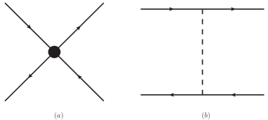
Figure 1: The leading order diagrams. Fig.1a is for the contact terms, Fig.1b is from one $\pi$-exchange.

After giving the effective theory, we now consider the $N\bar{N}$ scattering near the threshold:

$$N(\vec{p},s_{1})+\bar{N}(-\vec{p},s_{2})\rightarrow N(\vec{k},s_{1}^{\prime})+\bar{N}(-\vec{k},s_{2}^{\prime}),\ \ \ |\vec{p}|=p=\beta\sqrt{m^{2}+p^{2}},$$ (7)

where $\vec{p}$ and $\vec{k}$ are three-momentum. The spins are denoted as $s^{,}$s. $\beta$ is the velocity. $m$ is the mass of nucleons. As discussed before, the leading order contribution is at $\mathcal{O}(p^{0})$. The contributions at this order can be represented by diagrams in Fig.1. The leading order amplitude can be expressed as,

$$\mathcal{T}^{(0)} = \frac{c_{0}}{4}\xi^{\dagger}\eta\eta^{\dagger}\xi+\frac{c_{1}}{4}\xi^{\dagger}\tau^{a}\eta\eta^{\dagger}\tau^{a}\xi+\frac{d_{0}}{4}\xi^{\dagger}\sigma^{i}\eta\eta^{\dagger}\sigma^{i}\xi+\frac{d_{1}}{4}\xi^{\dagger}\sigma^{i}\tau^{a}\eta\eta^{\dagger}\sigma^{i}\tau^{a}\xi$$ (8)

$$+(\frac{g_{A}}{2f_{\pi}})^{2}\xi^{\dagger}\vec{\sigma}\cdot(\vec{p}-\vec{k})\tau^{a}\xi\eta^{\dagger}\vec{\sigma}\cdot(\vec{p}-\vec{k})\tau^{a}\eta\frac{1}{(p-k)^{2}-m_{\pi}^{2}},$$

where $\xi$ and $\eta$ are the spinors of the nucleon and antinucleon respectively.

At one-loop level, not all diagrams give contributions at the order $\mathcal{O}(p^{1})$. At one-loop level one meets a loop integral of a four momentum $k$. One can perform the $k^{0}$-integration first by using a contour in the complex $k^{0}$-plan. The contribution of the integration comes from poles insider the contour. The poles can appear from denominators of nucleon propagators or $\pi$-propagators. It is easy to show that only those contributions from the poles of nucleon propagators are at the order $\mathcal{O}(p^{1})$, while other contributions are at higher orders. With this in mind, only those diagrams at one-loop given in Fig.2 give contributions at the next-to-leading order.

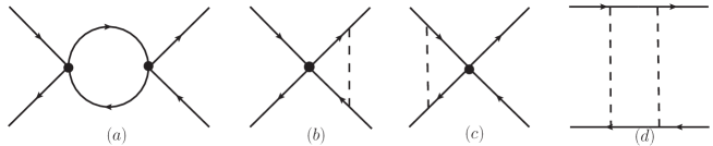
Figure 2: The diagrams which give the next-to-leading order corrections.

It is rather straightforward to evaluate these loop contributions. In fact results of some loop integrals exist in the literature. Hence, we give here the results without showing here detailed calculations. It should be noted that all contributions in Fig.2 are finite in the dimensional regularization. As discussed in the above, we will use the minimal subtraction scheme for renormalization. In this case, the next-to-leading order contributions do not depend on the renormalization scale $\mu$, or the subtraction point. The $\mu$-dependence of coupling constants starts at order of $p^{2}$. The contributions from Fig.2a read:

$$\mathcal{T}\biggr{|}_{2a}=i\frac{mk}{4\pi}\left[\frac{c_{0}^{2}}{4}\xi^{\dagger}\eta\eta^{\dagger}\xi+\frac{c_{1}^{2}}{4}\xi^{\dagger}\tau^{a}\eta\eta^{\dagger}\tau^{a}\xi+\frac{d_{0}^{2}}{4}\xi^{\dagger}\sigma^{i}\eta\eta^{\dagger}\sigma^{i}\xi+\frac{d_{1}^{2}}{4}\xi^{\dagger}\sigma^{i}\tau^{a}\eta\eta^{\dagger}\sigma^{i}\tau^{a}\xi\right],$$ (9)

we note that this contribution with the minimal subtraction scheme can be equivalently calculated by taking a cut cutting the nucleon loop in Fig.2a.

The contributions from Fig.2b and Fig.2c read:

$$\mathcal{T}\biggr{|}_{2b} = -i\frac{1}{4\pi}(\frac{g_{A}}{2f_{\pi}})^{2}\eta^{\dagger}\Gamma^{(c)}\xi\cdot\left[I_{0}(k)\xi^{\dagger}\sigma^{i}\tau^{a}\Gamma^{(c)}\sigma^{i}\tau^{a}\eta+I_{1}(k)\xi^{\dagger}\vec{\sigma}\cdot\vec{k}\tau^{a}\Gamma^{(c)}\vec{\sigma}\cdot\vec{k}\tau^{a}\eta\right],$$

$$\mathcal{T}\biggr{|}_{2c} = -i\frac{1}{4\pi}(\frac{g_{A}}{2f_{\pi}})^{2}\xi^{\dagger}\Gamma^{(c)}\eta\cdot\left[I_{0}(k)\eta^{\dagger}\sigma^{i}\tau^{a}\Gamma^{(c)}\sigma^{i}\tau^{a}\xi+I_{1}(k)\eta^{\dagger}\vec{\sigma}\cdot\vec{p}\tau^{a}\Gamma^{(c)}\vec{\sigma}\cdot\vec{p}\tau^{a}\xi\right].$$ (10)

In the above $\Gamma^{(c)}$ is a matrix acting in the spin- and isospin space. The sum of the direct product $\Gamma^{(c)}\otimes\Gamma^{(c)}$ is implied. The sum reads:

$$\Gamma^{(c)}\otimes\Gamma^{(c)}=\frac{c_{0}}{4}I\otimes I+\frac{c_{1}}{4}\tau^{a}\otimes\tau^{a}+\frac{d_{0}}{4}\sigma^{i}\otimes\sigma^{i}+\frac{d_{1}}{4}\sigma^{i}\tau^{a}\otimes\sigma^{i}\tau^{a}.$$ (11)

The functions $I_{0}$ and $I_{1}$ are from loop-integrals. They are:

$$I_{0}(k) = \frac{mk}{4}\left[1+y-iy\sqrt{2y}+y(y+2)\left(-\frac{1}{2}\ln(1+\frac{2}{y})+i\tan^{-1}\sqrt{\frac{2}{y}}\right)\right],$$

$$I_{1}(k) = \frac{m}{4k}\left[1-3y+3iy\sqrt{2y}-y(2+3y)\left(-\frac{1}{2}\ln(1+\frac{2}{y})+i\tan^{-1}\sqrt{\frac{2}{y}}\right)\right].$$ (12)

$$y=\frac{m_{\pi}^{2}}{2\vec{k}^{2}},\ \ k=\sqrt{\vec{k}^{2}}.$$

The contributions from Fig.2d are the most difficult parts. However, the relevant results of loop integrals can be found in [22]. We have numerically checked these results and found an agreement. The contributions can be written in the form:

$$\mathcal{T}\biggr{|}_{2d} = m(\frac{g_{A}}{2f_{\pi}})^{4}\biggr{\{}F_{S}\left(3\xi^{\dagger}\xi\eta^{\dagger}\eta+2\xi^{\dagger}\tau^{a}\xi\eta^{\dagger}\tau^{a}\eta\right)-\left(3\xi^{\dagger}\sigma^{i}\xi\eta^{\dagger}\sigma^{j}\eta+2\xi^{\dagger}\sigma^{i}\tau^{a}\xi\eta^{\dagger}\sigma^{j}\tau^{a}\eta\right)$$ (13)

$$\cdot\left(F_{V}\delta^{ij}+F_{W}(k-p)^{i}(k-p)^{j}+F_{T}(\vec{k}\times\vec{p})^{i}(\vec{k}\times\vec{p})^{j}\right)$$

$$+iF_{P}(\vec{k}\times\vec{p})^{i}\left(3\xi^{\dagger}\sigma^{i}\xi\eta^{\dagger}\eta-3\xi^{\dagger}\xi\eta^{\dagger}\sigma^{i}\eta+2\xi^{\dagger}\sigma^{i}\tau^{a}\xi\eta^{\dagger}\tau^{a}\eta-2\xi^{\dagger}\tau^{a}\xi\eta^{\dagger}\tau^{a}\sigma^{i}\eta\right)\biggr{\}},$$

the functions $F_{S,V,T,W,P}$ are given as:

$$F_{S} = -\frac{1}{16\pi}\left\{4(2m_{\pi}^{2}+q^{2})\Gamma_{0}(p)+2q^{2}\Gamma_{1}(p)-4ip-(2m_{\pi}^{2}+q^{2})^{2}G_{0}(p,q)\right\},$$

$$F_{W} = -\frac{1}{q^{2}}F_{V}=\frac{1}{4\pi}G_{2}(p,q),$$

$$F_{P} = \frac{1}{8\pi}\left\{2\Gamma_{0}(p)+2\Gamma_{1}(p)-(2m_{\pi}^{2}+q^{2})\left[G_{0}(p,q)+2G_{1}(p,q)\right]\right\},$$

$$F_{T} = -\frac{1}{4\pi}\left\{G_{0}(p,q)+4G_{1}(p,q)+4G_{3}(p,q)\right\},$$ (14)

where the complex-valued functions are given as,

$$\Gamma_{0}(p) = \frac{1}{2p}\left[\arctan\frac{2p}{m_{\pi}}+i\ln\frac{u}{m_{\pi}}\right],\ \ \ \ \ \ \ u=\sqrt{m_{\pi}^{2}+4p^{2}},$$

$$\Gamma_{1}(p) = \frac{1}{2p^{2}}\left[m_{\pi}+ip-(m_{\pi}^{2}+2p^{2})\Gamma_{0}(p)\right],$$

$$G_{0}(p,q) = \frac{1}{qR}\left[\arcsin\frac{qm_{\pi}}{uw}+i\ln\frac{pq+R}{um_{\pi}}\right],\ \ \ R=\sqrt{m_{\pi}^{4}+p^{2}w^{2}},\ \ \ w=\sqrt{4m_{\pi}^{2}+q^{2}},$$

$$G_{1}(p,q) = \frac{\Gamma_{0}(p)-2A(q)-(m_{\pi}^{2}+2p^{2})G_{0}(p,q)}{4p^{2}-q^{2}},\ \ \ \ A(q)=\frac{1}{2q}\arctan\frac{q}{2m_{\pi}},$$

$$G_{2}(p,q) = p^{2}G_{0}(p,q)+(m_{\pi}^{2}+2p^{2})G_{1}(p,q)+A(q),$$

$$G_{3}(p,q) = \frac{\frac{1}{2}\Gamma_{1}(p)-p^{2}G_{0}(p,q)-2(m_{\pi}^{2}+2p^{2})G_{1}(p,q)}{4p^{2}-q^{2}}.$$ (15)

where we define $q=|\vec{k}-\vec{p}|$ here. The total results can be written as:

$$\mathcal{T}(\vec{p},\vec{k})=\mathcal{T}^{(0)}(\vec{p},\vec{k})+\mathcal{T}^{(1)}(\vec{p},\vec{k})+\mathcal{O}(p^{2}),$$ (16)

where $\mathcal{T}^{(0)}$ is given in Eq.(8) and the order $\mathcal{O}(p^{1})$ result is:

$$\mathcal{T}^{(1)}=\mathcal{T}\biggr{|}_{2a}+\mathcal{T}\biggr{|}_{2b}+\mathcal{T}\biggr{|}_{2c}+\mathcal{T}\biggr{|}_{2d}$$ (17)

With the above results we have the complete result for $N\bar{N}$ scattering near the threshold at the next-to-leading order. We will use this result to fit the experimental data.

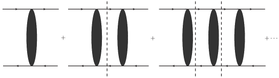
Figure 3: The narrow and long bubble represents the amplitude $\mathcal{A}_{[j\ell\ell^{\prime}s,I]}(E)$ at certain order with the subtraction of contributions from physical cuts or cut diagrams. The sum of diagrams can be performed.

Our results for the scattering amplitude can be further improved by including some higher order corrections without a concrete calculation. We have noticed in [16, 17] that some corrections from higher orders can be summed into a compact form. The summation can be done for partial waves. We define our partial waves from the $N\bar{N}$ scattering amplitude $\mathcal{T}_{I}(\vec{p},\vec{k},s_{1},s_{2},s_{1}^{\prime},s_{2}^{\prime})$ with the isospin $I=0,1$ as:

$$\mathcal{T}_{I}(\vec{p},\vec{k},s_{1},s_{2},s_{1}^{\prime},s_{2}^{\prime}) = \sum Y^{\ast}_{\ell\ell_{3}}(\vec{p}/p)Y_{\ell^{\prime}\ell_{3}^{\prime}}(\vec{k}/k)(1/2,s_{1};1/2,s_{2}|s,s_{3})(1/2,s_{1}^{\prime};1/2,s_{2}^{\prime}|s^{\prime},s_{3}^{\prime})$$ (18)

$$\cdot(\ell,\ell_{3},s,s_{3}|j,j_{3})(\ell^{\prime},\ell_{3}^{\prime},s^{\prime},s_{3}^{\prime}|j^{\prime},j_{3}^{\prime})\delta_{jj^{\prime}}\delta_{j_{3}j_{3}^{\prime}}\delta_{ss^{\prime}}\mathcal{T}_{[j\ell\ell^{\prime}s,I]}(E).$$

In the above the repeated indexes are summed and $E$ is the total kinetic energy $E=p^{2}/m$ of the system. The summation can be explained with Fig.3. We will take $s$-waves as examples to illustrate this.

Supposing we have calculated the scattering amplitude $\mathcal{T}_{[0000,0]}(E)$ at certain orders and we denote this amplitude as $\mathcal{A}_{[0000,0]}(E)$, in which possible contributions from physical cuts or cut diagrams are subtracted. At tree-level, $\mathcal{A}_{[0000,0]}(E)$ is just the tree-level amplitude. At the next-to-leading order $\mathcal{A}_{[0000,0]}(E)$ is determined by diagrams from Fig.1 and those from Fig.2 after subtracting the contributions of cut diagrams of Fig.2. In Fig.3 we denote this amplitude with the narrow long bubble. Now using this amplitude $\mathcal{A}_{[0000,0]}(E)$ one can generate those diagrams as ladder diagrams at higher orders as shown in Fig.3. Physically the interpretation of Fig.3 is the following: The $N\bar{N}$ undergoes a multiple scattering process $N\bar{N}\to N\bar{N}\to\cdots\to N\bar{N}$. Each scattering is due to the amplitude $\mathcal{A}_{[0000,0]}(E)$ Each pair of $N\bar{N}$ is on-shell in Fig.3. We will call amplitudes for such a multiple scattering process as rescattering amplitudes. It is easy to shown that the sum of these diagrams is the sum of a geometric series. One then finds the sum for the amplitude as:

$${\mathcal{T}}_{[0000,0]}(E)={\mathcal{A}}_{[0000,0]}(E)\left[1-i\frac{m^{2}\beta}{(4\pi)^{2}}{\mathcal{A}}_{[0000,0]}(E)\right]^{-1}+\cdots.$$ (19)

This can be generalized to other partial waves. We will improve our result by adding the rescattering effects. The improvement is done only for $S$-waves with the assumption that the amplitudes with small $\ell$ are dominant because of the finite interaction range. A small complication is with the case of $s=1$ is that there is a mixing of $S$-waves and $D$-waves. In this case, the summation takes a form of $2\times 2$ matrix. Details can be found in [17].

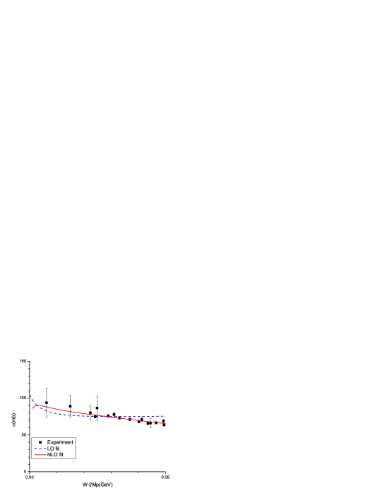
Figure 4: The fitting results for the cross-section of $p\bar{p}$ elastic scattering. The dashed line is the leading order fit. The solid line is the next-to-leading order fit.

We have performed numerical fits with our results for experimental data. The data are taken from [23]. In [17] we have studied the $p\bar{p}$ scattering and the enhancement in $J/\psi\to\gamma p\bar{p}$ and $e^{+}e^{-}\to p\bar{p}$ together with a combined fit. For the enhancement, certain assumptions have been made in [17] to relate the observed enhancement to $N\bar{N}$ scattering near the threshold. In fact, the study of the enhancement can also be done with the approach of effective theories in a consistent way combined with the effective theory here for $N\bar{N}$ system. We leave this to future works. Here we only focus on $p\bar{p}$ elastic scattering in order to see how good our effective theory works. In Fig.4. we give our fitting result with the amplitude at leading and next-to-leading order, respectively. With our results we are able to describe the experimental data below $E\sim 50$MeV, corresponding to $p\sim 200$MeV. The fitting quality with the leading and the next-to-leading result is given by $\chi/d.o.f.\approx 2.6$ and $\chi/d.o.f.\approx 1.7$, respectively. At tree-level we can not determine the coupling $c_{0,1}$ or $d_{0,1}$ separately, because they appear as the combination as $c_{0}+c_{1}$ or $d_{0}+d_{1}$ in the amplitude. With the NLO results we can determine these coupling constants in the unit of ${\rm GeV}^{-2}$ as:

$$c_{0}=(180\pm 4)+i(20\pm 3),\ \ \ c_{1}=-211+i87,\ \ \$$

$$d_{0}=-(60\pm 2)+i(61\pm 4),\ \ \ d_{1}=(37\pm 3)+i(56\pm 4).$$ (20)

where the fitting errors are given in the brackets. For $c_{1}$ the errors are very small in comparison with the numbers. We hence do not give the errors. From Fig.4. one can see that our NLO amplitude can describe experimental data well. With the determined couplings we can also determine the scattering lengthes of $S$-waves:

$$a_{[^{1}S_{0},0]}=-(5.88\pm 0.22)-i(1.12\pm 0.17),\ \ a_{[^{1}S_{0},1]}=0.67-i0.09,\ \$$

$$a_{[^{3}S_{1},0]}=4.24-i0.06,\ \ a_{[^{3}S_{1},1]}=-(0.25\pm 0.06)-i(1.08\pm 0.08),$$ (21)

in unit of ${\rm fm}$. In the above the last integer in $[\cdots]$ indicates the isospin $I=0$ or $I=1$.

We have also performed the numerical fits by adding the rescattering effects into the leading- and next-to-leading amplitude as discussed in the above. The fitting results are represented in Fig.5. From Fig.5. one can realize that with the rescattering effects the experimental data can also be well described, indicated by $\chi/d.o.f.\approx 1.7$. From the fit with next-to-leading amplitude and rescattering effects we have for the coupling constants in unit of ${\rm GeV}^{-2}$ as:

$$c_{0}=(70\pm 37)+i(0\pm 190),\ \ \ c_{1}=(132\pm 92)+i(0\pm 248),$$

$$d_{0}=-(25\pm 2)+i(0\pm 14),\ \ \ d_{1}=-(38\pm 8)+i(99\pm 80).$$ (22)

The corresponding scattering lengthes are

$$a_{[^{1}S_{0},0]}=(0.3\pm 2)-i(0\pm 10),\ \ a_{[^{1}S_{0},1]}=(0.34\pm 0.09)-i(0.00\pm 0.24),\ \$$

$$a_{[^{3}S_{1},0]}=4.21-i(0\pm 0.01),\ \ a_{[^{3}S_{1},1]}=(1.20\pm 0.15)-i(1.91\pm 1.54).$$ (23)

The determined scattering lengthes are qualitatively in agreement with results from some models[8] and from LEAR experiment[7]. They are smaller or much smaller than those of an $NN$ system. This fact supports the argument for using the minimal subtraction scheme and hence the standard power counting for our effective theory.

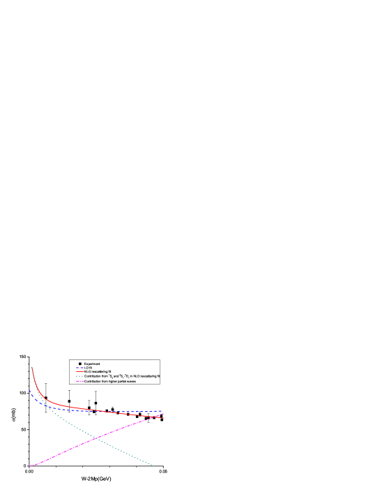
Figure 5: The fitting result for the cross-section of $p\bar{p}$ elastic scattering. The dashed line is the leading order fit. The solid line is the next to leading order fit while including the rescattering effect in ${}^{1}S_{0}$ and ${}^{3}S_{1}-{{}^{3}}D_{1}$ channel. The dotted line is the contribution from ${}^{1}S_{0}$ and ${}^{3}S_{1}-{{}^{3}D_{1}}$ with the rescattering amplitude. The dashed-dotted line is the contribution from all the other partial waves up to the next-to-leading order.

Although the data can be well described from Fig.5, the significant changes in some coupling constants indicate that corrections from higher orders can be significant. In Fig.5 we also give results for the contributions from those partial waves with $\ell\neq 0$ where the contribution from the partial wave ${}^{3}D_{1}$ is subtracted. These contributions essentially come from $\pi$-exchanges. From Fig.5. we can see that these contributions will become dominant when the total energy $E$ is approaching to the value around $50$MeV, corresponding to $p\sim 200$MeV. This indicates that the expansion in $p$ of the effective theory converges slowly or applicable region of the effective theory is small. This has also been found in the effective theory of an $NN$ system. The study in [21] shows that the contributions from $\pi$-exchanges become dominant and much larger than predictions at leading orders around $p\sim 100$MeV in some spin triplet channels. The reason for this is the true expansion parameter for $\pi$-exchanges is at order of $(g_{A}^{2}m_{\pi}m)/(8\pi f^{2}_{\pi})$. Because the nucleon mass $m$ is large in comparison with $f_{\pi}$, the expansion parameter is not small. In our case in which contributions from $\pi$-exchanges become dominant at $p\sim 100$MeV, the situation seems better than that for $NN$ systems, because the coupling constants of the local interactions, which give the important contributions at leading order, are roughly twice larger than the corresponding coupling constants in the effective theory of an $NN$-system.

It is interesting to compare the approach of the effective theory with the approach of the the effective range expansion for describing $N\bar{N}$ scattering. In the effective range expansion, e.g., in [24], the scattering amplitude, or more exactly, the phase-shift is expanded in $p$ and only first two terms in the expansion are kept. The first term is the scattering length and the second term is determined by the interaction range. These terms can be complex. If we neglect interactions with $\pi$ in our effective theory, our effective theory will only consist of local operators. The perturbative expansion of coupling constants of the local operators can be summed into a compact form. In the case, our approach will be identical to that of the effective range expansion. However, the existence of interactions with $\pi$ makes two approaches different. We notice that interactions with $\pi$ can not be represented with local operators. To use local operators for the interactions, one in essence makes an expansion in $p/m_{\pi}$ for the contribution from Fig.1b. But this expansion converges very slowly with the convergence range about several MeV, reflecting the fact that the scattering amplitude through $\pi$-exchanges has a cut very near- and below the threshold. In our approach we do not make such an expansion in $p/m_{\pi}$.

To summarize: We have studied an effective theory for an $N\bar{N}$ system near the threshold. The effective theory is constructed by an expansion of momenta near the threshold and including interactions with $\pi$-mesons fixed with chiral symmetry. The power counting of the effective theory has been given. We have obtained the next-to-leading order results for $N\bar{N}$ scattering and compared with experimental data. The data can be well fitted with our predictions. But, there can be the problem that the expansion of our effective theory does not converge quickly. This may need to be studied further. If there are more experimental data near the threshold, our effective theory can be tested more accurately. We notice that one can also predict the spin-dependent $N\bar{N}$ scattering by using our effective theory and compare with results from the planned experiment[25]. This will provide another interesting test of our effective theory.

Acknowledgments

We would like to thank Prof. H.Q. Zheng and Dr. X.G. Wang for interesting discussions. This work is supported by National Nature Science Foundation of P.R. China(No. 11021092).

References

- [1] P.H. Timmers, W.A. van der Sanden, and J.J. de Swart, Phys. Rev. D29(1984)1928.
- [2] M. Pignone, M. Lacombe, B. Loiseau and R. Vinh Mau, Phys. Rev. Lett67(1991)2423.
- [3] T. Hippchen, J. Haidenbauer, K. Holinde and V. Mull, Phys. Rev. C44(1991)1323, V. Mull, J. Haidenbauer, T. Hippchen and K. Holinde, Phys. Rev. C44(1991)1337.
- [4] J.Z. Bai et al., BES Collaboration, Phys. Rev. Lett. 91 022001 (2003).
- [5] K. Abe et al., Belle Collaboration, Phys. Rev. Lett. 88 181803 (2002), Phys. Rev. Lett. 89 151802 (2002).
- [6] B. Aubert et al., BaBar Collaboration, Phys. Rev. D73 012005 (2006), hep-ex/0512023.
- [7] B. Kerbikov, A. Stavinsky and V. Fedotov, Phys. Rev. C69 (2004) 055205, D.V. Bugg, Phys. Lett. B598 (2004) 8.
- [8] A. Sibirtsev, J. Haidenbauer, S. Krewald, U. Meißner and A.W. Thomas, Phys. Rev. D71 (2005) 054010.
- [9] D.R. Entem and F. Fernandez, Phys. Rev. D75 (2007) 014004.
- [10] B.S. Zou and H.C. Chiang, Phys. Rev. D69 (2004) 034004.
- [11] X.G. He, X.Q. Li and J.P. Ma, Phys. Rev. D71 (2005) 014031, X.G. He, X.Q. Li, X. Liu and J.P. Ma, Eur. Phys. J. C49 (2007) 731.
- [12] J.L. Rosner, Phys. Rev. D68 (2003) 014004, J. Haidenbauer, U. Meißner and A. Sibirtsev, Phys. Rev. D74 (2006) 017501, M. Suzuki, J.Phys. G34 (2007) 283.
- [13] V.F. Dmitriev and A.I. Milstein, Nucl. Phys. Proc. Suppl. 162 (2006) 53-56,2006, nucl-th/0607003.
- [14] J. Haidenbauer, H.-W. Hammer, U. Meissner and A. Sibirtsev, Phys. Lett. B643 (2006) 29, e-Print: hep-ph/0606064.
- [15] R. Baldini, S. Pacetti, A. Zallo and A. Zichichi, e-Print: arXiv:0711.1725 [hep-ph].
- [16] G.Y. Chen, H.R. Dong and J.P. Ma, Phys. Rev. D78 (2008) 054022, e-Print: arXiv:0806.4661 [hep-ph].
- [17] G.Y. Chen, H.R. Dong and J.P. Ma, Phys. Lett. B692(2010)136, e-Print: arXiv:1004.5174 [hep-ph].
- [18] S. Weinberg, Phys. Lett. B251(1990)288, Nucl. Phys. B363(1991)3.
- [19] C. Ordonez and U. van Kolck, Phys. Lett. B291(1992)459, U. van Kolck, Phys. Rev. C49(1994)2932, C. Ordonez, L. Ray and U. van Kolck, Phys. Rev. Lett. 72(1994) 1982, Phys. Rev. C53(1996)2086.
- [20] D. B. Kaplan, M.J. Savage and M. B. Wise, Phys. Lett. B424:390-396,1998, e-Print: nucl-th/9801034, Nucl. Phys. B534:329-355,1998, e-Print: nucl-th/9802075, Nucl. Phys. B478:629-659,1996, e-Print: nucl-th/9605002.
- [21] S. Fleming, T. Mehen and I. W. Stewart, Nucl.Phys.A677:313-366,2000, e-Print: nucl-th/9911001, Phys.Rev.C61:044005,2000, e-Print: nucl-th/9906056.
- [22] N. Kaiser, R. Brockmann, and W. Weise, Nucl. Phys. A625(1997) 758.
- [23] K. Nakamura, et al., [Particle Data Group], J. Phys. G37 (2010), 075021.
- [24] I.L. Grach, B.O. Kerbikov and Yu.A. Simonov, Phys. Lett. B208 (1988) 309, J. Mahalanabis, H.J. Pirner, T.A. Shibata, Nucl.Phys. A485 (1988) 546.
- [25] C. Barschel, it et al., PAX collaboration, e-Print: nucl-ex/0904.2325.