A chaotic system with only one stable equilibrium

Abstract

If you are given a simple three-dimensional autonomous quadratic system that has only one stable equilibrium, what would you predict its dynamics to be, stable or periodic? Will it be surprising if you are shown that such a system is actually chaotic? Although chaos theory for three-dimensional autonomous systems has been intensively and extensively studied since the time of Lorenz in the 1960s, and the theory has become quite mature today, it seems that no one would anticipate a possibility of finding a three-dimensional autonomous quadratic chaotic system with only one stable equilibrium. The discovery of the new system, to be reported in this Letter, is indeed striking because for a three-dimensional autonomous quadratic system with a single stable node-focus equilibrium, one typically would anticipate non-chaotic and even asymptotically converging behaviors. Although the new system is of non-hyperbolic type, therefore the familiar Ši’lnikov homoclinic criterion is not applicable, it is demonstrated to be chaotic in the sense of having a positive largest Lyapunov exponent, a fractional dimension, a continuous broad frequency spectrum, and a period-doubling route to chaos.
 
PACS: 05.45.-a, 05.45.Ac, 05.45.Pq

I Introduction

For three-dimensional (3D) autonomous hyperbolic type of chaotic systems, a commonly accepted criterion for proving the existence of chaos is due to Ši’lnikov [1-4], which has a slight extension recently [5]. Chaos in the Ši’lnikov type of 3D autonomous quadratic dynamical systems may be classified into four subclasses [6]:

$\bullet$ chaos of the Ši’lnikov homoclinic-orbit type;

$\bullet$ chaos of the Ši’lnikov heteroclinic-orbit type;

$\bullet$ chaos of the hybrid type with both Ši’lnikov homoclinic and heteroclinic orbits;

$\bullet$ chaos of other types.

In this classification, a system is required to have a saddle-focus type of equilibrium, which belongs to the hyperbolic type at large.

Notice that although most chaotic systems are of hyperbolic type, there are still many others that are not so. For non-hyperbolic type of chaos, saddle-focus equilibrium typically does not exist in the systems, as can be seen from Table I which includes several non-hyperbolic chaotic systems found by Sprott [7-10]. More recently, Yang and Chen also found a chaotic system with one saddle and two stable node-foci [11] and, moreover, an unusual 3D autonomous quadratic Lorenz-like chaotic system with only two stable node-foci [12]. In fact, similar examples can be easily found from the literature.

Table 1: Equilibria and eigenvalues of several typical Sprott systems.

Systems	Equations	Equilibria	Eigenvalues
Sprott	$\dot{x}=-y$	$(0,0,0)$	$0,\pm i$
Case D	$\dot{y}=x+z$
	$\dot{z}=xz+3y^{2}$
Sprott	$\dot{x}=yz$	$(0.25,0.0625,0)$	$-1,\pm 0.5i$
Case E	$\dot{y}=x^{2}-y$
	$\dot{z}=1-4x$
Sprott	$\dot{x}=-0.2y$	$(0,0,0)$	$-1.13449,0.06725\pm 0.58996i$
Case I	$\dot{y}=x+z$
	$\dot{z}=x+y^{2}-z$
Sprott	$\dot{x}=2z$	$(0,0,0)$	$-2.31460,0.15730\pm 1.30515i$
Case J	$\dot{y}=-2y+z$
	$\dot{z}=-x+y+y^{2}$
Sprott	$\dot{x}=y+3.9z$	$(1,0.9,-0.23077)$	$-1.43329,0.21664\pm 1.63526i$
Case L	$\dot{y}=0.9x^{2}-y$
	$\dot{z}=1-x$
Sprott	$\dot{x}=-2y$	$(-0.25,0,0.5)$	$-2.31460,0.15730\pm 1.30515i$
Case N	$\dot{y}=x+z^{2}$
	$\dot{z}=1+y-2z$
Sprott	$\dot{x}=0.9-y$	$(-0.44444,0.9,-0.4)$	$-1.23212,0.11606\pm 0.84674i$
Case R	$\dot{y}=0.4+z$
	$\dot{z}=xy-z$

In this paper, we report a very surprising finding of a simple 3D autonomous chaotic system that has only one equilibrium and, furthermore, this equilibrium is a stable node-focus. For such a system, one almost surely would expect asymptotically convergent behaviors or, at best, would not anticipate chaos per se.

From Table I, one may observe that the Sprott D and E systems also have only one equilibrium, but nevertheless this equilibrium is not stable. From this point of view, it is easy to understand and indeed easy to prove that the new system will not be topologically equivalent to the Sprott systems.

II The new system

II.1 The mechanism of generating the new system

The mechanism of generating the new system is simple and intuitive.

To start with, let us first review some of the Sprott chaotic systems listed in Table I, namely those with only one equilibrium. One can easily see that systems I, J, L, N and R all have only one saddle-focus equilibrium, while systems D and E both degenerate in the sense that their Jacobian eigenvalues at the equilibria consist of one conjugate pair of pure imaginary numbers and one real number. Clearly, the corresponding equilibria are not stable.

It is also easy to imagine that a tiny perturbation to the system may be able to change such a degenerate equilibrium to a stable one. Therefore, we added a simple constant control parameter to an aforementioned Sprott chaotic system, trying to change the stability of its single equilibrium to a stable one while preserving its chaotic dynamics.

As a result, we obtained the following new system:

$$\left\{\begin{array}[]{l}\dot{x}=yz+a\\ \dot{y}=x^{2}-y\\ \dot{z}=1-4x.\end{array}\right.$$ (1)

When $a=0$, it is the Sprott E system; when $a\neq 0$, however, the stability of the single equilibrium is fundamentally different, as can be verified and compared between the results shown in Table I and Table II, respectively.

Table 2: Equilibria and eigenvalues of the new system.

Systems	Equations	Equilibria	Eigenvalues
New System	$\dot{x}=yz+a$	$(0.25,0.0625,0.08)$	$-1.03140,0.01570\pm 0.49208i$
a=-0.005	$\dot{y}=x^{2}-y$
	$\dot{z}=1-4x$
New System	$\dot{x}=yz+a$	$(0.25,0.0625,-0.096)$	$-0.96069,-0.01966\pm 0.50975i$
a=0.006	$\dot{y}=x^{2}-y$
	$\dot{z}=1-4x$
New System	$\dot{x}=yz+a$	$(0.25,0.0625,-0.352)$	$-0.84580,-0.07710\pm 0.53818i$
a=0.022	$\dot{y}=x^{2}-y$
	$\dot{z}=1-4x$
New System	$\dot{x}=yz+a$	$(0.25,0.0625,-0.48)$	$-0.78217,-0.10891\pm 0.55476i$
a=0.030	$\dot{y}=x^{2}-y$
	$\dot{z}=1-4x$
New System	$\dot{x}=yz+a$	$(0.25,0.0625,-0.8)$	$-0.60746,-0.19627\pm 0.61076i$
a=0.050	$\dot{y}=x^{2}-y$
	$\dot{z}=1-4x$

To better understand the new system (1), and more importantly to demonstrate that this new system is indeed chaotic, some basic properties of the system are briefly analyzed next.

II.2 Equilibrium and stability

The system (1) possesses only one equilibrium:

$$P\left(x_{E},y_{E},z_{E}\right)=\left(\frac{1}{4},\frac{1}{16},-16\,a\right).$$ (2)

Linearizing the system at the equilibrium $P$ gives the Jacobian matrix

$$J=\left[\begin{array}[]{ccc}0&z&y\\ \vskip 6.0pt plus 2.0pt minus 2.0pt\cr 2\,x&-1&0\\ \vskip 6.0pt plus 2.0pt minus 2.0pt\cr-4&0&0\end{array}\right]=\left[\begin{array}[]{ccc}0&-16\,a&\frac{1}{16}\\ \vskip 6.0pt plus 2.0pt minus 2.0pt\cr\frac{1}{2}&-1&0\\ \vskip 6.0pt plus 2.0pt minus 2.0pt\cr-4&0&0\end{array}\right].$$ (3)

By solving the characteristic equation $|\lambda I-J|=0$, one obtains the Jacobian eigenvalues, as shown in Table II for some chosen values of the parameter $a$.

II.3 Lyapunov exponents

To verify the chaoticity of system (1), its Lyapunov exponents and Lyapunov dimension are calculated.

The Lyapunov exponents are denoted by $L_{i}$, $i=1,2,3$, and ordered as $L_{1}>L_{2}>L_{3}$. A system is considered chaotic if $L_{1}>0,\,L_{2}=0,\,L_{3}<0$ with $|L_{1}|<|L_{3}|$.

The Lyapunov dimension is defined by

$$D_{L}=j+\frac{1}{|L_{j+1}|}\sum_{i=1}^{j}{L_{i}},$$

where $j$ is the largest integer satisfying $\sum_{i=1}^{j}{L_{i}}\geq 0$ and $\sum_{i=1}^{j+1}{L_{i}}<0$.

FIG. 1 shows the dependence of the largest Lyapunov exponent of system (1) on the parameter $a$. From FIG. 1, it is clear that the largest Lyapunov exponent decreases as the parameter $a$ increases from $-0.01$ to $0.05$.

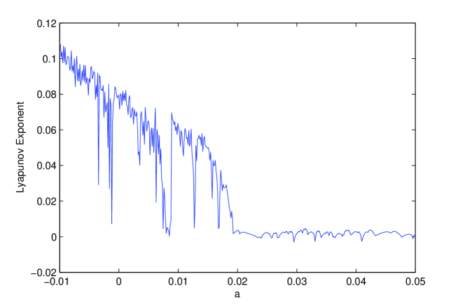
Figure 1: (Color online) The largest Lyapunov exponent versus the parameter $a$.

II.4 The degenerate case of $a=0$ (Sprott E system)

When $a=-0.005$, the system equilibrium is of the regular saddle-focus type; this case of the chaotic system has been studied before therefore will not be discussed here.

When $a=0$, the equilibrium degenerates. It is precisely the Sprott E system listed in Table I (see FIG. 2). The Ši’lnikov homoclinic criterion might be applied to this system to show the existence of chaos, however, but it involves somewhat subtle mathematical arguments.

In this degenerate case, the positive largest Lyapunov exponent of the system (see Table II) still indicates the existence of chaos. In the time domain, FIG. 3 (top part) shows an apparently chaotic waveform of $y(t)$; while in the frequency domain, FIG. 3 (bottom part) shows an apparently continuous broadband spectrum $|y(t)|$. These all prove that the Sprott E system, or the new system (1) with $a=0$, is indeed chaotic.

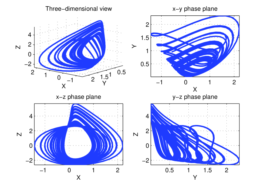
Figure 2: (Color online) The new system: chaotic attractor with $a=0$, including 3D views on the $x$-$y$ plane, $x$-$z$ plane and $y$-$z$ plane.

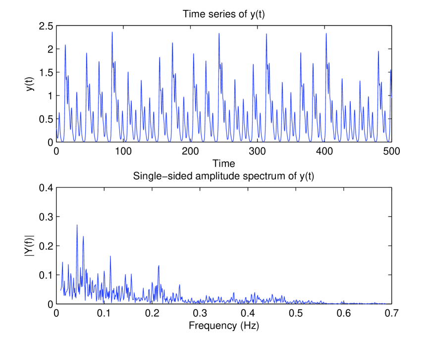
Figure 3: (Color online) Top: An apparently chaotic waveform of $y(t)$ ($a=0$). Bottom: An apparently continuous broadband frequency spectrum $|y(t)|$.

II.5 The case of $a=0.006$: a new type of chaos

When $a>0$, the stability of the equilibrium is fundamentally different from that of the Sprott E system. In this case, the equilibrium becomes a node-focus (see Table II). The Ši’lnikov homoclinic criterion is therefore inapplicable to this case.

Take $a=0.006$ as an example. Numerical calculation of the Lyapunov exponents gives $L_{1}=0.0489$, $L_{2}=0$ and $L_{3}=-1.0485$, indicating the existence of chaos.

In the time domain, FIG. 5 (top part) shows an apparently chaotic waveform $y(t)$; while in the frequency domain, FIG. 5 (bottom part) shows an apparently continuous broadband spectrum $|y(t)|$. These all prove that the new system (1) with $a=0.006$ is indeed chaotic.

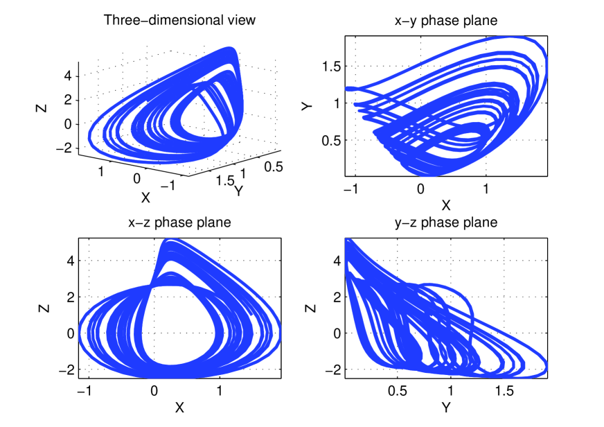
Figure 4: (Color online) The new system: chaotic attractor with $a=0.006$, including 3D views on the $x$-$y$ plane, $x$-$z$ plane and $y$-$z$ plane.

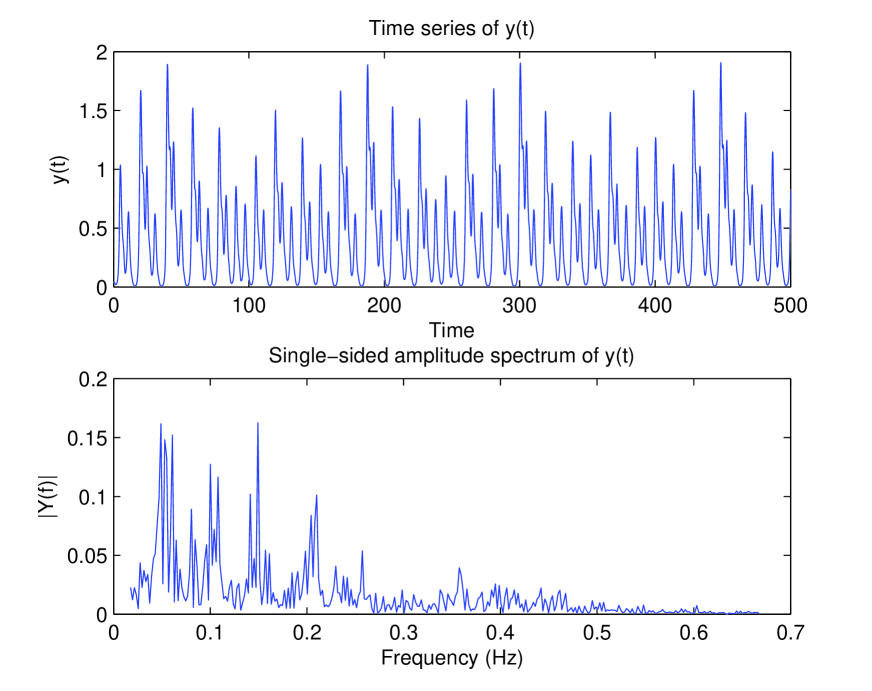
Figure 5: (Color online) Top: An apparently chaotic waveform of $y(t)$ ($a=0.006$). Bottom: An apparently continuous broadband frequency spectrum $|y(t)|$.

II.6 Bifurcations analysis

FIG. 6 shows a bifurcation diagram versus the parameter $a$, demonstrating a period-doubling route to chaos.

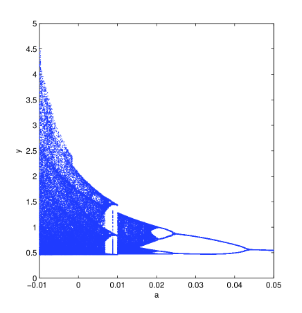
Figure 6: (Color online) Bifurcation diagram, showing a period-doubling route to chaos in $y$ (at $x=0.25$) versus the parameter $a$.

FIG. 7 also demonstrates the gradual evolving dynamical process as $a$ is continuously varied.

Both figures indicate that although the equilibrium is changed from an unstable saddle-focus to a stable node-focus, the chaotic dynamics survive in a relative narrow range of the parameter $a$.

All the above numerical results are summarized in Table III.

Table 3: Numerical results for some values of the parameter $a$ with initial values $(1,1,1)$.

Parameters	Eigenvalues	Lyapunov Exponents	Fractal Dimensions
$a=-0.005$	$\lambda_{1}=-1.03140$	$L_{1}=0.0884$
	$\lambda_{2,3}=0.01570\pm 0.49208i$	$L_{2}=0$	$D_{L}=2.081$
		$L_{3}=-1.0884$
$a=0$	$\lambda_{1}=-1$	$L_{1}=0.0766$
	$\lambda_{2,3}=\pm 0.5i$	$L_{2}=0$	$D_{L}=2.071$
		$L_{3}=-1.0766$
$a=0.006$	$\lambda_{1}=-0.96069$	$L_{1}=0.0510$
	$\lambda_{2,3}=-0.01966\pm 0.50975i$	$L_{2}=0$	$D_{L}=2.048$
		$L_{3}=-1.0510$
$a=0.022$	$\lambda_{1}=-0.84580$	$L_{1}=0$
	$\lambda_{2,3}=-0.07710\pm 0.53818i$	$L_{2}=-0.1381$	$D_{L}=1.000$
		$L_{3}=-0.8619$
$a=0.030$	$\lambda_{1}=-0.78217$	$L_{1}=0$
	$\lambda_{2,3}=-0.10891\pm 0.55476i$	$L_{2}=-0.0826$	$D_{L}=1.000$
		$L_{3}=-0.9174$
$a=0.050$	$\lambda_{1}=-0.60746$	$L_{1}=0$
	$\lambda_{2,3}=-0.19627\pm 0.61076i$	$L_{2}=-0.0518$	$D_{L}=1.001$
		$L_{3}=-0.9482$

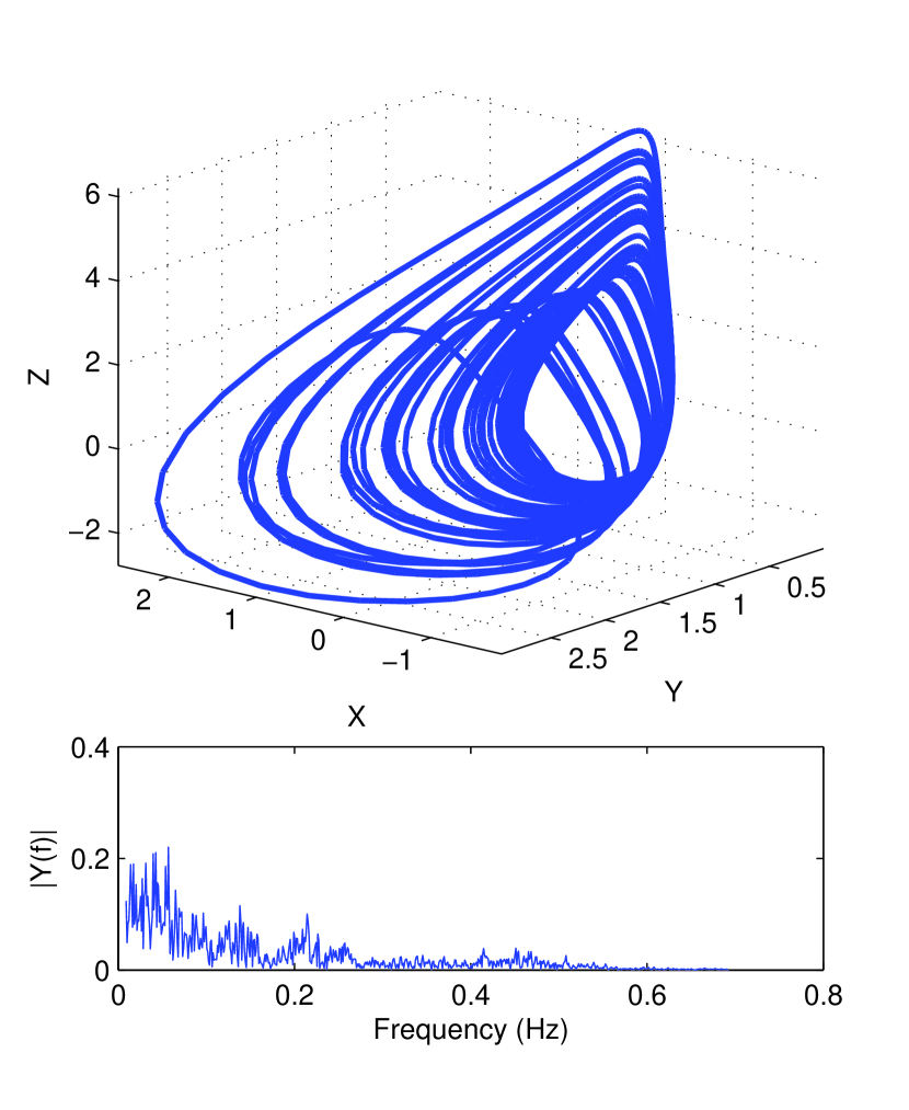
(a)

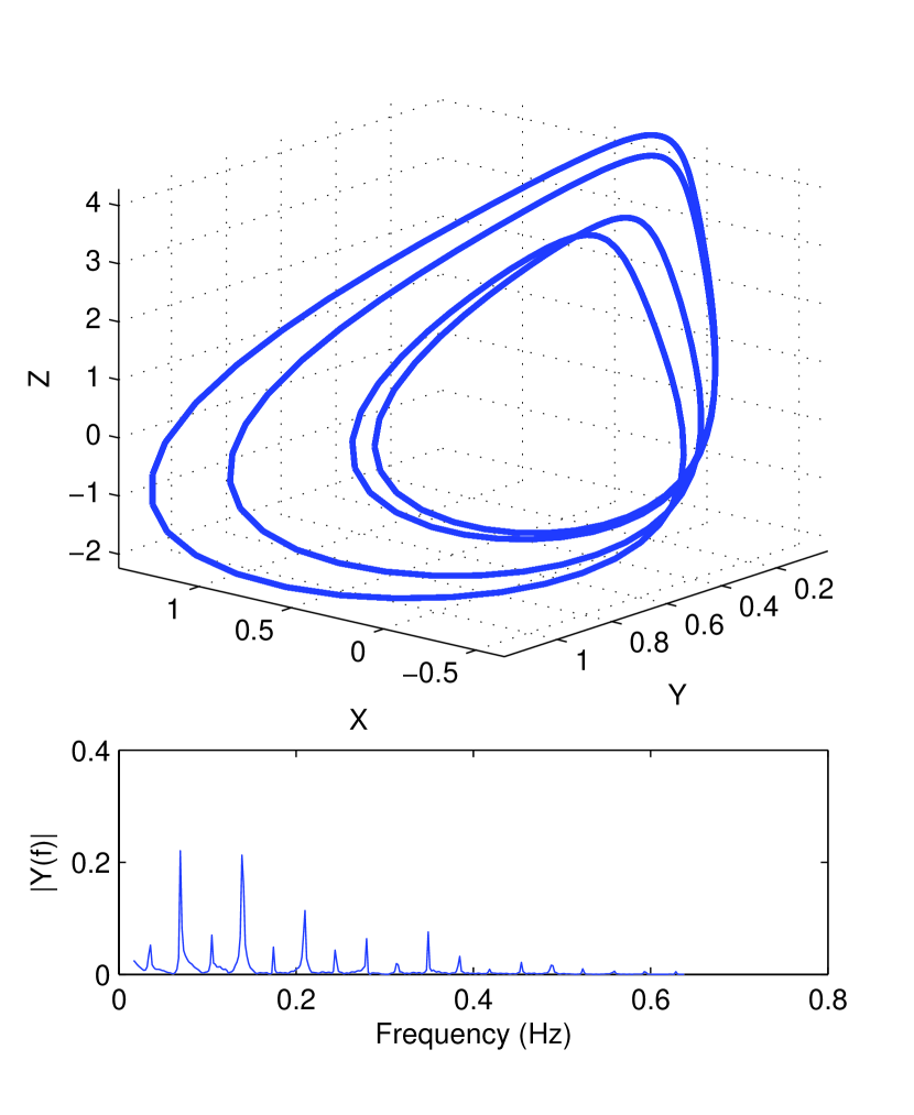
(b)

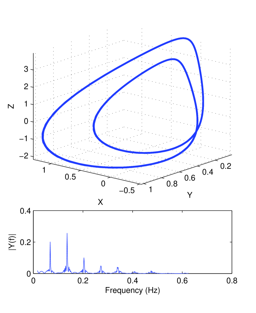
(c)

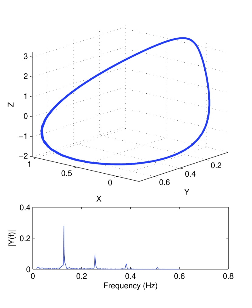
(d)

Figure 7: (Color online) Phase portraits and frequency spectrums: (a) $a=0.006$, (b) $a=0.022$, (c) $a=0.03$, (d) $a=0.05$.

III Conclusion

This paper has reported the finding of a simple three-dimensional autonomous chaotic system which, very surprisingly, has only one stable node-focus equilibrium. The discovery of this new system is striking, because with a single stable equilibrium in a 3D autonomous quadratic system, one typically would anticipate non-chaotic and even asymptotically converging behaviors. Yet, unexpectedly, this system is chaotic. Although the new system is non-hyperbolic type, therefore the Ši’lnikov homoclinic criterion is not applicable, it has been verified to be chaotic in the sense of having a positive largest Lyapunov exponent, a fractional dimension, a continuous frequency spectrum, and a period-doubling route to chaos.

Although the fundamental chaos theory for autonomous dynamical systems seems to have reached its maturity today, our finding reveals some new mysterious features of chaos.

Acknowledgement

This research was supported by the National Natural Science Foundation of China under grant 10832006 and the Hong Kong Research Grants Council under grant CityU1117/10E.

References

- (1) L. Ovsyannikov and L. Shil’nikov, Sbornik: Mathematics 58, 557 (1987).
- (2) L. Šil’nikov, Sbornik: Mathematics 10, 91 (1970).
- (3) A. Šhil’nikov, L. Šhil’nikov, and D. Turaev, Int. J. Bifurcation Chaos, 3, 1123 (1993).
- (4) L. Šhilnikov, A. Šhil’nikov, and D. Turaev, Methods of Qualitative Theory in Nonlinear Dynamics, World Scientific Pub. Co. (2001).
- (5) B. Chen, T. Chen, and G. Chen, Int. J. Bifurcation Chaos, 19, 1679 (2009).
- (6) T. Chen, Y. Tang and G. Chen, Int. J. Bifurcation Chaos, 16, 2459 (2006).
- (7) J. C. Sprott, Comput. and Graphics 17, 325 (1993).
- (8) J. C. Sprott, Phys. Rev. E 50, 647 (1994).
- (9) J. C. Sprott, Phys. Lett. A 228, 271 (1997).
- (10) J. C. Sprott and S. J. Linz, Int. J. Chaos Theory Appl. 5, 3 (2000).
- (11) Q. Yang and G. Chen, Int. J. Bifurcation Chaos 18, 1393 (2008).
- (12) Q. Yang, Z. Wei, and G. Chen, Int. J. Bifurcation Chaos 20, 1061 (2010).