Self-Indexing Based on LZ77

Abstract

We introduce the first self-index based on the Lempel-Ziv 1977 compression format (LZ77). It is particularly competitive for highly repetitive text collections such as sequence databases of genomes of related species, software repositories, versioned document collections, and temporal text databases. Such collections are extremely compressible but classical self-indexes fail to capture that source of compressibility. Our self-index takes in practice a few times the space of the text compressed with LZ77 (as little as 2.6 times), extracts 1–2 million characters of the text per second, and finds patterns at a rate of 10–50 microseconds per occurrence. It is smaller (up to one half) than the best current self-index for repetitive collections, and faster in many cases.

1 Introduction and Related Work

Self-indexes [23] are data structures that represent a text collection in compressed form, in such a way that not only random access to the text is supported, but also indexed pattern matching. Invented in the past decade, they have been enormously successful to drastically reduce the space burden posed by general text indexes such as suffix trees or arrays. Their compression effectiveness is usually analyzed under the $k$-th order entropy model [19]: $H_{k}(T)$ is the $k$-th order entropy of text $T$, a lower bound to the bits-per-symbol compression achievable by any statistical compressor that models symbol probabilities as a function of the $k$ symbols preceding it in the text. There exist self-indexes able to represent a text $T_{1,n}$ over alphabet $[1,\sigma]$, within $nH_{k}(T)+o(n\log\sigma)$ bits of space for any $k\leq\alpha\log_{\sigma}n$ and constant $\alpha<1$ [8, 7].

This $k$-th order entropy model is adequate for many practical text collections. However, it is not a realistic lower bound model for a kind of collections that we call highly repetitive. This is formed by sets of strings that are mostly near-copies of each other. For example, versioned document collections store all the history of modifications of the documents. Most new versions are minor edits of a previous version. Good examples are the Wikipedia database and the Internet archive. Another example are software repositories, which store all the versioning history of software pieces. Again, except for major releases, most versions are minor edits of previous ones. In this case the versioning has a tree structure more than a linear sequence of versions. Yet another example comes from bioinformatics. Given the sharply decreasing sequencing costs, large sequence databases of individuals of the same or closely related species are appearing. The genomes of two humans, for example, share 99.9% to 99.99% of their sequence. No clear structure such as a versioning tree is apparent in the general case.

If one concatenates two identical texts, the statistical structure of the concatenation is almost the same as that of the pieces, and thus the $k$-th order entropy does not change. As a consequence, some indexes that are exactly tailored to the $k$-th order entropy model [8, 7] are insensitive to the repetitiveness of the text. Mäkinen et al. [29, 18] found that even the self-indexes that can compress beyond the $k$-th order entropy model [28, 22] failed to capture most of the repetitiveness of such text collections.

Note that we are not aiming simply at representing the text collections to offer extraction of individual documents. This is relatively simple as it is a matter of encoding the edits with respect to some close sampled version; more sophisticated techniques have been however proposed for this goal [15, 16, 14]. Our aim is more ambitious: self-indexing the collection means providing not only access but indexed searching, just as if the text was available in plain form. Other restricted goals such as compressing the inverted index (but not the text) on natural-language text collections [10] or indexing text $q$-grams and thus fixing the pattern length in advance [5] have been pursued as well.

Mäkinen et al. [29, 18] demonstrated that repetitiveness in the text collections translates into runs of equal letters in its Burrows-Wheeler transform [4] or runs of successive values in the $\Psi$ function [9]. Based on this they engineered variants of FM-indexes [7] and Compressed Suffix Arrays (CSAs) [28] that take advantage of repetitiveness. Their best structure, the Run-Length CSA (RLCSA) still stands as the best general-purpose self-index, despite of some preliminary attempts of self-indexing based on grammar compression [5].

However, Mäkinen et al. showed that their new self-indexes were very far (by a factor of 10) from the space that can be achieved by a compressor based on the Lempel-Ziv 1977 format (LZ77) [30]. They showed the runs model is intrinsically inferior to the LZ77 model to capture repetitions. The LZ77 compressor is particularly able to capture repetitiveness, as it parses the text into consecutive maximal phrases so that each phrase appears earlier in the text. A self-index based on LZ77 was advocated as a very promising alternative approach to the problem.

Designing a self-index based on LZ77 is challenging. Even accessing LZ77-compressed text at random is a difficult problem, which we partially solved [14] with the design of a variant called LZ-End, which compresses only slightly less and gives some time guarantees for the access time. There exists an early theoretical proposal for LZ77-based indexing by Kärkkäinen and Ukkonen [12, 11], but it requires to have the text in plain form and has never been implemented. Although it guarantees an index whose size is of the same order of the LZ77 compressed text, the constant factors are too large to be practical. Nevertheless, that index was the first general compressed index in the literature and is the predecessor of all the Lempel-Ziv indexes that followed [22, 6, 27]. These indexes have used variants of the LZ78 compression format [31], which is more tractable but still too weak to capture high repetitiveness [29].

In this paper we face the challenge of designing the first self-index based on LZ77 compression. Our self-index can be seen as a modern variant of Kärkkäinen and Ukkonen’s LZ77 index, which solves the problem of not having the text at hand and also makes use of recent compressed data structures. This is not trivial at all, and involves designing new solutions to some subproblems where the original solution [12] was too space-consuming. Some of the solutions might have independent interest.

Our resulting index is competitive in theory and in practice. Let $n^{\prime}$ be the number of phrases of the LZ-parsing of $T_{1,n}$. Then a Lempel-Ziv compressor output has size $|LZ|=n^{\prime}(2\log n+\log\sigma)$ (our logarithms are base 2 by default). The size of our LZ77 self-index is at most $2|LZ|+o(|LZ|)$. It can determine the existence of pattern $p_{1,m}$ in $T$ in time $O(m^{2}h+m\log n^{\prime})$, where $h\leq n^{\prime}$ is a measure of the nesting of the parsing (i.e., how many times a character is transitively copied), usually a small number. After this check, each occurrence is reported in time $O(\log n^{\prime}+\delta\log\delta)$, where $\delta$ is another usually small number depending on the nesting of the parsing.

We implemented our self-index over LZ77 and LZ-End parsings, and compared it with the state of the art on a number of real-life repetitive collections consisting of Wikipedia versions, versions of public software, periodic publications, and DNA sequence collections. We have left a public repository with those repetitive collections in http://pizzachili.dcc.uchile.cl/ repcorpus.html, so that standardized comparisons are possible. Our implementations and those of the RLCSA are also available in there.

Our experiments show that in practice the smallest-space variant of our index takes 2.5–4.0 times the space of a LZ77-based compressor, it can extract 1–2 million characters per second, and locate each occurrence of a pattern of length 10 in 10–50 microseconds. Compared to the state of the art (RLCSA), our self-index always takes less space, less than a half on our DNA and Wikipedia corpus. Searching for short patterns is faster than on the RLCSA. On longer patterns our index offers competitive space/time trade-offs.

2 Direct Access to LZ-Compressed Texts

Let us first recall the classical LZ77 parsing [30], as well as the recent LZ-End parsing [14]. This involves defining what is a phrase and its source, and the number $n^{\prime}$ of phrases.

Definition 1 ([30])

The LZ77 parsing of text $T_{1,n}$ is a sequence $Z[1,n^{\prime}]$ of phrases such that $T=Z[1]Z[2]\ldots Z[n^{\prime}]$, built as follows. Assume we have already processed $T_{1,i-1}$ producing the sequence $Z[1,p-1]$. Then, we find the longest prefix $T_{i,i^{\prime}-1}$ of $T_{i,n}$ which occurs in $T_{1,i-1}$, set $Z[p]=T_{i,i^{\prime}}$ and continue with $i=i^{\prime}+1$. The occurrence in $T_{1,i-1}$ of prefix $T_{i,i^{\prime}-1}$ is called the source of the phrase $Z[p]$.

Definition 2 ([14])

The LZ-End parsing of text $T_{1,n}$ is a sequence $Z[1,n^{\prime}]$ of phrases such that $T=Z[1]Z[2]\ldots Z[n^{\prime}]$, built as follows. Assume we have already processed $T_{1,i-1}$ producing the sequence $Z[1,p-1]$. Then, we find the longest prefix $T_{i,i^{\prime}-1}$ of $T_{i,n}$ that is a suffix of $Z[1]\ldots Z[q]$ for some $q<p$, set $Z[p]=T_{i,i^{\prime}}$ and continue with $i=i^{\prime}+1$.

We will store $Z$ in a particular way that enables efficient extraction of any text substring $T_{s,e}$. This is more complicated than in our previous proposal [14] because these structures will be integrated into the self-index later. First, the last characters of the phrases, $T_{i^{\prime}}$ of $Z[p]=T_{i,i^{\prime}}$, are stored in a string $L_{1,n^{\prime}}$. Second, we set up a bitmap $B_{1,n}$ that will mark with a 1 the ending positions of the phrases in $T_{1,n}$ (or, alternatively, the positions where the successive symbols of $L$ lie in $T$). Third, we store a bitmap $S_{1,n+n^{\prime}}$ that describes the structure of the sources in $T$, as follows. We traverse $T$ left to right, from $T_{1}$ to $T_{n}$. At step $i$, if there are $k$ sources starting at position $T_{i}$, we append $1^{k}0$ to $S$ ($k$ may be zero). Empty sources (i.e., $i=i^{\prime}$ in $Z[p]=T_{i,i^{\prime}}$) are assumed to lie just before $T_{1}$ and appended at the beginning of $S$, followed by a 0. So the 0s in $S$ correspond to text positions, and the 1s correspond to the successive sources, where we assume that those that start at the same point are sorted by shortest length first. Finally, we store a permutation $P[1,n^{\prime}]$ that maps targets to sources, that is, $P[i]=j$ means that the source of the $i$th phrase starts at the position corresponding to the $j$th 1 in $S$. Fig. 1(a) gives an example.

(a) The LZ77 parsing of the string ‘alabar_a_la_alabarda$’, showing the sources of each phrase on top. On the bottom, bitmap $B$ marks the ends of phrases, the bitmap $S$ marks the starting positions of sources, and the permutation $P$ connects phrases to sources.

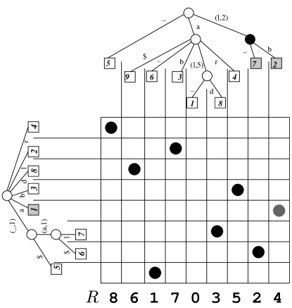
(b) Top: The sparse suffix trie. The black node is the one we arrive at when searching for ‘la’, and the gray leaves of its subtree represent the phrases that start with ‘la’. Left: The reverse trie for the string. The gray leaf is the node at which we stop searching for ‘a’. Bottom: The range structure for the string. The gray circle marks the only primary occurrence of the pattern ‘ala’ (it is the only dot in the range defined by the gray nodes).

Figure 1: Our self-index structure over the example text $T=\texttt{`alabar\_a\_la\_alabarda\$'}$ and part of the process of searching for $p=\texttt{`ala'}$.

The bitmaps $B_{1,n}$ and $S_{1,n+n^{\prime}}$ are sparse, as they have only $n^{\prime}$ bits set. They are stored using a compressed representation [26] so that each takes $n^{\prime}\log\frac{n}{n^{\prime}}+O(n^{\prime})+o(n)$ bits, and rank/select queries are answered in constant time: $rank_{b}(B,i)$ is the number of occurrences of bit $b$ in $B_{1,i}$, and $select_{b}(B,j)$ is the position in $B$ of the $j$th occurrence of bit $b$ (similarly for $S$). The $o(n)$ term, the only one that does not depend linearly on $n^{\prime}$, can disappear at the cost of increasing the time for $rank$ to $O(\log\frac{n}{n^{\prime}})$ [24]. Finally, permutations are stored using a representation [21] that computes $P[i]$ in constant time and $P^{-1}[j]$ in time $O(l)$, using $(1+1/l)n^{\prime}\log n^{\prime}+O(n^{\prime})$ bits of space. We use parameter $l=\log n^{\prime}$. Thus our total space is $n^{\prime}\log n+n^{\prime}\log\frac{n}{n^{\prime}}+n^{\prime}\log\sigma+O(n^{\prime})+o(n)$ bits.

To extract $T_{s,e}$ we proceed as follows. We compute $s^{\prime}=rank_{1}(B,s-1)+1$ and $e^{\prime}=rank_{1}(B,e)$ to determine that we must extract characters from phrases $s^{\prime}$ to $e^{\prime}$. For all phrases except possibly $e^{\prime}$ (where $T_{s,e}$ could end before its last position) we have their last characters in $L[s^{\prime},e^{\prime}]$. For all the other symbols, we must go to the source of each phrase of length more than one and recursively extract its text: to extract the rest of phrase $s^{\prime}\leq k\leq e^{\prime}$, we compute its length as $l=select_{1}(B,k)-select_{1}(B,k-1)$ (except for $k=e^{\prime}$, where the length is $l=e-select_{1}(B,k-1)$) and its starting position as $t=rank_{0}(S,select_{1}(S,P[k]))=select_{1}(S,P[k])-P[k]$. Thus to obtain the rest of the characters of phrase $k$ we recursively extract $T_{t,t+l-1}$

On LZ-End this method takes time $O(e-s+1)$ if $e$ coincides with the end of a phrase [14]. In general, a worst-case analysis [14] yields extraction time $O(e-s+h)$ for LZ-End and $O(h(e-s+1))$ for LZ77, where $h$ is a measure of how nested is the parsing.

Definition 3

Let $T=Z[1]Z[2]\ldots Z[n^{\prime}]$ be a LZ-parsing of $T_{1,n}$. Then the height of the parsing is defined as $h=\max_{1\leq i\leq n}C[i]$, where $C$ is defined as follows. Let $Z[i]=T_{a,b}$ be a phrase whose source is $T_{c,d}$. Then $C[b]=1$ and $C[k]=C[(k-a)+c]+1$ for $a\leq k<b$.

That is, $h$ measures how many times a character is transitively copied in $Z$. While in the worst case $h$ can be as large as $n^{\prime}$, it is usually a small value. It is limited by the longest length of a phrase [13], thus on a text coming from a Markovian source it is $O(\log_{\sigma}n)$. On our repetitive collection corpus $h$ is between 22 and 259 for LZ-End, and between 22 and 1003 for LZ77. Its average values, on the other hand, are 5–25 on LZ-End and 5–176 on LZ77.

Implementation considerations.

As bitmaps $B$ and $S$ are very sparse in highly repetitive collections, we opted for $\delta$-encoding the distances between the consecutive 1s, and adding a sampling where we store the absolute values and position in the $\delta$-codes of every $s$th bit, where $s$ is the sampling rate. So $select$ consists in going to the previous sample and decoding at most $s$ $\delta$-codes, whereas $rank$ requires a previous binary search over the samples.

3 Pattern Searches

Assume we have a text $T$ of length $n$, which is partitioned into $n^{\prime}$ phrases using a LZ77-like compressor. Let $p_{1,m}$ be a search pattern. We call primary occurrences of $p$ those covering more than one phrase or ending at a phrase boundary; and secondary occurrences the others. For example, in Fig. 1(a), the occurrence of ‘lab’ starting at position 2 is primary as it spans two phrases. The second occurrence, starting at position 14, is secondary.

We will find first the primary occurrences, and those will be used to recursively find the secondary ones (which, in turn, will be used to find further secondary occurrences).

3.1 Primary Occurrences

Each primary occurrence can be split as $p=p_{1,i}\,p_{i+1,m}$, where the left side $p_{1,i}$ is a nonempty suffix of a phrase and the (possibly empty) right side $p_{i+1,m}$ is the concatenation of zero or more consecutive phrases plus a prefix of the next phrase. To find primary occurrences we partition the pattern into two in every possible way. Then, we search for the left part in the suffixes of the phrases and for the right part in the prefixes of the suffixes of $T$ starting at phrase boundaries. Then, we find which pairs of left and right occurrences are concatenated, thus representing actual primary occurrences of $p$.

Finding the Right Part of the Pattern.

To find the right side $p_{i+1,m}$ of the pattern we use a suffix trie that indexes all the suffixes of $T$ starting at the beginning of a phrase. In the leaves of the trie we store the identifiers of the phrases where the corresponding suffixes start. Conceptually, the identifiers form an array $id$ that stores the phrase identifiers in lexicographic order of their suffixes. As we see later, we do not need to store $id$ explicitly.

We represent the suffix trie as a Patricia tree [20], encoded using a succinct representation for labeled trees called dfuds [2]. As the trie has at most $2n^{\prime}$ nodes, the succinct representation requires at most $2n^{\prime}\log\sigma+O(n^{\prime})$ bits. It supports a large number of operations in constant time, such as going to a child labeled $c$, going to the leftmost and rightmost descendant leaf, etc. To search for $p_{i+1,m}$ we descend through the tree using the next character of the pattern, skip as many characters as the skip of the branch indicates, and repeat the process until determining that $p_{i+1,m}$ is not in the set or reaching a node or an edge, whose leftmost and rightmost subtree leaves define the interval in array $id$ whose suffixes start with $p_{i+1,m}$. Fig. 1(b) shows on top this trie, shading the range [8,9] of leaves found when searching for $p_{i+1,m}=\texttt{`la'}$.

Recall that, in a Patricia tree, after searching for the positions we need to check if they are actually a match, as some characters are not checked because of the skips.

Instead of doing the check at this point, we defer it for later, when we connect both searches.

We do not explicitly store the skips, as they can be computed from the trie and the text. Given a node in the trie corresponding to a string of length $l$, we go to the leftmost and rightmost leaves and extract the corresponding suffixes since their $(l+1)$th symbols. The number $s$ of symbols they share since that position is the skip. This takes $O(sh)$ time both for LZ77 and LZ-End, since the extraction is from left to right and we have to extract one character at a time until they differ. Thus, the total time for extracting the skips as we descend is $O(mh)$.

Finding the Left Part of the Pattern.

We have another Patricia trie that indexes all the reversed phrases, stored in the same way as the suffix trie. To find the left part of the pattern in the text we search for $(p_{1,i})^{rev}$ in this trie. The array that stores the leaves of the trie is called $rev\_id$ and is stored explicitly. The total space is at most $n^{\prime}\log n^{\prime}+2n^{\prime}\log\sigma+O(n^{\prime})$ bits. Fig. 1(b) shows this trie on the left, with the result of searching for a left part $p_{1,i}=\texttt{`a'}$.

Connecting Both Searches.

Actual occurrences of $p$ are those formed by a phrase $rev\_id[j]=k-1$ and the following one $id[i]=k$, so that $j$ and $i$ belong to the lexicographical intervals found with the tries. To find those we use a $n^{\prime}\times n^{\prime}$ range structure that connects the consecutive phrases in both trees. If $id[i]=k$ and $rev\_id[j]=k-1$, the structure holds a point in $(i,j)$.

The range structure is represented compactly using a wavelet tree [8, 17], which requires $n^{\prime}\log n^{\prime}+O(n^{\prime}\log\log n^{\prime})$ bits. This can be reduced to $n^{\prime}\log n^{\prime}+O(n^{\prime})$ [25]. The wavelet tree stores the sequence $R[1,n^{\prime}]$ so that $R[i]=j$ if $(i,j)$ is a point (note there is only one $j$ per $i$ value). In $O(\log n^{\prime})$ time it can compute $R[i]$, as well as find all the $occ$ points in a given orthogonal range in time $O((occ+1)\log n^{\prime})$. With such an orthogonal range search for the intervals of leaves found in both trie searches, the wavelet tree gives us all the primary occurrences. It also computes any $id[i]=rev\_id[R[i]]+1$ in $O(\log n^{\prime})$ time, thus we do not need to store $id$.

Fig. 1(b) gives an example, showing sequence $R$ at the bottom. It also shows how we find the only primary occurrence of $p=\texttt{`ala'}$ by partitioning it into ‘a’ and ‘la’.

At this stage we also verify that the answers returned by the searches in the Patricia trees are valid. It is sufficient to extract the text of one of the occurrences reported and compare it to $p$, to determine either that all or none of the answers are valid, by the Patricia tree properties.

Note that the structures presented up to now are sufficient to determine whether the pattern exists in the text or not, since $p$ cannot appear if it does not have primary occurrences. If we have to report the $occ$ occurrences, instead, we use bitmap $B$: An occurrence with partition $p_{1,i}$ and $p_{i+1,m}$ found at $rev\_id[j]=k$ is to be reported at text position $select_{1}(B,k)-i+1$.

Overall, the data structures introduced in this section add up to $2n^{\prime}\log n^{\prime}+4n^{\prime}\log\sigma+O(n^{\prime})$ bits. The $occ$ primary occurrences are found in time $O(m^{2}h+m\log n^{\prime}+occ\log n^{\prime})$.

Implementation Considerations.

As the average value for the skips is usually very low and computing them from the text phrases is slow in practice, we actually store the skips using Directly Addressable Codes [3]. These allow storing variable-length codes while retaining fast direct access. In this case arrays $id$ and $rev\_id$ are only accessed for reporting the occurrences.

We use a practical dfuds implementation [1] that binary searches for the child labeled $c$, as the theoretical one [2] uses perfect hashing.

Instead of storing the tries we can do a binary search over the $id$ or $rev\_id$ arrays. This alternative modifies the complexity of searching for a prefix/suffix of $p$ to $O(mh\log n^{\prime})$ for LZ77 or $O((m+h)\log n^{\prime})$ for LZ-End.

Independently, we could store explicitly array $id$, instead of accessing it through the wavelet tree. Although this alternative increases the space usage of the index and does not improve the complexity, it gives an interesting trade-off in practice.

3.2 Secondary Occurrences

Secondary occurrences are found from the primary occurrences and, recursively, from other previously discovered secondary occurrences. The idea is to locate all sources covering the occurrence and then finding their corresponding phrases. Each discovered copy is reported and recursively analyzed for sources containing it.

For each occurrence found $T_{i,i+m-1}$, we find the position pos of the 0 corresponding to its starting position in bitmap $S$, $pos=select_{0}(S,i)$. Then we consider all the 1s to the left of pos, looking for sources that start before the occurrence. For each such $S[j]=1$, $j\leq pos$, the source starts in $T$ at $t=rank_{0}(S,j)$ and is the $s$th source, for $s=rank_{1}(S,j)$. Its corresponding phrase is $f=P^{-1}[s]$, which starts at text position $c=select(B,f-1)+1$. Now we can compute the length of the source, which is the length of its phrase minus one, $l=select_{1}(B,f)-select_{1}(B,f-1)-1$. Finally, if $T_{t,t+l-1}$ covers the occurrence $T_{i,i+m-1}$, then this occurrence has been copied to $T_{c+i-t,c+i-t+m-1}$, where we report a secondary occurrence and recursively find sources covering it. The time per occurrence reported is dominated by that of computing $P^{-1}$, $O(\log n^{\prime})$.

Consider the only primary occurrence of pattern ‘la’ starting at position 2 in our example text. We find the third 0 in the bitmap of sources at position 12. Then we consider all ones starting from position 11 to the left. The 1 at position 11 maps to a phrase of length 2 that covers the occurrence, hence we report an occurrence at position 10. The second 1 maps to a phrase of length 6 that also covers the occurrence, thus we report another occurrence at position 15. The third 1 maps to a phrase of length 1, hence it does not cover the occurrence and we do not report it. We proceed recursively for the occurrences found at positions 10 and 15.

Unfortunately we do not know when to stop looking for 1s to the left in $S$. Stopping as soon as we find the first source not covering the occurrence works only when no source contains another. Kärkkäinen [11] proposes a couple of solutions to this problem, but none is satisfactory in practice.

However, one involves a concept of levels, which we use here in a different way.

Definition 4

Source $s_{1}=[l_{1},r_{1}]$ is said to cover source $s_{2}=[l_{2},r_{2}]$ if $l_{1}<l_{2}$ and $r_{1}\geq r_{2}$.

Let $cover(s)$ be the set of sources covering a source $s$. Then the depth of source $s$ is defined as $depth(s)=0$ if $cover(s)=\emptyset$, and $depth(s)=1+\max_{s^{\prime}\in cover(s)}depth(s^{\prime})$ otherwise. We define $depth(\varepsilon)=0$. Finally, we call $\delta$ the maximum depth in the parsing.

In our example, the four sources ‘a’ and the source ‘alabar’ have depth zero, as all of them start at the same position. Source ‘la’ has depth 1, as it is contained by source ‘alabar’.

We slightly modify the process for traversing $S$ to the left of $pos$. When we find a source not covering the occurrence, we look for its depth $d$ and then consider to the left only sources with depth $d^{\prime}<d$, as those at depth $\geq d$ are guaranteed not to contain the occurrence. This works because sources to the left with the same depth $d$ will end before the current source, and deeper sources to the left will be contained in those of depth $d$. Thus for our traversal we need to solve a subproblem we call $prevLess(D,s,d)$: Let $D[1,n^{\prime}]$ be the array of depths of the sources; given a position $s$ and a depth $d$, we need to find the largest $s^{\prime}<s$ such that $D[s^{\prime}]<d$.

Prev-Less Data Structure.

We represent $D$ using a wavelet tree [8]. This time we need to explain its internal structure. The wavelet tree is a balanced tree where each node represents a range of the alphabet $[0,\delta]$. The root represents the whole range and each leaf an individual alphabet member. Each internal node has two children that split its alphabet range by half. Hence the tree has height $\lceil\log(1+\delta)\rceil$. At the root node, the tree stores a bitmap aligned to $D$, where a 0 at position $i$ means that $D[i]$ is a symbol belonging to the range of the left child, and 1 that it belongs to the right child. Recursively, each internal node stores a bitmap that refers to the subsequence of $D$ formed by the symbols in its range. All the bitmaps are preprocessed for rank/select queries, needed for navigating the tree. The total space is $n^{\prime}\log\delta+O(n^{\prime})$.

We solve $prevLess(D,s,d)$ as follows. We descend on the wavelet tree towards the leaf that represents $d-1$. If $d-1$ is to the left of the current node, then no interesting values can be stored in the right child. So we recursively continue in the left subtree, at position $s^{\prime}=rank_{0}(V,s)$, where $V$ is the bitmap of the current node. Otherwise we descend to the right child, and the new position is $s^{\prime}=rank_{1}(V,s)$. In this case, however, the answer could be at the left child. Any value stored at the left child is $<d$, so we are interested in the rightmost before position $s$. Hence $v_{0}=select_{0}(V,rank_{0}(V,s-1))$ is the last relevant position with a value from the left subtree. We find, recursively, the best answer $v_{1}$ from the right subtree, and return $\max(v_{0},v_{1})$. When the recursion ends at a leaf we return with answer $-1$. The running time is $O(\log\delta)$.

Using this operation we proceed as follows. We keep track of the smallest depth $d$ that cannot cover an occurrence; initially $d=\delta+1$. We start considering source $s$. Whenever $s$ does not cover the occurrence, we set $d=D[s]$ and move to $s^{\prime}=prevLess(D,s,d)$. When $s$ covers the occurrence, we report it and move to $s^{\prime}=prevLess(D,s,d)$.

In the worst case the first source is at depth $\delta$ and then we traverse level by level, finding in each previous source that however does not contain the occurrence. Therefore the overall time is $O(occ(\log n^{\prime}+\delta\log\delta))$ to find $occ$ secondary occurrences.

Final Bounds.

Overall our data structure requires $2n^{\prime}\log n+n^{\prime}\log n^{\prime}+n^{\prime}\log\delta+5n^{\prime}\log\sigma+O(n^{\prime})+o(n)$ bits, where the last term can be removed as explained (multiplying times by $O(\log n)$). As the Lempel-Ziv compressor output has $n^{\prime}(2\log n+\log\sigma)$ bits, the index is asymptotically at most twice the size of the compressed text (for $\log\sigma=o(\log n)$; 3 times otherwise). In practice $\delta$ is much smaller: it is also limited by the maximum phrase length, thus on Markovian sources it is $O(\log_{\sigma}n)$, and in our test collections it is at most 46 and on average 2–4.

Our time to locate the $occ$ occurrences of $p_{1,m}$ is $O(m^{2}h+m\log n^{\prime}+occ(\log n^{\prime}+\delta\log\delta))$.

4 Experimental Evaluation

From the testbed in http://pizzachili.dcc.uchile.cl/repcorpus.html we have chosen four real collections representative of distinct applications: Cere (37 DNA sequences of Saccharomyces Cerevisiae), Einstein (the version of the Wikipedia article on Albert Eintein up to Jan 12, 2010), Kernel (the 36 versions 1.0.x and 1.1.x of the Linux Kernel), and Leaders (pdf files of the CIA World Leaders report, from Jan 2003 to Dec 2009, converted with pdftotext).

We have studied 5 variants of our indexes, from most to least space consuming: (1) with suffix and reverse trie; (2) binary search on explicit $id$ array and reverse trie; (3) suffix trie and binary search on $rev\_id$; (4) binary search on explicit $id$ array and on $rev\_id$; (5) binary search on implicit $id$ and on $rev\_id$. In addition we test parsings LZ77 and LZ-End, so for example LZ-End₃ means variant (3) on parsing LZ-End.

Table 1 gives statistics about the texts, with the compression ratios achieved with a good Lempel-Ziv compressor (p7zip, www.7-zip.org), grammar compressor (repair, www.cbrc.jp/ ~rwan/en/restore.html), Burrows-Wheeler compressor (bzip2, www.bzip.org), and statistical high-order compressor (ppmdi, pizzachili.dcc.uchile.cl/utils/ppmdi.tar.gz). Lempel-Ziv and grammar-based compressors capture repetitiveness, while the Burrows-Wheeler one captures only some due to the runs, and the statistical one is blind to repetitiveness. Then we give the space required by the RLCSA alone (which can count how many times a pattern appears in $T$ but cannot locate the occurrences nor extract text at random), and RLCSA using a sampling of 512 (the minimum space that gives reasonable times for locating and extraction). Finally we show the most and least space consuming of our variants over both parsings.

Our least-space variants take 2.5–4.0 times the space of p7zip, the best LZ77 compressor we know of and the best-performing in our dataset. They are also always smaller than RLCSA₅₁₂ (up to 6.6 times less) and even competitive with the crippled self-index RLCSA-with-no-sampling. The case of Einstein is particularly illustrative. As it is extremely compressible, it makes obvious how the RLCSA achieves much compression in terms of the runs of $\Psi$, yet it is unable to compress the sampling despite many theoretical efforts [18]. Thus even a sparse sampling has a very large relative weight when the text is so repetitive. The data our index needs for locating and extracting, instead, is proportional to the compressed text size.

Collection	Size	p7zip	repair	bzip2	ppmdi	RLCSA	RLCSA512	LZ775	LZ771	LZ-End5	LZ-End1
Cere	440MB	1.14%	1.86%	2.50%	24.09%	7.60%	8.57%	3.74%	5.94%	6.16%	8.96%
Einstein	446MB	0.07%	0.10%	5.38%	1.61%	0.23%	1.20%	0.18%	0.30%	0.32%	0.48%
Kernel	247MB	0.81%	1.13%	21.86%	18.62%	3.78%	4.71%	3.31%	5.26%	5.12%	7.50%
Leaders	45MB	1.29%	1.78%	7.11%	3.56%	3.32%	4.20%	3.85%	6.27%	6.44%	9.63%

Table 1: Space statistics of our texts.

Fig. 2 shows times for extracting snippets and for locating random patterns of length 10. We test RLCSA with various sampling rates (smaller rate requires more space). It can be seen that our LZ-End-based index extracts text faster than the RLCSA, while for LZ77 the results are mixed. For locating, our indexes operate within much less space than the RLCSA, and are simultaneously faster in several cases. See the extended version [13] for more results.

Figure 2: Time performance on the four collections. On the left, extraction speed as a function of the extracted snippet size (higher is better). On the right, time per located occurrence for $m=10$ as a function of the space used by the index, in percentage of text size (lower and leftwards is better). On the right the points for RLCSA refer to different sampling rates; for LZ77 and LZ-End refer to the 5 variants (LZ₅ is leftmost, LZ₁ is rightmost).

5 Conclusions

We have presented the first self-index based on LZ77 compression, showing it is particularly effective on highly repetitive text collections, which arise in several applications. The new indexes improve upon the state of the art in most aspects and solve an interesting standing challenge. Our solutions to some subproblems, such as that of $prevLess$, may be of independent interest.

Our construction needs 6–8 times the original text size and indexes 0.2–2.0 MB/sec. While this is usual in self-indexes and better than the RLCSA, it would be desirable to build it within compressed space.

Another important challenge is to be able to restrict the search to a range of document numbers, that is, within a particular version, time frame, or version subtree. Finally, dynamizing the index, so that at least new text can be added, would be desirable.

References

- [1] D. Arroyuelo, R. Cánovas, G. Navarro, K. Sadakane. Succinct trees in practice. ALENEX, p. 84–97, 2010.
- [2] D. Benoit, E. Demaine, I. Munro, R. Raman, V. Raman, S. Rao. Representing trees of higher degree. Algorithmica, 43(4):275–292, 2005.
- [3] N. Brisaboa, S. Ladra, G. Navarro. Directly addressable variable-length codes. SPIRE, p. 122–130, 2009.
- [4] M. Burrows, D. Wheeler. A block sorting lossless data compression algorithm. TRep. 124, DEC, 1994.
- [5] F. Claude, A. Fariña, M. Martínez-Prieto, G. Navarro. Compressed -gram indexing for highly repetitive biological sequences. BIBE, p. 86–91, 2010.
- [6] P. Ferragina, G. Manzini. Indexing compressed text. J. ACM, 52(4):552–581, 2005.
- [7] P. Ferragina, G. Manzini, V. Mäkinen, G. Navarro. Compressed representations of sequences and full-text indexes. ACM Trans. Alg., 3(2):article 20, 2007.
- [8] R. Grossi, A. Gupta, J. Vitter. High-order entropy-compressed text indexes. SODA, p. 841–850, 2003.
- [9] R. Grossi, J. Vitter. Compressed suffix arrays and suffix trees with applications to text indexing and string matching. STOC, p. 397–406, 2000.
- [10] J. He, J. Zeng, T. Suel. Improved index compression techniques for versioned document collections. CIKM, p. 1239–1248, 2010.
- [11] J. Kärkkäinen. Repetition-Based Text Indexes. PhD thesis, Univ. Helsinki, Finland, 1999.
- [12] J. Kärkkäinen, E. Ukkonen. Lempel-Ziv parsing and sublinear-size index structures for string matching. WSP, p. 141–155, 1996.
- [13] S. Kreft. Self-Index based on LZ77. MSc thesis, Univ. of Chile, 2010. http://www.dcc.uchile.cl/gnavarro/ algoritmos/tesisKreft.pdf.
- [14] S. Kreft, G. Navarro. LZ77-like compression with fast random access. DCC, p. 239–248, 2010.
- [15] S. Kuruppu, B. Beresford-Smith, T. Conway, J. Zobel. Repetition-based compression of large DNA datasets. RECOMB, 2009. Poster.
- [16] S. Kuruppu, S. Puglisi, J. Zobel. Relative Lempel-Ziv compression of genomes for large-scale storage and retrieval. SPIRE, p. 201–206, 2010.
- [17] V. Mäkinen, G. Navarro. Rank and select revisited and extended. Theo.Comp.Sci., 387(3):332–347, 2007.
- [18] V. Mäkinen, G. Navarro, J. Sirén, N. Välimäki. Storage and retrieval of highly repetitive sequence collections. J. Comp. Biol., 17(3):281–308, 2010.
- [19] G. Manzini. An analysis of the Burrows-Wheeler transform. J. ACM, 48(3):407–430, 2001.
- [20] D. Morrison. PATRICIA-Practical algorithm to retrieve information coded in alphanumeric. J. ACM, 15(4):514–534, 1968.
- [21] I. Munro, R.Raman, V.Raman, S.Rao. Succinct representations of permutations. ICALP, p. 345-356, 2003.
- [22] G. Navarro. Indexing text using the Ziv-Lempel trie. J. Discr. Alg., 2(1):87–114, 2004.
- [23] G. Navarro, V. Mäkinen. Compressed full-text indexes. ACM Comp. Surv., 39(1):article 2, 2007.
- [24] D. Okanohara, K. Sadakane. Practical entropy-compressed rank/select dictionary. ALENEX, 2007.
- [25] M. Pǎtraşcu. Succincter. FOCS, p. 305–313, 2008.
- [26] R. Raman, V. Raman, S. Rao. Succinct indexable dictionaries with applications to encoding -ary trees and multisets. SODA, p. 233–242, 2002.
- [27] L. Russo, A. Oliveira. A compressed self-index using a Ziv-Lempel dictionary. Inf. Retr., 5(3):501–513, 2008.
- [28] K. Sadakane. New text indexing functionalities of the compressed suffix arrays. J.Alg., 48(2):294 – 313, 2003.
- [29] J. Sirén, N. Välimäki, V. Mäkinen, G. Navarro. Run-length compressed indexes are superior for highly repetitive sequence collections. SPIRE, p. 164–175, 2008.
- [30] J. Ziv, A. Lempel. A universal algorithm for sequential data compression. IEEE Trans. Inf. Theo., 23(3):337–343, 1977.
- [31] J. Ziv, A. Lempel. Compression of individual sequences via variable-rate coding. IEEE Trans. Inf. Theo., 24(5):530–536, 1978.