The Impact of Incomplete Information on Games in Parallel Relay Networks

Abstract

We consider the impact of incomplete information on incentives for node cooperation in parallel relay networks with one source node, one destination node, and multiple relay nodes. All nodes are selfish and strategic, interested in maximizing their own profit instead of the social welfare. We consider the practical situation where the channel state on any given relay path is not observable to the source or to the other relays. We examine different bargaining relationships between the source and the relays, and propose a framework for analyzing the efficiency loss induced by incomplete information. We analyze the source of the efficiency loss, and quantify the amount of inefficiency which results.

I Introduction

There is now widespread awareness of the importance of incentives in the management of communication networks [1, 2, 3, 4, 5, 6]. Network nodes often cannot be relied upon to cooperatively implement network algorithms in the service of the social good. Instead, selfish nodes will behave in a given manner only if it is profitable for them to do so. Of clear interest is the impact of such selfish actions on the social good. From the network point of view, it is important to design incentives such as pricing schemes, which induce selfish behavior aligned with the social good.

In single-hop networks, the incentive issue and its impact on social efficiency have been extensively studied. In [7, 8], the authors considered the Nash Equilibrium for selfish routing, in which source packets choose paths to the destination to minimize their individual latency, rather than complying with a global routing algorithm to achieve social optimality. In [9] and [10], the authors consider network service pricing for internet service providers. They showed that cooperation among multiple service providers is required when their links are used by common users. In [11], the authors study competitive behavior among multiple parallel links, and characterized the efficiency loss due to competition.

The issue of incentives has also been investigated for multi-hop networks. A number of papers [12, 13, 14] advocate the use of credits to provide incentives for network nodes to cooperate. In [15], the authors investigate the impact of heterogeneous traffic on the pricing of network service providers. Selfish behavior has also been investigated in the context of cooperative relay networks. In [16], the authors considered a nonlinear pricing game, where the relay nodes propose nonlinear charging functions to the source, and the source allocates the traffic to minimize the payment to relay nodes. In [17], the authors considered a Stackelberg bargaining game, in which the relay nodes cooperate as one party in competing with the source node.

All the above papers assume a complete information setting where players in the network game have complete knowledge about quantities such as the state of network links. In practice, this assumption is often too strong. Information regarding network quantities is typically incomplete and imperfect. In an internet service provider (ISP) pricing game, for instance, the characteristics and service requirements of the users can be opaque to the service providers [18]. In a multi-hop network such as the Internet, a source does not typically have perfect information on the congestion state of links a few hops away [19]. Finally, in wireless networks, the source usually cannot observe or test the channel state from a relay to the destination. Neither can a relay observe the channel state from other relays to the destination. Given the above, it is clear that in analyzing selfish behavior in network settings, the role of incomplete information must be emphasized.

One approach to network design problems with incomplete information is through dominant implementable mechanisms [20]. This idea has been used in the context of spectrum auctions [21] and communication networks [22]. These mechanisms, however, require a centralized authority and extra funding from an outsider. This makes the extension to general multi-hop networks difficult. Another approach, based on the idea of Bayesian Nash Equilibrium, a generalization of the Nash Equilibrium concept, is advocated in [23]. Here, the authors consider selfish routing in a single-hop network, where every source node knows only its own traffic requirement, but has knowledge of the traffic distribution of other sources. While the results in [23] are appealing, it remains unclear how they might extend to the multi-hop network situation.

In this work, we investigate the impact of incomplete information on the problem of pricing and incentives in a two-hop parallel relay network. We consider two scenarios, one in which the source has limited bargaining power and one in which the source has full bargaining power. In the limited bargaining power scenario, the source can only react passively to the relays’ signals, and the game can be considered to be a pricing game. For this case, we show that all Nash Equilibria in the complete information game are efficient, including those induced by linear charging functions. We then characterize the Bayesian Nash Equilibrium for the incomplete information game in which relays propose linear pricing functions, and show that incomplete information can induce inefficiencies, which are exacerbated by asymmetric prior knowledge on the type distribution. Next, in the scenario where the source has full bargaining power, the source is allowed to provide a general contract. For this case, we first show that in the game with complete information, (Bayesian) Nash equilibria exist and are all efficient. Next, we investigate the game with incomplete information. To deal with the difficulty of characterizing the Bayesian Nash Equilibria in this case, we first show that if a resource allocation outcome can be realized by a Bayesian Nash equilibrium, then there exists a “truth telling” Bayesian Nash equilibrium that realizes the outcome. We then show that the set of outcomes for the “truth telling” Bayesian Nash equilibria is included in the set of outcomes for the Nash equilibria for a complete information game, in which the link cost functions are replaced by specified “virtual cost functions.” Using this approach, we obtain for a symmetric network scenario a bound on the amount of inefficiency which may result from incomplete information.

II Network Model

II-A Network Traffic Allocation

In wireline and wireless networks, it is often the case that an information source cannot directly reach its destination, but must do so with the aid of intermediate relays. We model such a situation as follows. Consider a parallel relay network modelled by a directed graph $G=(V,E)$, with a single source $s$, destination $d$, and a set of relays $I$, where $|I|=n$. We assume that there is no direct link between $s$ and $d$. Instead, The relays in $I$ are used to forward traffic in a two-hop fashion from $s$ to $d$.

The source wishes to maintain a certain rate of transmission with the destination. We shall consider two scenarios. In the first inelastic scenario, the source has a fixed rate $r_{s}$ of transmission. This rate must be carried by the relays in $I$, where the traffic rate forwarded by relay $i$ is $r_{i}$, and $\sum_{i=1}^{n}r_{i}=r_{s}$. In the second elastic scenario, the source may be willing to withhold some of its transmission rate, according to how the cost of sending traffic affects it overall utility. Let $r_{0}$ denote the amount of traffic withheld or rejected. Then $r_{s}-r_{0}$ is the total admitted traffic from the source. A traffic vector $\mathbf{r}\triangleq(r_{0},r_{1},\ldots,r_{n})\in{\mathbb{R}}_{+}^{n+1}$ is a feasible routing of the source traffic if it satisfies $r_{0}+\sum_{i=1}^{n}r_{i}=r_{s}$.

II-B Cost Function and Utility Function

In general, for any relay node $i$, there is a cost involved in forwarding traffic for source $s$. This cost typically depends both on the properties of the links adjacent on relay $i$ and the amount of traffic flowing through those links. Denote the traffic flow on link $(i,j)\in E$ by $f_{ij}$. We assume that link $(i,j)$ has a cost function $C_{ij}(\theta_{ij},f_{ij})$ with $C_{ij}(\theta_{ij},0)=0$, where $\theta_{ij}$ is a measure of the quality of link $(i,j)$. This quality may have different physical meanings in different contexts. For example, if the cost function reflects the queuing delay on $(i,j)$, then using the M/M/1 approximation, $C_{ij}(\theta_{ij},f_{ij})=\frac{f_{ij}}{k_{ij}-f_{ij}}$. Here, $\theta_{ij}$ denotes the link capacity $k_{ij}$. For another example, consider the cost of power assumption required for transmitting traffic of rate $f_{ij}$ over a wireless link with channel gain $g_{ij}$, bandwidth $W$, and receiver noise power $N$. Using the Shannon capacity formula, we have $f_{ij}=W\log(1+g_{ij}P_{ij}/N)$, where $P_{ij}$ is transmission power required on link $(i,j)$. Thus, the link cost is

$$C_{ij}(\theta_{ij},f_{ij})=\frac{N}{g_{ij}}(2^{f_{ij}/W}-1).$$

Here, $\theta_{ij}$ denotes the channel gain $g_{ij}$.

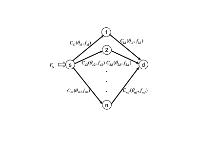
Figure 1: relay channel

Now consider the overall cost $C_{i}(\theta_{i},r_{i})$ for relay node $i$ to forward traffic of rate $r_{i}$ from source $s$ to destination $d$, where $\theta_{i}$ measures the quality or type of the path from $s$ to $d$ through $i$. We assume that $C_{i}(\theta_{i},r_{i})=C_{si}(\theta_{si},r_{i})+C_{id}(\theta_{id},r_{i})$. The costs $C_{i}(\theta_{i},r_{i})$ are particularly amenable to analysis if $\theta_{i}$ can be expressed as a simple scalar function of $\theta_{si}$ and $\theta_{id}$: $\theta_{i}=h(\theta_{si},\theta_{id})$. This is true in the example of the power consumption cost function given above, where $\theta_{ij}=g_{ij}$ is the channel gain on link $(i,j)$. Normalizing the bandwidth and receiver noise power to 1, we have

$$C_{i}(\theta_{i},r_{i}) = P_{si}+P_{id}$$ (1)

$$= (2^{r_{i}}-1)/g_{si}+(2^{r_{i}}-1)/g_{id}$$

$$= (2^{r_{i}}-1)\theta_{i}^{-1},$$

where $\theta_{i}\triangleq(g_{si}^{-1}+g_{id}^{-1})^{-1}=(\theta_{si}^{-1}+\theta_{id}^{-1})^{-1}$. In this paper, we focus on situations where the path quality $\theta_{i}$ can be expressed as a scalar function of $\theta_{si}$ and $\theta_{id}$. We further assume that $\theta_{i}$ belongs to a compact interval $[\underline{\theta}_{i},\overline{\theta}_{i}]$.

Motivated by the power consumption example, we assume that $C_{i}(\theta_{i},r_{i})$ is twice continuously differentiable on $[\underline{\theta}_{i},\overline{\theta}_{i}]\times[0,r_{s}]$, and strictly increasing and convex in $r_{i}$: ${\partial{C_{i}(\theta_{i},r_{i})}}/{\partial{r_{i}}}>0$ and ${\partial^{2}{C_{i}(\theta_{i},r_{i})}}/{\partial{r_{i}^{2}}}>0$. Also, assume that $C_{i}(\theta_{i},r_{i})$ is strictly decreasing in $\theta_{i}$: ${\partial{C_{i}(\theta_{i},r}_{i}{)}}/{\partial{\theta_{i}}}<0$. Furthermore, assume ${\partial^{2}{C_{i}(\theta_{i},r_{i})}}/{\partial{\theta_{i}}\partial{r_{i}}}\leq 0$.

Now consider the source $s$. In the inelastic case, source $s$ sends traffic at a fixed rate $r_{s}$ into the network. In the elastic case, source $s$ may withhold traffic of rate $r_{0}$ from the network, and send the other part of the traffic $r_{s}-r_{0}$ into the network. Let the utility function of the source be given by $W_{s}(\theta_{s},r)$, where $\theta_{s}\in[\underline{\theta}_{s},\overline{\theta}_{s}]$ parameterizes the utility for the source, and $r$ is the source rate admitted into the network. For example, the source utility may be $W_{s}(\theta_{s},r)=\theta_{s}\log(1+r)$. Assume that $W_{s}(r)=W_{s}(r_{s})$ for all $r\geq r_{s}$, i.e. $r_{s}$ is the maximum desired source rate. $W_{s}(\theta_{s},r)$ is assumed to be continuously differentiable, strictly increasing and concave in $r$ on $[0,r_{s}]$. Let $C_{s}(\theta_{s},r_{0})\triangleq W_{s}(r_{s})-W_{s}(r_{s}-r_{0})$ denote the source’s utility loss from having traffic of rate $r_{0}$ withheld from the network. Equivalently, if $r_{0}$ is regarded as the traffic rate routed on a virtual overflow link directly from $s$ to $d$ [19], then $C_{s}(\theta_{s},r_{0})$ represents the cost on the overflow link when the link parameter is $\theta_{s}$ and the flow rate is $r_{0}$. Since $W_{s}(r_{s})$ is a constant, it can be seen that $C_{s}(\theta_{s},r_{0})$ is continuously differentiable on $[\underline{\theta}_{s},\overline{\theta}_{s}]\times[0,r_{s}]$, strictly increasing and convex in $r_{0}$: ${\partial{C}_{s}{(\theta_{s},r_{0})}}/{\partial r{{}_{0}}}>0$ and ${\partial^{2}{C}_{s}{(\theta_{s},r_{0})}}/{\partial r{{}_{0}^{2}}}>0$. Furthermore, we assume that $C_{s}(\theta_{s},r_{0})$ is strictly decreasing in $\theta_{s}$: ${\partial{C}_{s}{(\theta_{s},r_{0})}}/{\partial\theta{{}_{s}}}<0$. Finally, it can be seen that $C_{s}(\theta_{s},0)=0$ for all $\theta_{s}$. It can easily be checked that these properties are satisfied for the example $W_{s}(\theta_{s},r)=\theta_{s}\log(1+r)$, for which $C_{s}(\theta_{s},r_{0})=W_{s}(r_{s})-\theta_{s}\log(1+r_{s}-r_{0})$. With the aid of the virtual overflow link, we may view a game with an elastic source as a game with an inelastic source of rate $r_{s}$ and an overflow link $(s,w)$ with cost function $C_{s}(\theta_{s},r_{0})$.

II-C Socially Optimal Allocation

A socially optimal traffic allocation in a parallel relay network is an allocation which minimizes the total network cost, assumed to be the sum of the link costs. Such an allocation can be realized through cooperation of the network nodes. In networks with selfish and strategic nodes, a socially optimal allocation may or may not be realizable. Nevertheless, the optimal allocation serves as an important benchmark with which to measure the amount of potential inefficiency introduced by selfish and strategic behavior.

Let $R\triangleq\{(r_{0},r_{1},...,r_{n})$$:r_{j}\geq 0~{}\forall j=0,\ldots,n,\sum_{j=0}^{n}r_{j}=r_{s}\}$ be the set of feasible traffic allocations, and let $\mathbf{r}\in R$ denote the vector of traffic rates in the network, where $r_{0}$ is the rate withheld by the source, and $r_{i}$ is the rate routed to relay $i,i=1,\ldots,n$. Note that for the case of an inelastic source, $r_{0}=0$.

Definition 1.

A traffic allocation vector $\mathbf{r}^{*}$ is called socially optimal if

$$\mathbf{r}^{*}\in\arg\min_{\mathbf{r}\in R}C_{s}(\theta_{s},r_{0})+\sum_{i=1}^{n}C_{i}(\theta_{i},r_{i}).$$ (2)

Since the link cost functions $C_{i}(\theta_{i},r_{i})$ as well as $C_{s}(\theta_{s},r_{0})$ are all strictly increasing and strictly convex, the socially optimal allocation $\mathbf{r}^{*}$ exists and is unique. The conditions for specifying $\mathbf{r}^{*}$ can be obtained using the Kuhn-Tucker conditions. Let $c_{i}(\theta_{i},r_{i})\triangleq{\partial{C_{i}(\theta_{i},r_{i})}}/{\partial{r_{i}}}$ and $c_{s}(\theta_{s},r_{0})\triangleq{\partial{C_{s}(\theta_{s},r_{0})}}/{\partial{r_{0}}}$ denote the marginal cost function of link $i$ and the marginal cost function of the overflow link for source $s$, respectively.

For the case of an inelastic source, $\mathbf{r}^{*}=(0,r^{*}_{1},\ldots,r^{*}_{n})$ is the socially optimal allocation if and only if for each $i=1,\ldots,n$,

$$c_{i}(\theta_{i},r^{*}_{i})=c^{*}~{}\text{if}~{}r^{*}_{i}>0,\quad c_{i}(\theta_{i},r^{*}_{i})>c^{*}~{}\text{if}~{}r^{*}_{i}=0.$$ (3)

For the case of an elastic source, $\mathbf{r}^{*}=(r^{*}_{0},r^{*}_{1},\ldots,r^{*}_{n})$ is the socially optimal allocation if and only if (3) holds and furthermore,

$$c_{s}(\theta_{s},r^{*}_{0})=c^{*}~{}\text{if}~{}r^{*}_{0}>0,\quad c_{s}(\theta_{s},r^{*}_{0})>c^{*}~{}\text{if}~{}r^{*}_{0}=0.$$

II-D Game Structure

Unlike the cooperative setting, in a network consisting of selfish and strategic nodes, the source as well as the relays will strategize to maximize their own utility, rather than work together to minimize the overall network cost. Since forwarding traffic entails cost, the relays will carry the source’s traffic only if they are sufficiently well compensated. The source, on the hand, wishes to have its traffic forwarded at the smallest possible cost to itself. The natural setting in which to carry out this game is one which allows for transfer payments which accompany traffic allocations from the source to the respective relays.

In this work, we assume that the (maximum) source input rate $r_{s}$ and the parameter $\theta_{s}$ are known to all nodes. As discussed above, the cost function $C_{i}(\theta_{i},r_{i})$ for relay $i$ depends on the path quality parameter or type $\theta_{i}$. In practical network settings, the value of this type may be randomly fluctuating. For instance, in wireless communication, the channel gain $g_{ij}$ fluctuates due to shadowing and fading. In the Internet, the quality of a particular path may fluctuate according to network congestion levels. Accordingly, we may assume that $\theta_{i}$ is randomly distributed according to distribution function $F_{i}(\theta_{i})$. In practical network scenarios, the exact realization of $\theta_{i}$ is typically known only to relay $i$, and not to the source or to the relays other than $i$. Thus, $\theta_{i}$ is private information to relay $i$. Nevertheless, the source and other relays may still have knowledge of the distribution $F_{i}(\theta_{i})$. For instance, a wireless source or a relay $j\neq i$ may know the distribution of the channel gains for relay $i$, but typically does not know the realization of those channel gains. An Internet source or a path $j\neq i$ may know the distribution of the congestion level on path $i$, but does not know the exact realization of the congestion level.

In order for the source node to allocate its traffic intelligently in the presence of incomplete information regarding the $\theta_{i}$’s, it needs to observe some “signal” from the relay nodes. This can be realized by having the relay node send a signal according to the realization of its type to the source. Let $M_{i}$ be the set of signals for relay $i$, where $M_{i}$ is a subset of the set of differentiable functions on $[0,r_{s}]$. The signal map for relay $i$ is

$$s_{i}:\Theta_{i}\rightarrow M_{i},$$

where $\Theta_{i}\triangleq[\underline{\theta}_{i},\overline{\theta}_{i}]$ and $s_{i}(\theta_{i})=m_{i}(\cdot)$.

Given the signals $m_{i}(\cdot),i=1,\ldots,n$, the source decides on an allocation of its traffic as well as a vector of transfer payments to the relays. This allocation is called a contract. Let $\mathbf{r}=(r_{0},r_{1},...,r_{n})\in R$ denote the vector of traffic rates in the network, where $r_{0}$ is the rate withheld by the source, and $r_{i}$ is the rate routed to relay $i,i=1,\ldots,n$. Note that for the inelastic case, $r_{0}=0$. Now let $\mathbf{t}=(t_{1},t_{2},...,t_{n})\in{\mathbb{R}}_{+}^{n}$ be the vector of transfer payments, where $t_{i}$ is the transfer payment to relay $i$. Let $M\triangleq M_{1}\times\cdots\times M_{n}$ and $T\triangleq{\mathbb{R}}_{+}^{n}$. Then the allocation map of the source node is

$$g:M\rightarrow R\times T,$$

where $g(m_{1}(\cdot),\ldots,m_{n}(\cdot))=(\mathbf{r},\mathbf{t})$.

The above framework encompasses many forms of pricing games explored in previous literature. For instance, in [16], the relay signals are simply charging functions $P_{i}(\cdot)$, and the transfer payments are required to equal the charges demanded by the relays, i.e. $t_{i}=P_{i}(r_{i})$.

The signal maps of the relays along with the allocation map of the source realize a corresponding network allocation map

$$f:\Theta\rightarrow R\times T,$$

where $f(\theta_{1},\ldots,\theta_{n})=g(s_{1}(\theta_{1}),\ldots,s_{n}(\theta_{n}))=(\mathbf{r},\mathbf{t})$.

In the game with incomplete information corresponding to the above setting, the utility of the source is given by

$${U}_{s}(\theta_{s},g(s_{1}(\theta_{1}),\ldots,s_{n}(\theta_{n}))=W_{s}(r_{s})-C_{s}(\theta_{s},r_{0})-\sum_{i=1}^{n}t_{i}.$$

The utility of relay $i$ is given by

$$U_{i}(\theta_{i},g(s_{1}(\theta_{1}),\ldots,s_{n}(\theta_{n})))=t_{i}-C_{i}(\theta_{i},r_{i}).$$

The game with incomplete information proceeds as follows. First, each relay $i$ observes its own private information $\theta_{i}$. Second, the source provides a contract for the relay nodes. The contract announces the source allocation rule $g:M\rightarrow R\times T$. Third, the relays simultaneously decide to either accept or reject the contract. If a given relay accepts the contract, then it will participate in the game which follows. Otherwise, the relay quits and receives zero utility. Fourth and finally, the relay nodes simultaneously send their signals to the source, and the source allocates rates and transfer payments according to the announced $g$.

In the following, we give the formal definition of the Bayesian Nash equilibrium corresponds to the game with incomplete information described above. Let ${\mathbf{\theta}}\triangleq(\theta_{1},\ldots,\theta_{n})$, ${\mathbf{\theta}}_{-i}\triangleq(\theta_{j})_{j\neq i}$, and $s_{-i}({\mathbf{\theta}}_{-i})\triangleq(s_{j}(\theta_{j}))_{j\neq i}$.

Definition 2.

A Bayesian Nash Equilibrium of the above game is a set of strategies $\{s_{1},\ldots,s_{n},g\}$ satisfying

• for each relay node $i$ and every feasible $\widetilde{s_{i}}:\Theta_{i}\rightarrow M_{i}$,

  $$E_{\theta_{-i}}\left\{U_{i}(\theta_{i},g(s_{i}(\theta_{i}),s_{-i}(\theta_{-i})))\right\}$$

  $$\geq E_{\theta_{-i}}\left\{U_{i}(\theta_{i},g(\widetilde{s_{i}}(\theta_{i}),s_{-i}(\theta_{-i})))\right\},$$ (4)

• for every feasible $\widetilde{g}:M\rightarrow R\times T$,

  $$E_{\mathbf{\theta}}\left\{U_{s}(\theta_{s},g(s(\mathbf{\theta})))\right\}\geq E_{\mathbf{\theta}}\left\{U_{s}(\theta_{s},\widetilde{g}(s(\mathbf{\theta})))\right\}.$$ (5)

III Games with Limited Source Bargaining Power

We first consider a specific instance of the general game described in Section II-D in which the source has limited bargaining power. In this case, the source can only react passively to the relays’ signals. Specifically, the transfer payment from the source to any given relay must equal the relay’s signal function evaluated at the traffic rates routed to the relay. That is, the source allocation rule is given by $g(m_{1}(\cdot),\ldots,m_{n}(\cdot))=(\mathbf{r},\mathbf{t})$, where

$$\mathbf{r} \in \arg\max_{\mathbf{r}^{\prime}\in R}W_{s}(\theta_{s},r_{s})-C_{s}(\theta_{s},r^{\prime}_{0})-\displaystyle\sum\limits_{i=1}^{n}m_{i}(r_{i}^{\prime})$$ (6)

$$t_{i} = m_{i}(r_{i}),\quad i=1,\ldots,n.$$ (7)

Effectively, the relays’ signal functions act as charging functions, and the transfer payments must correspond to the relays’ charges. The source can only allocate its traffic to minimize the cost of withheld traffic plus the total charges paid to the relays. In this case, the game can be considered to be a pricing game.

III-A Pricing Game with Complete Information

In this section, we consider the specific pricing game with complete information where the source has limited bargaining power and the vector of relay types $\theta=(\theta_{1},\ldots,\theta_{n})$ is known to all nodes in the network. Note that this is degenerate version of the game considered in Section II-D where the prior distribution on the type of relay $i$ available to all nodes is given by the distribution function $F_{i}(x)=0$ for $x<\theta_{i}$ and $F_{i}(x)=1$ for $x\geq\theta_{i}$, where $\theta_{i}$ is the realization of relay $i$’s type.

Since the allocation rule of the source is fixed by (6)-(7), the knowledge of $\theta$ cannot cause the source to adjust its allocation rule accordingly. Thus, knowledge of $\theta$ is not useful to the source due to its lack of bargaining power. Also, due to the degenerate prior distribution on $\theta_{i}$, we need only consider the usual concept of Nash equilibrium here. We now show that in fact all the Nash equilibria in this complete information pricing game are efficient.

Theorem 1.

In the pricing game with complete information, Nash equilibria exist, and all Nash equilibria are efficient. Moreover, there exists an efficient Nash equilibrium in which each relay uses a linear charging function.

Proof.

We focus on the case for inelastic sources. The elastic case can be similarly handled. Since $\theta=(\theta_{1},\ldots,\theta_{n})$ is known to all nodes in the network, we suppress the dependence of various quantities on $\theta$. In this game with limited source bargaining power, the relays’ signals represent charging functions. Let $B_{i}(r_{i})$ be the charge required by relay $i$ for forwarding traffic of rate $r_{i}$, and let $b_{i}(r_{i})\triangleq B^{\prime}_{i}(r_{i})$ be the marginal charging function, or pricing function. Let $C_{i}(r_{i})$ and $c_{i}(r_{i})$ be cost function and marginal cost function for relay $i$, respectively.

Let the (unique) socially optimal allocation be ${\mathbf{r}}^{*}=(r_{1}^{*},r_{2}^{*},...,r_{n}^{*})$. Suppose that there exists a Nash Equilibrium with charging functions $B_{i}(r_{i})$ and corresponding rate allocation ${\mathbf{r}}=(r_{1},r_{2},...,r_{n})\neq{\mathbf{r}}^{*}$. With a possible re-ordering of the relay indices, we may assume that $r_{i}>r_{i}^{*}$ for $i<k_{1}$, $r_{i}=r_{i}^{*}$ for $k_{1}\leq i<k_{2}$, and $r_{i}<r_{i}^{*}$ for $i\geq k_{2}$. As ${\mathbf{r}}\neq{\mathbf{r}}^{*}$ and both must sum to $r_{s}$, $k_{1}>1$ and $k_{2}<n$.

Since ${\mathbf{r}}^{*}$ is the unique socially optimal allocation, from the optimality conditions, we have

$$c_{i}(r_{i}^{*})=c^{*}~{}\text{if}~{}r^{*}_{i}>0,\quad c_{i}(r_{i}^{*})>c^{*}~{}\text{if}~{}r^{*}_{i}=0.$$ (8)

where $c^{*}$ is the optimal marginal cost. Now by the strict convexity of $C_{i}(r_{i})$,

$$\left\{\begin{array}[]{ll}c_{i}(r)>c^{*}~{}\text{for all}~{}r\in[r^{*}_{i},r_{i})~{}\text{if}~{}i<k_{1}&\\ c_{i}(r)<c^{*}~{}\text{for all}~{}r\in(r_{i},r^{*}_{i}]~{}\text{if}~{}i>k_{2}&\end{array}\right.$$ (9)

The profit of relay $i$ for $i<k_{1}$ is

$$\int_{0}^{r_{i}^{*}}b_{i}(r)-c_{i}(r)dr+\int_{r_{i}^{*}}^{r_{i}}b_{i}(r)-c_{i}(r)dr.$$ (10)

Since we are at a Nash equilibrium, for all $i<k_{1}$ and for any $0<\delta<r_{i}-r_{i}^{*}$, $\int_{r_{i}-\delta}^{r_{i}}b_{i}(r)-c_{i}(r)dr\geq 0$. For otherwise, relay $i<k_{1}$ will deviate to another charging function which is extremely high from $r_{i}^{*}$ to $r_{i}$, so as not to take the extra traffic $r_{i}-r_{i}^{*}$. Now choose $\epsilon<min_{i:i<k_{1}~{}\text{or}~{}i\geq k_{2}}|r_{i}-r_{i}^{*}|$. Let

$$\left\{\begin{array}[]{ll}m&\in\quad\arg\max_{1\leq i<k_{1}}\int_{r_{i}-\epsilon}^{r_{i}}c_{i}(r)dr\\ l&\in\quad\arg\min_{k_{2}\leq i\leq n}\int_{r_{i}}^{r_{i}+\epsilon}c_{i}(r)dr\end{array}\right.$$ (11)

By (9),

$$\int_{r_{m}-\epsilon}^{r_{m}}c_{m}(r)dr>\int_{r_{l}}^{r_{l}+\epsilon}c_{l}(r)dr$$ (12)

However, since $\int_{r_{m}-\epsilon}^{r_{m}}b_{m}(r)-c_{m}(r)dr\geq 0$, there exists a charging function $\tilde{B}_{l}(r)$ for relay $l$ such that $\tilde{B}_{l}(r)$ equals $B_{l}(r)$ from 0 to $r_{l}$, but

$$\begin{array}[]{ll}\int_{r_{m}-\epsilon}^{r_{m}}b_{m}(r)dr&\geq\quad\int_{r_{m}-\epsilon}^{r_{m}}c_{m}(r)dr\\ &>\quad\int_{r_{l}}^{r_{l}+\epsilon}\tilde{b}_{l}(r)dr\quad>\quad\int_{r_{l}}^{r_{l}+\epsilon}c_{l}(r)dr.\end{array}$$ (13)

Thus if relay $l$ uses $\tilde{B}_{l}(r)$, then in order to maximize its profit, the source will switch an $\epsilon$ amount of traffic from relay $m$ to relay $l$. Thus, relay $l$ can deviate to $\tilde{B}_{l}(r)$ and get a higher profit, contradicting our assumption of being at a Nash equilibrium.

The existence of an efficient Nash equilibrium in which relays use linear charging functions has been demonstrated in [16], completing the proof. ∎

III-B  Pricing Game with Incomplete Information

When the source and the relays $j\neq i$ cannot observe the type $\theta_{i}$ of relay $i$, the source and the relays must content themselves with maximizing their expected profits. In this situation, the characterization of Bayesian Nash Equilibria for general nonlinear charging functions is very difficult. We limit our discussion to the case where relays bid linear charging functions, i.e. $B_{i}(\theta_{i},r_{i})=p_{i}(\theta_{i})r_{i}$, where the price $p_{i}(\theta_{i})$ per unit traffic depends on the type $\theta_{i}$. Let $w_{i}\triangleq p_{i}^{-1}$ be the inverse function of $p_{i}$ such that $\theta_{i}=w_{i}(p_{i}(\theta_{i}))$. We assume that the density $f_{i}(\theta_{i})$ is positive over $\Theta_{i}=[\underline{\theta}_{i},\overline{\theta}_{i}]$.

We prove the following theorem.

Theorem 2.

If the source is inelastic, in any Bayesian Nash Equilibrium, the price function satisfies the following differential equations:

$$\frac{dw_{i}(p_{i})}{dp_{i}} = \frac{F_{i}(w_{i}(p_{i}))}{(n-1)f_{i}(w_{i}(p_{i}))}\Bigg{\{}\frac{-(n-2)r_{s}}{p_{i}r_{s}-C_{i}(w_{i}(p_{i}),r_{s})}$$ (14)

$$+\displaystyle\sum\limits_{j\neq i}\frac{r_{s}}{p_{i}r_{s}-C_{j}(w_{j}(p_{i}),r_{s})}\Bigg{\}},$$

where $p_{i}(\theta_{i})$ is given by the inverse of $w_{i}(p_{i})$.

In particular, in the symmetric situation where $F_{i}(\theta_{i})=F(\theta_{i})$ and $C_{i}(\theta_{i},r_{i})=C(\theta_{i},r_{i})$ for all $i$, the Bayesian Nash Equilibrium satisfies:

$$p_{i}(\theta_{i})=\frac{1}{r_{s}}\left\{C(\theta_{i},r_{s})-\frac{\int_{\underline{\theta}}^{\theta_{i}}F(\theta)^{n-1}\frac{\partial C(\theta,r_{s})}{\partial\theta}d\theta}{F(\theta_{i})^{n-1}}\right\}.$$ (15)

Proof.

By an argument similar to that in [24], $p_{i}(\theta_{i})$ and $w_{i}(p_{i})$ are both strictly decreasing functions. Since the charging functions are linear, the source will always allocate all its traffic to the relay proposing the lowest price. Given the other relays’ pricing strategies $w_{j}(p_{j}),j\neq i$, the probability that relay $i$ proposes the lowest price is given by

$$\Pr\{p_{i} < p_{j}\text{ for all }j\neq i\}=\Pr\{\theta_{j}<w_{j}(p_{i})\text{ for all }j\neq i\}$$

$$= \displaystyle\prod\limits_{j\neq i}F_{j}(w_{j}(p_{i}))$$

For each given private type $\theta_{i}$, relay $i$ wishes to choose its price $p_{i}$ to maximize the expected profit

$$\pi_{i}(\theta_{i},p_{i}) = \Pr\{p_{i}<p_{j}\text{ for all }j\neq i\}(p_{i}r_{s}-C_{i}(\theta_{i},r_{s}))$$ (16)

$$= \displaystyle\prod\limits_{j\neq i}F_{j}(w_{j}(p_{i}))(p_{i}r_{s}-C_{i}(\theta_{i},r_{s}))$$

In order to maximize $\pi_{i}(\theta_{i},p_{i})$, the first-order condition must be hold:

$$\frac{\partial\ln\pi_{i}(\theta_{i},p_{i})}{\partial p_{i}} = \displaystyle\sum\limits_{j\neq i}\frac{1}{F_{j}(w_{j}(p_{i}))}f_{j}(w_{j}(p_{i}))\frac{dw_{j}(p_{i})}{dp_{i}}$$

$$+\frac{r_{s}}{p_{i}r_{s}-C_{i}(\theta_{i},r_{s})}$$

$$= 0$$

After some algebra, we obtain (14).

We now focus on the symmetric situation for an inelastic source, where $F_{i}(\theta_{i})=F(\theta_{i})$ and $C_{i}(\theta_{i},r_{i})=C(\theta_{i},r_{i})$ for all $i$. First, using an argument similar to that in [24], all the relay nodes should have the same pricing strategy $p(\theta_{i})$ and $w(p_{i})$. Thus, the expected profit for relay $i$ is

$$\pi_{i}(\theta_{i},p_{i})=F(w(p_{i}))^{n-1}(p_{i}r_{s}-C(\theta_{i},r_{s})).$$ (18)

Let the value function for relay $i$ (the maximum profit for relay $i$ given type $\theta_{i}$ by choosing the optimal $p_{i}(\theta_{i})$) be $v_{i}(\theta_{i})\triangleq\max_{p_{i}}\pi_{i}(\theta_{i},p_{i})$. By the envelope theorem,

$$\frac{dv_{i}(\theta_{i})}{d\theta_{i}} = \frac{\partial\{F(w(p_{i}))^{n-1}(p_{i}r_{s}-C(\theta_{i},r_{s}))\}}{\partial\theta_{i}}\Bigg{|}_{p_{i}=p_{i}(\theta_{i})}$$ (19)

$$= -F(w(p_{i}))^{n-1}\frac{\partial C(\theta_{i},r_{s})}{\partial\theta_{i}}$$

$$= -F(\theta_{i})^{n-1}\frac{\partial C(\theta_{i},r_{s})}{\partial\theta_{i}}$$

Since $p(\theta_{i})$ is decreasing, the lowest type player must win zero expected profit, i.e., $v_{i}(\underline{\theta})=0$. Thus,

$$v_{i}(\theta_{i})=\int_{\underline{\theta}}^{\theta_{i}}-F(\theta)^{n-1}\frac{\partial C(\theta,r_{s})}{\partial\theta}d\theta.$$ (20)

We now use (18) and (20) to solve for the optimal pricing function:

$$p_{i}(\theta_{i}) = p(\theta_{i})$$

$$= \frac{1}{r_{s}}\left\{\frac{v_{i}(\theta_{i})}{F(w(p_{i}))^{n-1}}+C(\theta_{i},r_{s})\right\}$$

$$= \frac{1}{r_{s}}\left\{C(\theta_{i},r_{s})-\frac{\int_{\underline{\theta}}^{\theta_{i}}F(\theta)^{n-1}\frac{\partial C(\theta,r_{s})}{\partial\theta}d\theta}{F(\theta_{i})^{n-1}}\right\}$$

∎

The case of an elastic source can be treated in a similar way. We omit the proof here and simply state the result.

Theorem 3.

If the source is elastic, in any Bayesian Nash Equilibrium, the price function satisfies the following differential equations:

$$\frac{dw_{i}(p_{i})}{dp_{i}} = \frac{F_{i}(w_{i}(p_{i}))}{(n-1)f_{i}(w_{i}(p_{i}))}\Bigg{\{}\frac{-(n-2)(r_{s}-r_{0}(p_{i})}{p_{i}r_{s}-C_{i}(w_{i}(p),r_{s}-r_{0})}$$

$$-\frac{-\frac{dr_{0}(p_{i})}{dp_{i}}(p_{i}-\frac{\partial C_{i}(\theta_{i},r_{s}-r_{0})}{\partial(r_{s}-r_{0})}))}{p_{i}r_{s}-C_{i}(w_{i}(p),r_{s}-r_{0})}$$

$$+\displaystyle\sum\limits_{j\neq i}\frac{r_{s}+\frac{dr_{s}(p_{i})}{dp_{i}}(p_{i}-\frac{\partial C_{i}(\theta_{i},r_{s}-r_{0})}{\partial(r_{s}-r_{0})})}{p_{i}r_{s}-C_{j}(w_{j}(p),r_{s}-r_{0})}\Bigg{\}}$$

where $p_{i}(\theta_{i})$ is given by the inverse of $w_{i}(p_{i})$.

III-C Efficiency Analysis

In this section, we measure the inefficiency introduced by the pricing game with incomplete information. We shall use the useful measure price of anarchy, defined for each given type vector $\theta$.

Definition 3.

The price of anarchy $\rho(\theta)$ for a given type vector $\theta$ in the incomplete information game is

$$\rho(\theta)=\frac{\max_{r_{i}\in R^{E}}\sum_{i}C_{i}(\theta_{i},r_{i})}{\min_{r_{i}\in R}\sum_{i}C_{i}(\theta_{i},r_{i})}$$ (23)

where $R^{E}$ is the set of all traffic allocations corresponding to Bayesian Nash equilibria, and $R$ is the set of all feasible traffic allocations.

We shall focus on the case of an inelastic source. The elastic source case is similar. We consider the symmetric situation where $F_{i}(\theta_{i})=F(\theta_{i})$ and $C_{i}(\theta_{i},r_{i})=C(\theta_{i},r_{i})$ for all $i$. In the case where all relays bid linear charging functions, the highest type relay will receive all the traffic. Here, the price of anarchy is determined by

$$\rho(\theta)=\frac{C(\max_{i\in I}\theta_{i},r_{s})}{\min_{{\mathbf{r}}\in R}\displaystyle\sum\limits_{i}C(\theta_{i},r_{i})}$$ (24)

We develop the following bound on $\rho(\theta)$.

Theorem 4.

In the symmetric linear pricing game with incomplete information, if the marginal cost function $c(\theta_{i},r_{i})=\frac{\partial C(\theta_{i},r_{i})}{\partial r_{i}}$ is concave, then $\rho(\theta)\leq n$, where $n$ is the number of relays, with equality if and only if $c(\theta_{i},r_{i})$ is linear in $r_{i}$ and the relay types $\theta_{i}$ are all the same.

Proof.

Let $(r_{i}^{\ast})_{i=1}^{n}=(a_{i}r_{s})_{i=1}^{n}$ be the socially optimal allocation for a given type realization $\theta$, where $\sum_{i=1}^{n}a_{i}=1$ and $a_{i}\geq 0$ for all $i$. Thus the optimal cost is

$$C^{\ast}=\sum_{i=1}^{n}\int_{0}^{a_{i}r_{s}}c(\theta_{i},r_{i})dr_{i}$$ (25)

Since $c(\theta_{i},r_{i})$ is concave, it can be shown that $\int_{0}^{a_{i}r_{s}}c(\theta_{i},r_{i})dr_{i}\geq a_{i}^{2}\int_{0}^{r_{s}}c(\theta_{i},r_{i})dr_{i}$, where equality holds if and only if $c(\theta_{i},r_{i})$ is linear in $r_{i}$. Thus we have

$$C^{\ast}\geq\sum_{i=1}^{n}a_{i}^{2}\int_{0}^{r_{s}}c(\theta_{i},r_{i})dr_{i}$$ (26)

Therefore,

$$\rho(\theta) = \frac{\int_{0}^{r_{s}}c(\max_{i}\theta_{i},r_{i})dr_{i}}{\sum_{i=1}^{n}\int_{0}^{a_{i}r_{s}}c(\theta_{i},r_{i})dr_{i}}$$

$$\leq \frac{\int_{0}^{r_{s}}c(\max_{i}\theta_{i},r_{i})dr_{i}}{\sum_{i=1}^{n}a_{i}^{2}\int_{0}^{r_{s}}c(\theta_{i},r_{i})dr_{i}}$$

$$\leq \frac{\int_{0}^{r_{s}}c(\max_{i}\theta_{i},r_{i})dr_{i}}{\sum_{i=1}^{n}a_{i}^{2}\int_{0}^{r_{s}}c(\max_{i}\theta_{i},r_{i})dr_{i}}=\frac{1}{\sum_{i=1}^{n}a_{i}^{2}}\leq n$$

where the second inequality follows from the assumption that ${\partial^{2}{C_{i}(\theta_{i},r_{i})}}/{\partial{\theta_{i}}\partial{r_{i}}}\leq 0$. Equality obtains in all three previous inequalities if $c(\theta_{i},r_{i})$ is linear in $r_{i}$ and the relay types $\theta_{i}$ are all the same. ∎

Next, we give a general bound on the price of anarchy for all cost functions satisfying our assumptions in Section II.

Theorem 5.

In the symmetric linear pricing game with incomplete information, let the support set for each $\theta_{i}$ be $\Theta\triangleq[\underline{\theta},\overline{\theta}]$. If the marginal cost function $c(\theta_{i},r_{i})=\frac{\partial C(\theta_{i},r_{i})}{\partial r_{i}}$ satisfies $\frac{c(\underline{\theta},r_{s})}{c(\overline{\theta},0)}\leq k$ for some constant $k$, then $\rho(\theta)\leq k$.

Proof.

Since $C(\theta_{i},r_{i})$ is convex in $r_{i}$ and ${\partial^{2}{C_{i}(\theta_{i},r_{i})}}/{\partial{\theta_{i}}\partial{r_{i}}}\leq 0$ by assumption, $c(\theta_{i},r_{i})\geq c(\theta_{i},0)\geq c(\max_{i}\theta_{i},r_{i})\geq c(\overline{\theta},0)$. Also $c(\max_{i}\theta_{i},r_{i})\leq c(\underline{\theta},r_{s})$. Thus, $\sum_{i=1}^{n}\int_{0}^{a_{i}r_{s}}c(\theta_{i},r_{i})dr_{i}$ $\geq c(\overline{\theta},0)r_{s}$, and $\int_{0}^{r_{s}}c(\max_{i}\theta_{i},r_{i})dr_{i}$ $\leq c(\underline{\theta},r_{s})r_{s}$. The result follows. ∎

Recall our result that all Nash equilibria in the complete information pricing game are efficient, including any which results from linear pricing. Thus, we see that incomplete information can introduce inefficiencies. The main insight is that in an incomplete information pricing game, the relays cannot calculate the socially optimal traffic allocation due to the lack of information regarding types. Therefore, the relays cannot bid the marginal cost at the socially optimal outcome as the price, Thus, the game cannot reach an efficient Nash Equilibrium.

Although Bayesian Nash Equilibria are not efficient in the symmetric linear pricing game with incomplete information, they satisfy an asymptotic efficient property: the outcome of the Bayesian Nash Equilibrium when $r_{s}$ goes to zero is efficient. To see this, note that by [24], all the relay pricing functions in the symmetric case are the same and decreasing. Thus the highest type relay will always get all the traffic. When $r_{s}$ goes to zero, the efficient allocation also allocates all the traffic to the highest type relay. Thus, in the symmetric case, a Bayesian Nash Equilibrium is efficient when $r_{s}$ goes to zero.

We now show, however, that in the asymmetric linear pricing game with incomplete information, the Bayesian Nash Equilibria are not efficient even when $r_{s}$ goes to zero. We focus on the case of two relays, where the cost functions of the relays are identical, but the distributions of the types are different. Using Theorem 2, we obtain the following differential equations:

$$\frac{dw_{1}}{dp} = -\frac{r_{s}F_{1}(w_{1}(p))}{(pr_{s}-C(w_{2},r_{s}))f_{1}(w_{1})}$$

$$\frac{dw_{2}}{dp} = -\frac{r_{s}F_{2}(w_{2}(p))}{(pr_{s}-C(w_{1},r_{s}))f_{2}(w_{2})}$$

Explicitly solving for the solution is difficult, but we can observe some properties of the solution. First, we must have

$$p_{1}(\overline{\theta})=p_{2}(\overline{\theta})=p_{\min}.$$

This is because if the relay prices for the highest type are not the same, then the relay with the higher price will lower its price to increase its probability of winning the game, thus increasing the expected revenue. From the differential equations, we obtain

$$w_{1}(p)=\overline{\theta}-\int_{p_{\min}}^{p}\frac{r_{s}F_{1}(w_{1}(p))}{(pr_{s}-C(w_{2}(p),r_{s}))f_{1}(w_{1}(p))}dp$$ (28)

$$w_{2}(p)=\overline{\theta}-\int_{p_{\min}}^{p}\frac{r_{s}F_{2}(w_{2}(p))}{(pr_{s}-C(w_{1}(p),r_{s}))f_{2}(w_{2}(p))}dp$$ (29)

For a given $p$, let $\theta_{1}$ and $\theta_{2}$ be such that $p_{1}(\theta_{1})=p_{2}(\theta_{2})=p$. From the above equations, it is clear that $w_{1}(p)\neq w_{2}(p)$, i.e. $\theta_{1}\neq\theta_{2}$. Therefore, we have a situation where two relays with different type propose the same price. When this realization occurs, the highest type relay does not carry all the traffic, even when $r_{s}$ goes to zero. Thus, in the asymmetric case, the Bayesian Nash Equilibrium is not asymptotic efficient as $r_{s}$ goes to zero.

IV Games with Full Source Bargaining Power

In the discussion thus far, the source has limited bargaining power, and passively reacts to the relays’ signals, which are equivalent to charging functions. The source can only allocate its traffic to minimize its cost in withheld traffic plus the total transfer payment to the relays. In this section, we examine the scenario where the source has full bargaining power, in the sense that the contract announced by the source is not limited to the one described in (6)-(7). We first investigate the (Bayesian) Nash equilibria which can result from games with source bargaining power in the case of complete information. Here, we show that all (Bayesian) Nash equilibria are efficient. Then, we proceed to the case of incomplete information, and characterize the potential inefficiencies associated with that case.

IV-A Games with Complete Information

In a game with source bargaining power and complete information, the source can observe the type vector $\theta=(\theta_{1},\ldots,\theta_{n})$ of the relays, and then design the allocation map $g$ according to $\theta$. Since the type $\theta_{i}$ is not private to relay $i$, relay $i$ cannot manipulate this information in designing its signalling strategy $s_{i}$. Since the source can observe $\theta$, it can effectively ignore the strategies of the relays in designing $g$. Nevertheless, the source needs to ensure that the relays will accept its proposed contract and stay in the game. The latter will hold as long as $U_{i}(\theta_{i},g(\theta))=t_{i}-C_{i}(\theta_{i},r_{i})\geq 0$ for all $i$. That is, all relays receive non-negative utility by accepting the contract proposed by the source, and therefore are willing to participate in the game.

Lemma 1.

In any (Bayesian) Nash Equilibrium of the complete information game with source bargaining power, all relays receive zero utility.

Proof.

Suppose that there exists a (Bayesian) Nash Equilibrium where the source allocation rule

$$g(m_{1}(\cdot),...,m_{n}(\cdot))=({\mathbf{r}},{\mathbf{t}})$$

is such that $U_{i}(\theta_{i},r_{i},t_{i})=t_{i}-C_{i}(\theta_{i},r_{i})>0$ for some $i$. Since the source can observe $\theta$, it could select another allocation rule $g^{\prime}(m_{1}(\cdot),...,m_{n}(\cdot))=({\mathbf{r}}^{\prime},{\mathbf{t}}^{\prime})$ such that

$$r^{\prime}_{i}=r_{i},i=1,\ldots,n;\quad t^{\prime}_{i}=t_{i}-\epsilon,\;\;t^{\prime}_{j}=t_{j}~{}\text{for all}~{}j\neq i$$

where $\epsilon$ is small enough so that $t^{\prime}_{i}-C_{i}(\theta_{i},r^{\prime}_{i})>0$. Note that the set of relays which would opt to accept contract $g$ and stay in the game is the same as the set for contract $g^{\prime}$. On the other hand, by shifting its allocation rule from $g$ to $g^{\prime}$, the source has strictly decreased its total transfer payment, while keeping the same traffic allocation. Thus, the source’s utility is strictly increased. This contradicts our assumption of being at a Nash equilibrium. ∎

Theorem 6.

In the complete information game with source bargaining power, all (Bayesian) Nash equilibria are efficient.

Proof.

At any Nash equilibrium, the source maximizes its utility

$${U}_{s}(\theta_{s},g(s_{1}(\theta_{1}),\ldots,s_{n}(\theta_{n}))=W_{s}(\theta_{s},r_{s})-C_{s}(\theta_{s},r_{0})-\sum_{i=1}^{n}t_{i}.$$

By Lemma 1, at the equilibrium, we have $t_{i}=C_{i}(\theta_{i},r_{i})$ for all $i$. Thus, the traffic allocation by the source minimizes $C_{s}(\theta_{s},r_{0})+\sum_{i=1}^{n}C_{i}(\theta_{i},r_{i})$, and therefore the equilibrium is efficient. ∎

Using Lemma 1 and Theorem 6, we can easily solve for the Nash equilibrium of the complete information game with source bargaining power. By Theorem 6, the source allocation rule at the equilibrium may be obtained by solving for the socially optimal traffic allocation ${\mathbf{r}}^{*}$, where ${\mathbf{r}}^{*}=\arg\max_{{\mathbf{r}}\in R}C_{s}(\theta_{s},r_{0})+\sum_{i=1}^{n}C_{i}(\theta_{i},r_{i})$. As noted in Section II-C, due to the strict convexity of the optimization problem, ${\mathbf{r}}^{*}$ exists and is unique. By Lemma 1, at the equilibrium, the transfer payment $t_{i}=C_{i}(\theta_{i},r^{*}_{i})$ for every $i=1,\ldots,n$. For the relays, any feasible signal map $s_{i}$ may be chosen for the equilibrium.

To see why this constitutes an equilibrium, note the following sequence of events in the game with source bargaining power. First, each relay $i$ observes its type $\theta_{i}$. Second, the source provides the contract $g:M\rightarrow({\mathbf{r}^{*}},{\mathbf{t}})$, where ${\mathbf{r}}^{*}$ is the socially optimal traffic allocation, and $t_{i}=C_{i}(\theta_{i},r^{*}_{i})$ for every $i$. Note that $g$ is independent of the signals sent by the relays. Third, the relays accept the mechanism because they each receive zero utility, and therefore are indifferent with respect to carrying traffic or not. Fourth and finally, the relay nodes will play signal map $s_{i}$ without deviation, since the source allocation map is independent of the relays’ signals. Thus, the Nash equilibrium holds and is unique.

IV-B Games with Incomplete Information

We now turn to the case that source cannot observe the type of relay. Thus the relay nodes can manipulate their types in order to get more utility, and the source can no longer design the allocation according to $\theta$. As in incomplete information games without bargaining power, the source must maximize the expectation of profits according to the signals sent by relays. The characterization of Bayesian Nash Equilibria for this case is very difficult due to the complexity of the strategy set and the possible behaviors of source and relays. Nevertheless, we devise a method for characterizing outcomes corresponding to the Bayesian Nash Equilibria which avoids the difficulty of calculating the the equilibria explicitly. We shall do this in two steps. First, we show that if a resource allocation outcome can be realized by a Bayesian Nash equilibrium for a game with source bargaining in which every relay receives non-negative expected utility, then there exists a “truth telling” Bayesian Nash equilibrium that realizes the outcome. Second, we show that the set of outcomes for the “truth telling” Bayesian Nash equilibria is included in the set of outcomes for the Nash equilibria for a complete information game, in which the link cost functions are replaced by a specified “virtual cost functions.”

Definition 4.

A Bayesian Nash Equilibrium of the game with bargaining power is truth telling if $M=\Theta$  and every relay node is willing to report their true type to the source node.

Theorem 7.

If a resource allocation outcome $f$ can be realized by a Bayesian Nash Equilibrium of the game with source bargaining power, in which every relay receives non-negative expected utility, then there exists a truth telling Bayesian Nash Equilibrium which realizes $f$.

Proof.

Suppose there is a Bayesian Nash Equilibrium which realizes the allocation outcome $f(\theta)$. By the definition of the Bayesian Nash Equilibrium, we have (4) and (5). Now observe that by (4), we must have

$$\theta_{i} \in \arg\max_{\widetilde{\theta_{i}}}E_{\theta_{-i}}\left\{U_{i}(\theta_{i},g(s_{i}(\widetilde{\theta_{i}}),s_{-i}(\theta_{-i})))\right\}$$ (30)

for all $i$. Otherwise, if there exists some $\theta^{\prime}$ such that $E_{\theta_{-i}}\left\{U_{i}(\theta_{i},g(s_{i}(\theta_{i}^{\prime}),s_{-i}(\theta_{-i})))\right\}$ $>E_{\theta_{-i}}\left\{U_{i}(\theta_{i},g(s_{i}(\theta_{i}),s_{-i}(\theta_{-i})))\right\}$, then there is another strategy $s_{i}^{\prime}(\theta)$ satisfying $s_{i}^{\prime}(\theta_{i})=s_{i}(\theta_{i}^{\prime})$ and $s_{i}^{\prime}(\theta)=s_{i}(\theta)$ for all $\theta\neq\theta_{i}$, such that $E_{\theta_{-i}}\left\{U_{i}(\theta_{i},g(s_{i}^{\prime}(\theta_{i}),s_{-i}(\theta_{-i})))\right\}$ $>E_{\theta_{-i}}\left\{U_{i}(\theta_{i},g(s_{i}(\theta_{i}),s_{-i}(\theta_{-i})))\right\}$, violating (4). Therefore, since $g(s_{1}(\theta_{1}),\ldots,s_{n}(\theta_{n}))=f(\theta)$, we have

$$\theta_{i} \in \arg\max_{\widetilde{\theta_{i}}\in\Theta_{i}}E_{\theta_{-i}}\left\{U_{i}(\theta_{i},f(\widetilde{\theta_{i}},\theta_{-i}))\right\}\;\;\mbox{for~{}all~{}$i$}\;\;$$ (31)

$$f \in \arg\max_{\widetilde{f}}E_{\theta}\left\{U_{s}(\theta_{s},\widetilde{f}(\theta))\right\}.$$ (32)

Thus, there exists a direct truth telling Bayesian Nash Equilibrium with the outcome $f(\theta)$. ∎

Theorem 7 says that the set of outcomes corresponding to Bayesian Nash Equilibria for the game with source bargaining power and incomplete information is a subset of the outcomes corresponding to truth telling Bayesian Nash Equilibria, in which each relay proposes its type truthfully to the source, and the source optimally allocates rates according to the relays’ types. This finding simplifies our analysis considerably, since we can now focus on the truth telling Bayesian Nash Equilibria in order to bound the efficiency loss introduced by incomplete information in games with source bargaining power.

We now investigate the outcomes which can be realized by truth telling Bayesian Nash Equilibria. Notice that these equilibria correspond to the solutions of the optimization problem given by (31) and (32), in addition to the non-negative expected utility constraint

$$E_{\theta_{-i}}\left\{U_{i}(\theta_{i},r_{i})\right\}=E_{\theta_{-i}}\left\{t_{i}(\mathbf{\theta},\mathbf{r})-C_{i}(\theta_{i},r_{i}(\theta))\right\}\geq 0$$ (33)

for all $i$, and feasibility constraint $\mathbf{r}\in R$.

Theorem 8.

The set of solutions for the optimization problem defined by (31)-(33) is included in the set of outcomes corresponding to the Nash equilibria for the complete information game in which the link cost functions $C_{i}(\theta_{i},r_{i})$ are replaced by

$$J_{i}(\theta_{i},r_{i})=C_{i}(\theta_{i},r_{i})-\frac{1-F_{i}(\theta_{i})}{f_{i}(\theta_{i})}\frac{\partial C_{i}(\theta_{i},r_{i})}{\partial\theta_{i}}.$$ (34)

Proof.

Please see the Appendix. ∎

We refer to the functions $J_{i}$ as virtual cost functions. Note that by Theorem 6, all Nash equilibria corresponding to games with complete information are efficient. Thus, the set of outcomes corresponding to the Nash equilibria for the complete information game with virtual link cost functions $J_{i}(\theta_{i},r_{i})$ is given by

$${\mathbf{r}}^{\prime}=\arg\min_{{\mathbf{r}}\in R}C_{s}(\theta_{s},r_{0})+\sum_{i=1}^{n}J_{i}(\theta_{i},r_{i}).$$

If $J_{i}(\theta_{i},r_{i})$ is strictly convex in $r_{i}$ for all $i$, then the optimization problem has a unique solution. For instance, if all the relays’ types $\theta_{i}$ are uniformly distributed on $[0,1]$, and the cost functions are given by $\frac{1}{\theta_{i}}(e^{r_{i}}-1)$, then $J_{i}(\theta_{i},r_{i})=C_{i}(\theta_{i},r_{i})-\frac{1-F_{i}(\theta_{i})}{f_{i}(\theta_{i})}\frac{\partial C_{i}(\theta_{i},r_{i})}{\partial\theta_{i}}=\frac{1}{\theta_{i}^{2}}(e^{r_{i}}-1)$, which is strictly convex in $r_{i}$ and strictly decreasing in $\theta_{i}$. In this case, if a Bayesian Nash Equilibrium of the game with source bargaining power exists, then the corresponding traffic allocation is the solution of the optimization problem. In general, the set of traffic allocations corresponding to the Bayesian Nash Equilibria (of the game with source bargaining power) is a subset of the solution set for the optimization. In the next section, we use this fact to bound the efficiency loss for games with incomplete information.

IV-C Efficiency Analysis

In this section, we bound the amount of inefficiency in the outcomes for games with incomplete information. We focus on the inelastic scenario where $r_{0}=0$. Following [7], define the price of anarchy for type $\theta$ as:

$$\rho(\theta)=\frac{\max_{\mathbf{r}\in R^{E}}\sum\limits_{i}C_{i}(\theta_{i},r_{i})}{\min_{\mathbf{r}\in R}\sum\limits_{i}C_{i}(\theta_{i},r_{i})}$$ (35)

where $R^{E}$ is the set of all Bayesian Nash Equilibria for the game with incomplete information. Let $R^{J}\equiv\arg\min_{\mathbf{r}\in R}\sum_{i}J_{i}(\theta_{i},r_{i})$. By Theorems 7 and 34, we have $R^{E}\subseteq R^{J}$. Therefore,

$$\rho(\theta)\leq\frac{\max_{\mathbf{r}\in R^{J}}\sum\limits_{i}C_{i}(\theta_{i},r_{i})}{\min_{\mathbf{r}\in R}\sum\limits_{i}C_{i}(\theta_{i},r_{i})}$$ (36)

Since the link cost functions are strictly convex, the socially optimal allocation $\mathbf{r}^{\ast}$ are given by the necessary and sufficient conditions in (3). An allocation $\mathbf{r}^{\prime}$ in $R^{J}$ must satisfy the following necessary conditions: for all $i\in\{1,\ldots,n\}$ such that $r_{i}^{\prime}>0$,

$$\frac{\partial C(\theta_{i},r_{i}^{\prime})}{\partial r_{i}}-\frac{1-F_{i}(\theta_{i})}{f_{i}(\theta_{i})}\frac{\partial^{2}C(\theta_{i},r_{i}^{\prime})}{\partial\theta_{i}\partial r_{i}}$$

$$\leq \frac{\partial C(\theta_{j},r_{j}^{\prime})}{\partial r_{j}}-\frac{1-F_{j}(\theta_{j})}{f_{j}(\theta_{j})}\frac{\partial^{2}C(\theta_{i},r_{j}^{\prime})}{\partial\theta_{i}\partial r_{j}}\quad\text{for all $j$}$$

We now bound the price of anarchy in the symmetric case.

Theorem 9.

Consider the symmetric case where the link cost functions $C_{i}(\theta_{i},r_{i})$ and the type distributions $F_{i}(\theta_{i})$ are the same for all relays. If (i) $J(\theta_{i},r_{i})$ is convex in $r_{i}$ and decreasing in $\theta_{i}$, (ii) $X(\theta_{i},r_{i})\equiv J(\theta_{i},r_{i})-C(\theta_{i},r_{i})$ is concave in $r_{i}$, (iii) $\frac{\partial X(\theta_{i},r_{i})}{\partial\theta_{i}\partial r_{i}}\leq 0$, then the price of anarchy $\rho(\theta)$ can be upper bounded as follows.

If the marginal cost function $c(\theta_{i},r_{i})=\frac{\partial C(\theta_{i},r_{i})}{\partial r_{i}}$ is concave, then $\rho(\theta)\leq n$, where $n$ is the number of relays (with equality if and only if $c(\theta_{i},r_{i})$ is linear in $r_{i}$ and the relay types $\theta_{i}$ are all the same). If $\frac{c(\underline{\theta},r_{s})}{c(\overline{\theta},0)}\leq k$ for some constant $k$, then $\rho(\theta)\leq k$.

Note that for the example where all the relays’ types $\theta_{i}$ are uniformly distributed on $[0,1]$ and the cost functions are given by $\frac{1}{\theta_{i}}(e^{r_{i}}-1)$, the assumptions of the Theorem are satisfied.

Proof.

Let $(r_{i}^{\prime})_{i\in I}\in\arg\min_{i}\sum_{i}J(\theta_{i},r_{i})$, and $(r_{i}^{\ast})$ be the efficient allocation. We first prove that if $\theta_{m}>\theta_{k}$, and $r_{m}+r_{k}=r_{mk}$ is fixed, $r_{m}^{\prime}\geq r_{m}^{\ast}$. If for any $\theta_{k}<\theta_{m}$, $r_{k}^{\prime}=0$, then the inequality immediately holds. We then consider the situation that there exists some $\theta_{k}<\theta_{m}$ and $r_{k}^{\prime}>0$. Let $x(\theta_{i},r_{i})=\frac{\partial X(\theta_{i},r_{i})}{\partial r_{i}}$. Thus for the optimal allocation, $r_{m}^{\ast}>r_{k}^{\ast}>0$ and $r_{m}^{\ast}+r_{k}^{\ast}=r_{mk}$. As $x(\theta_{i},r_{i})$ is decreasing in $\theta_{i}$, we have $x(\theta_{m},r_{k}^{\ast})\leq x(\theta_{k},r_{k}^{\ast})$. As $x(\theta_{i},r_{i})$ is decreasing in $r_{i}$, $x(\theta_{m},r_{m}^{\ast})\leq x(\theta_{m},r_{k}^{\ast})$. Thus $x(\theta_{m},r_{m}^{\ast})\leq x(\theta_{k},r_{k}^{\ast})$. As $c(\theta_{m},r_{m}^{\ast})=c(\theta_{k},r_{k}^{\ast})$ , $c(\theta_{m},r_{m}^{\ast})+x(\theta_{m},r_{m}^{\ast})\leq c(\theta_{k},r_{k}^{\ast})+x(\theta_{k},r_{k}^{\ast})$. By (IV-C), $c(\theta_{m},r_{m}^{\prime})+x(\theta_{m},r_{m}^{\prime})\geq c(\theta_{k},r_{k}^{\prime})+x(\theta_{k},r_{k}^{\prime})$, as $r_{k}^{\prime}>0$. As $r_{k}^{\ast}+r_{m}^{\ast}=r_{mk}=r_{k}^{\prime}+r_{m}^{\prime}$, and virtual cost function is convex, we have $r_{m}^{\prime}\geq r_{m}^{\ast}$.

Now we prove that $\sum_{i}C(\theta_{i},r_{i}^{\prime})\leq C(\max_{i}\theta_{i},r_{s})$. Without loss of generality, we assume that $\theta_{1}<\theta_{2}<...<\theta_{n}$. Any situation where some types are the same can be handled by modifying number of relays. We have

$$\min_{\sum_{i}r_{i}=r_{s}}\sum_{i}C(\theta_{i},r_{i})$$

$$= \min_{\sum_{i}r_{i}=r_{s}}\Big{[}C(\theta_{n},r_{n})$$

$$+\min_{\sum_{i<n}r_{i}=r_{s}-r_{n}}\Big{[}\sum_{i>1}C(\theta_{n-1},r_{n-1})+\min...$$

$$+\min_{r_{1}+r_{2}=r_{s}-\sum_{i>2}r_{i}}C(\theta_{2},r_{2})+C(\theta_{1},r_{1})\Big{]}\cdots\Big{]}$$

As we showed above, $r_{i}^{\prime}\geq r_{i}^{\ast}$ given $r_{i}^{\prime}+r_{i-1}^{\prime}=r_{i}^{\ast}+r_{i-1}^{\ast}=r_{i,i-1}$. Thus $C(\theta_{i},r_{i,i-1})\geq C(\theta_{i},r_{i}^{\prime})+C(\theta_{i-1},r_{i-1}^{\prime})\geq C(\theta_{i},r_{i}^{\ast})+C(\theta_{i-1},r_{i-1}^{\ast})$. By induction, we can prove that $\sum_{i}C(\theta_{i},r_{i}^{\prime})\leq C(\max_{i}\theta_{i},r_{s})$. Now using the same technique as in the proofs of Theorems 4 and 5, we obtain the result. ∎

If either the virtual cost functions $J_{i}(\theta_{i},r_{i})$ are not convex, or the link cost functions and type distributions are not the same across relays, then higher prices of anarchy may result. Consider the situation in Figure 2. Here, there are only two relays. $(r_{1}^{\ast},r_{s}-r_{1}^{\ast})$ is the efficient allocation. Since the type distributions are not the same, the marginal virtual costs are as indicated in the figure. To minimize the sum of the virtual costs, the source allocates all traffic to relay 2, while this allocation is clearly the worst outcome for minimizing the sum of the link costs.

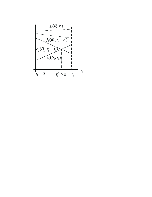
Figure 2: Efficiency Loss in Asymmetric Case

V Conclusion

This work investigated the impact of incomplete information on incentives for node cooperation in parallel relay networks. We considered two situations in which source either has partial bargaining power or full bargaining power. For the situation where the source has partial bargaining power, we have shown that all Nash Equilibria in the complete information game are efficient, including those induced by linear charging functions. We then characterized the Bayesian Nash Equilibrium for the incomplete information game in which relays propose linear pricing functions, and showed that incomplete information can induce inefficiencies, which are exacerbated by asymmetric prior knowledge on the type distribution. In the situation where the source has full bargaining power, we first showed that in the game with complete information, (Bayesian) Nash equilibria exist and are all efficient. Next, we investigated the game with incomplete information. To deal with the difficulty of characterizing the Bayesian Nash Equilibria in this case, we first showed that if a resource allocation outcome can be realized by a Bayesian Nash equilibrium, then there exists a “truth telling” Bayesian Nash equilibrium that realizes the outcome. We then showed that the set of outcomes for the “truth telling” Bayesian Nash equilibria is included in the set of outcomes for the Nash equilibria for a complete information game, in which the link cost functions are replaced by a specified “virtual cost functions.” Using this approach, we obtained for a symmetric network scenario a bound on the amount of inefficiency which may result from incomplete information.

VI Appendix

Proof of Theorem 34: The first and second-order conditions for (31) are:

$$\left.\frac{dE_{\theta_{-i}}\left\{U_{i}(\theta_{i},f(\widetilde{\theta_{i}},\theta_{-i}))\right\}}{d\widetilde{\theta_{i}}}\right|_{\widetilde{\theta_{i}}=\theta_{i}}=0\text{ \ }$$ (38)

and

$$\left.\frac{d^{2}E_{\theta_{-i}}\left\{U_{i}(\theta_{i},f(\widetilde{\theta_{i}},\theta_{-i}))\right\}}{d\widetilde{\theta_{i}}^{2}}\right|_{\widetilde{\theta_{i}}=\theta_{i}}\leq 0.$$ (39)

The first-order condition is equivalent to

$$\left.E_{\theta_{-i}}\frac{dt_{i}(\widetilde{\theta_{i}},\theta_{-i})}{d\widetilde{\theta_{i}}}\right|_{\widetilde{\theta_{i}}=\theta_{i}}$$ (40)

$$= \left.E_{\theta_{-i}}\left\{\frac{\partial C_{i}(\theta_{i},r_{i}(\widetilde{\theta_{i}},\theta_{-i}))}{\partial r_{i}}\frac{dr_{i}(\widetilde{\theta_{i}},\theta_{-i})}{d\widetilde{\theta_{i}}}\right\}\right|_{\widetilde{\theta_{i}}=\theta_{i}}.$$ (41)

The second-order condition is equivalent to

$$\left.E_{\theta_{-i}}\frac{d^{2}t_{i}(\widetilde{\theta_{i}},\theta_{-i})}{d\widetilde{\theta_{i}}^{2}}\right|_{\widetilde{\theta_{i}}=\theta_{i}}$$

$$\leq E_{\theta_{-i}}\left\{\frac{\partial^{2}C_{i}(\theta_{i},r_{i}(\widetilde{\theta_{i}},\theta_{-i}))}{\partial r_{i}^{2}}\left[\frac{dr_{i}(\widetilde{\theta_{i}},\theta_{-i})}{d\widetilde{\theta_{i}}}\right]^{2}\right.$$

$$+\left.\left.\frac{\partial C_{i}(\theta_{i},r_{i}(\widetilde{\theta_{i}},\theta_{-i}))}{\partial r_{i}}\frac{d^{2}r_{i}(\widetilde{\theta_{i}},\theta_{-i})}{d\widetilde{\theta_{i}}^{2}}\right\}\right|_{\widetilde{\theta_{i}}=\theta_{i}}.$$

By evaluating the first-order condition at $\theta_{i}$ differentiating with respect to $\theta_{i}$, we get:

$$E_{\theta_{-i}}\left\{\frac{d^{2}\left\{t_{i}(\theta_{i},\theta_{-i})\right\}}{d\theta_{i}^{2}}\right\}$$

$$= E_{\theta_{-i}}\left\{\frac{\partial^{2}C_{i}(\theta_{i},r_{i}(\theta_{i},\theta_{-i}))}{\partial r_{i}^{2}}\left[\frac{dr_{i}(\theta_{i},\theta_{-i})}{d\theta_{i}}\right]^{2}\right.$$

$$+\frac{\partial C_{i}(\theta_{i},r_{i}(\theta_{i},\theta_{-i}))}{\partial r_{i}}\frac{d^{2}r_{i}(\theta_{i},\theta_{-i})}{d\theta_{i}^{2}}$$

$$+\left.\frac{\partial^{2}C_{i}(\theta_{i},r_{i}(\theta_{i},\theta_{-i}))}{\partial r_{i}\partial\theta_{i}}\frac{dr_{i}(\theta_{i},\theta_{-i})}{d\theta_{i}}\right\}.$$

Comparing with the second-order condition, we get

$$E_{\theta_{-i}}\frac{\partial^{2}C_{i}(\theta_{i},r_{i}(\theta_{i},\theta_{-i}))}{\partial r_{i}\partial\theta_{i}}\frac{dr_{i}(\theta_{i},\theta_{-i})}{d\theta_{i}}\leq 0.$$ (44)

We have already assumed that

$$\frac{\partial^{2}C_{i}(\theta_{i},r_{i}(\theta_{i},\theta_{-i}))}{\partial r_{i}\partial\theta_{i}}\leq 0\text{ for each }\theta_{-i}.$$ (45)

Notice that when an outcome can be realized by a Bayesian Nash Equilibrium, the following condition must hold:

$$\frac{\partial r_{i}(\theta_{i},\theta_{-i})}{\partial\theta_{i}}\geq 0\text{ given any }\theta_{-i}$$ (46)

Otherwise, the source would allocate a higher rate to a lower type relay, which is not optimal. Notice that by (45) and (46),  (44) automatically holds.

Thus, the following conditions are necessary for the first and second-order conditions to hold.

$$\frac{dE_{\theta_{-i}}\left\{t_{i}(\widetilde{\theta_{i}},\theta_{-i})\right\}}{d\widetilde{\theta_{i}}}$$

$$= \left.E_{\theta_{-i}}\frac{\partial C_{i}(\theta_{i},r_{i}(\widetilde{\theta_{i}},\theta_{-i}))}{\partial r_{i}}\frac{dr_{i}(\widetilde{\theta_{i}},\theta_{-i})}{d\widetilde{\theta_{i}}}\right|_{\widetilde{\theta_{i}}=\theta_{i}}$$

$$\frac{\partial r_{i}(\theta_{i},\theta_{-i})}{\partial\theta_{i}}\geq 0\text{ given any }\theta_{-i}$$

Let $V_{i}(\theta_{i},\theta_{-i})=\max_{{\widetilde{\theta_{i}}}}U_{i}(\theta_{i},r_{i}({\widetilde{\theta_{i}},\theta_{-i}}),t_{i}({\widetilde{\theta_{i}},\theta_{-i}}))$. We use the envelope theorem just as we did in the previous sections:

$$\frac{dE_{\theta_{-i}}V_{i}(\theta_{i},\theta_{-i})}{d\theta_{i}} = \left.\frac{\partial{E_{\theta_{-i}}U_{i}(\theta_{i},r}_{i}{(\widetilde{\theta_{i}},\theta_{-i}),t}_{i}{(\widetilde{\theta_{i}},\theta_{-i})}}{\partial{\theta_{i}}}\right|_{\widetilde{\theta_{i}}=\theta_{i}}$$ (47)

$$= \left.-\frac{\partial{E_{\theta_{-i}}C_{i}(\theta_{i},r_{i}(\widetilde{\theta_{i}},\theta_{-i}))}}{\partial\theta_{i}}\right|_{\widetilde{\theta_{i}}=\theta_{i}}$$

Let $\overline{\theta_{i}}$ and $\underline{\theta_{i}}$ be the upper and lower bounds on relay node i’s type, then

$$E_{\theta_{-i}}V_{i}(\theta_{i},\theta_{-i})$$

$$= E_{\theta_{-i}}V_{i}(\underline{\theta_{i}},\theta_{-i})-\int_{\underline{\theta_{i}}}^{\theta_{i}}\frac{\partial E_{\theta_{-i}}{C_{i}(\theta_{i},r_{i}(\theta_{i},\theta_{-i}))}}{\partial{\theta_{i}}}d\theta_{i}$$

We see from the above equation that, as we already assumed $\frac{\partial{C_{i}(\theta_{i},r_{i})}}{\partial{\theta_{i}}}<0$, the expected utility of relay $i$ is non-decreasing with respect to $\theta_{i}$. Thus, to guarantee that constraints (33) holds, the lowest type must receive non-negative profit. On the other hand, the relay with the lowest type can never receive a positive profit, otherwise the source will reduce its profit by some small amount and still guarantee that the contract is acceptable to all, which contradicts the definition of Bayesian Nash Equilibrium. Thus, the lowest type relay should receive zero profit.

$$E_{\theta_{-i}}V_{i}(\underline{\theta_{i}},\theta_{-i})=0$$ (49)

Plugging in, we get

$$E_{\theta_{-i}}V_{i}(\theta_{i},\theta_{-i})=-\int_{\underline{\theta_{i}}}^{\theta_{i}}\frac{\partial E_{\theta_{-i}}{C_{i}(\theta_{i},r_{i}(\theta_{i},\theta_{-i}))}}{\partial{\theta_{i}}}d\theta_{i}$$ (50)

Suppose the type distribution function of relay $i$ is $F_{i}(\theta_{i})$ and the density is $f_{i}(\theta_{i})$. Let $R$ be the expected revenue of the source node. Then,

$$R = E_{\theta}\left\{W_{s}(r_{s})-C_{s}(\theta_{s},r_{0})-\sum_{i}t_{i}(\theta)\right\}$$

$$= E_{\theta}\left\{W_{s}(r_{s})-C_{s}(\theta_{s},r_{0})-\sum_{i}V_{i}(\theta)-\sum_{i}C_{i}(\theta)\right\}$$

$$= E_{\theta}\left\{W_{s}(r_{s})-C_{s}(\theta_{s},r_{0})-\sum_{i}C_{i}(\theta)\right\}$$

$$+\sum_{i}\int_{\underline{\theta_{i}}}^{\overline{\theta_{i}}}f_{i}(\theta_{i})E_{\theta_{-i}}\left[\int_{\underline{\theta_{i}}}^{\theta_{i}}\frac{\partial C_{i}(\theta_{i}^{\prime},r_{i}(\theta_{i}^{\prime},\theta_{-i}))}{\partial\theta_{i}^{\prime}}d\theta_{i}^{\prime}\right]d\theta_{i}$$

$$= E_{\theta}\left\{W_{s}(r_{s})-C_{s}(\theta_{s},r_{0})-\sum_{i}C_{i}(\theta)\right\}$$

$$-\sum_{i}\int_{\underline{\theta_{i}}}^{\overline{\theta_{i}}}E_{\theta_{-i}}\left[\int_{\underline{\theta_{i}}}^{\theta_{i}}\frac{\partial C_{i}(\theta_{i}^{\prime},r_{i}(\theta_{i}^{\prime},\theta_{-i}))}{\partial\theta_{i}^{\prime}}d\theta_{i}^{\prime}\right]$$

$$\times d(1-F_{i}(\theta_{i}))$$

$$= E_{\theta}\left\{W_{s}(r_{s})-C_{s}(\theta_{s},r_{s})-\sum_{i}C_{i}(\theta)\right\}$$

$$-\sum_{i}E_{\theta_{-i}}\left[\int_{\underline{\theta_{i}}}^{\theta_{i}}\frac{\partial C_{i}(\theta_{i}^{\prime},r_{i}(\theta_{i}^{\prime},\theta_{-i}))}{\partial\theta_{i}^{\prime}}d\theta_{i}^{\prime}\right]$$

$$\times(1-F_{i}(\theta_{i}))|_{\underline{\theta_{i}}}^{\overline{\theta_{i}}}$$

$$+\sum_{i}E_{\theta_{-i}}\int_{\underline{\theta_{i}}}^{\overline{\theta_{i}}}(1-F_{i}(\theta_{i}))$$

$$\times d\left[\int_{\underline{\theta_{i}}}^{\theta_{i}}\frac{\partial C_{i}(\theta_{i}^{\prime},r_{i}(\theta_{i}^{\prime},\theta_{-i}))}{\partial\theta_{i}^{\prime}}d\theta_{i}^{\prime}\right]$$

$$= E_{\theta}\left\{W_{s}(r_{s})-C_{s}(\theta_{s},r_{0})-\sum_{i}C_{i}(\theta)\right\}$$

$$+\sum_{i}E_{\theta_{-i}}\int_{\underline{\theta_{i}}}^{\overline{\theta_{i}}}(1-F_{i}(\theta_{i}))$$

$$\times d\left[\int_{\underline{\theta_{i}}}^{\theta_{i}}\frac{\partial C_{i}(\theta_{i}^{\prime},r_{i}(\theta_{i}^{\prime},\theta_{-i}))}{\partial\theta_{i}^{\prime}}d\theta_{i}^{\prime}\right]$$

$$= E_{\theta}\{W_{s}(r_{s})-C_{s}(\theta_{s},r_{0})\}$$

$$-\sum_{i}E_{\theta_{-i}}\int_{\underline{\theta_{i}}}^{\overline{\theta_{i}}}C_{i}(\theta_{i},r_{i}(\theta_{i},\theta_{-i}))$$

$$-\frac{1-F_{i}(\theta_{i})}{f_{i}(\theta_{i})}\frac{\partial C_{i}(\theta_{i},r_{i}(\theta))}{\partial\theta_{i}}f_{i}(\theta_{i})d\theta_{i}$$

$$= E_{\theta}[W_{s}(r_{s})-C_{s}(\theta_{s},r_{0})]$$

$$-E_{\theta}\sum_{i}\left(C_{i}(\theta_{i},r_{i}(\theta))-\frac{1-F_{i}(\theta_{i})}{f_{i}(\theta_{i})}\frac{\partial C_{i}(\theta_{i},r_{i}(\theta))}{\partial\theta_{i}}\right)$$

Thus, we obtain a game with complete information and full source bargaining power where the revenue function is changed to $J_{i}(\theta_{i},r_{i})$ rather than $C_{i}(\theta_{i},r_{i})$.

References

- [1] A. Blanc, Y. Liu, and A. Vahdat, “Designing incentives for peer-to-peer routing,” in Proceedings of IEEE INFOCOM 2005, vol. 1, Mar. 2005.
- [2] J. Crowcroft, R. Gibbens, F. Kelly, and S. Östring, “Modelling incentives for collaboration in mobile ad hoc networks,” Performance Evaluation, vol. 57, no. 4, pp. 427–439, 2004.
- [3] P. Marbach and Y. Qiu, “Cooperation in wireless ad hoc networks: a market-based approach,” IEEE/ACM Transactions on Networking, vol. 13, pp. 1325–1338, Dec. 2005.
- [4] L. Buttyan and J.-P. Hubaux, Security and Cooperation in Wireless Networks. Cambridge University Press, 2007.
- [5] F. Kelly, A. Maulloo, and D. Tan, “Rate control in communication networks: shadow prices, proportional fairness and stability,” Journal of the Operational Research Society, vol. 49, 1998.
- [6] R. Cole, Y. Dodis, and T. Roughgarden, “Pricing network edges for heterogeneous selfish users.,” in Proceedings of the 35th Annual ACM Symposium on Theory of Computing, pp. 521–530, Jun. 2003.
- [7] T. Roughgarden and E. Tardos, “How bad is selfish routing?,” in Proceedings of the 41st Annual Symposium on Foundations of Computer Science, 2000.
- [8] T. Roughgarden, “Selfish routing with atomic players,” in Proceedings of the sixteenth annual ACM-SIAM symposium on Discrete algorithms, pp. 1184–1185, 2005.
- [9] L. He and J. Walrand, “Pricing and revenue sharing strategies for internet service providers,” in Proceedings of the 24th Annual Joint Conference of the IEEE Computer and Communications Societies., vol. 1, pp. 205 – 216 vol. 1, 2005.
- [10] S. Shakkottai and R. Srikant, “Economics of network pricing with multiple isps,” IEEE/ACM Transactions on Networking, vol. 14, no. 6, pp. 1233 –1245, 2006.
- [11] D. Acemoglu and A. Ozdaglar, “Competition and efficiency in congested markets,” Math. Oper. Res., vol. 32, no. 1, pp. 1–31, 2007.
- [12] M. Neely, “Optimal pricing in a free market wireless network,” in INFOCOM 2007. 26th IEEE International Conference on Computer Communications. IEEE, pp. 213 –221, May 2007.
- [13] S. Zhong, J. Chen, and Y. Yang, “Sprite: a simple, cheat-proof, credit-based system for mobile ad-hoc networks,” in Proceedings of IEEE INFOCOM, vol. 3, pp. 1987 – 1997 vol.3, Mar. 2003.
- [14] O. Ileri, S.-C. Mau, and N. Mandayam, “Pricing for enabling forwarding in self-configuring ad hoc networks,” IEEE Journal on Selected Areas in Communications, vol. 23, no. 1, pp. 151 – 162, 2005.
- [15] S. Chawla, F. Niu, and T. Roughgarden, “Bertrand competition in networks,” SIGecom Exch., vol. 8, no. 1, pp. 1–4, 2009.
- [16] Y. Xi and E. Yeh, “Pricing, competition, and routing for selfish and strategic nodes in multi-hop relay networks,” in Proceedings of the 27th Annual Joint Conference of the IEEE Computer and Communications Societies, pp. 1463 –1471, 2008.
- [17] B. Wang, Z. Han, and K. R. Liu, “Distributed relay selection and power control for multiuser cooperative communication networks using stackelberg game,” IEEE Transactions on Mobile Computing, vol. 8, no. 7, pp. 975–990, 2009.
- [18] A. Ozdaglar and R. Srikant, “Incentives and pricing in communication networks,” Algorithmic Game Theory, Cambridge Press, 2007.
- [19] D. P. Bertsekas and R. Gallager, Data Networks. Prentice Hall, second ed., 1992.
- [20] N. Nisan and A. Ronen, “Algorithmic mechanism design (extended abstract),” in Proceedings of the thirty-first annual ACM symposium on Theory of computing, STOC ’99, (New York, NY, USA), pp. 129–140, ACM, 1999.
- [21] P. C. Archer, A. and K. Talwar, “An approximate truthful mechanism for combinatorial auctions with single parameter agents,” Internet Mathematics, vol. 1, no. 2, pp. 129–150, 2006.
- [22] I. Dobson, B. Carreras, V. Lynch, and D. Newman, “Communication requirements of vcg-like mechanisms in convex environments,” in Proceedings of the Allerton Conference on Communication, Control, and Computing, 2005.
- [23] M. Gairing, B. Monien, and K. Tiemann, “Selfish routing with incomplete information,” Theory of Computing Systems, vol. 42, pp. 91–130, 2008. 10.1007/s00224-007-9015-8.
- [24] B. Lebrun, “First price auctions in the asymmetric n bidder case,” International Economic Review, vol. 40, no. 1, pp. pp. 125–142, 1999.