Cluster Turbulence: Simulation Insights

Abstract

Cluster media are dynamical, not static; observational evidence suggests they are turbulent. High-resolution simulations of the intracluster media (ICMs) and of idealized, similar media help us understand the complex physics and astrophysics involved. We present a brief overview of the physics behind ICM turbulence and outline the processes that control its development. High-resolution, compressible, isothermal MHD simulations are used to illustrate important dynamical properties of turbulence that develops in media with initially very weak magnetic fields. The simulations follow the growth of magnetic fields and reproduce the characteristics of turbulence. These results are also compared with full cluster simulations that have examined the properties of ICM turbulence.

1 Introduction

Observation and theory have revealed intracluster media (ICMs) to be very dynamic environments with active “weather” driven by a host of activities such as mergers, accretion, AGNs, galactic winds and instabilities. These drivers are common and cause the ICMs to be criss-crossed by large-scaled, complex flows that generate shocks, contact discontinuities (aka “cold fronts”) and bulk shear. Inevitably such flows should lead to turbulence in the ICMs, an outcome supported by growing observational evidence. These include, for example, substantial ICM random velocities in Perseus reducing resonance scattering in the 6.7 keV iron line [Churazov etal 2004], evidence for thermal ICM pressure fluctuations in the Coma cluster [Shuecker etal 2004], patchy Faraday rotation measure distributions in several clusters [Bonafede etal 2010] and the absence of large scale polarization in cluster radio halos [Kim etal 1990], suggesting disordered magnetic fields.

Turbulence in clusters is important to understand for many reasons. Turbulent pressure helps support the ICM, so relevant cluster mass measures. Turbulence transports entropy, metals and cosmic rays, all important cluster diagnostics. It transports and amplifies magnetic fields, which in turn control ICM viscosity, resistivity and thermal conductivity, as well as the propagation and acceleration of cosmic rays. The literature on turbulence is extensive including excellent reviews on MHD turbulence, which is most relevant to the ICM (e.g., [Brandenburg & Subramanian 2005]). Here we make a few observations pertinent to this meeting.

2 Origins of Cluster Turbulence

Turbulence describes motions possessing significant random velocities. This random velocity can include both compressible ($\nabla\cdot\vec{u}\neq 0$) and vortical, or solenoidal ($\vec{\omega}=\nabla\times\vec{u}\neq 0$) components. In ICM circumstances, which usually involve mostly subsonic flows, the vortical component ordinarily dominates. Thus, understanding this turbulence begins with an identification of the sources of vorticity and the manner in which vorticity evolves.

Euler’s equation for an ideal fluid can be expressed in terms of vorticity [Landau & Lifshitz 1987],

$$\frac{\partial\vec{\omega}}{\partial t}=\nabla\times(\vec{u}\times\vec{\omega})+\frac{1}{\rho^{2}}\nabla\rho\times\nabla P.$$ (1)

This can be rewritten as a conservation law for the integrated vorticity through a surface element moving with the fluid, or by way of Stokes’ Theorem a conservation of circulation around that surface element,

$$\frac{d}{dt}\int\vec{\omega}\cdot d\vec{a}=\frac{d}{dt}\oint\vec{u}\cdot d\vec{l}=\int\frac{1}{\rho^{2}}(\nabla\rho\times\nabla P)\cdot d\vec{a},$$ (2)

where $d/dt$ is the Lagrangian time derivative.

Equation 2 shows that in ideal, barotropic flows, where the pressure depends only on density ($\nabla\rho\times\nabla P=0$), a fluid element’s net vorticity is conserved. Local values of $\vec{\omega}$ still change, of course, without vorticity source terms. For instance, when an incompressible flow element’s cross section is decreased as it is stretched, $\vec{\omega}$ will increase. This vortex stretching (how tornados form) is central to evolution of turbulent flows.

These vorticity properties are analogous to magnetic flux conservation familiar to all astrophysicists. In fact, the magnetic induction equation in ideal MHD is the same as the barotropic form of equation 1 with the substitution $\vec{\omega}\rightarrow\vec{B}$. The vortex stretching analogy applied to magnetic fields means that stretched magnetic flux tubes enhance local fields. The local B of an incompressible flux tube varies in proportion to the length of the tube. Flux tube stretching is, in fact, at the core of the turbulence dynamo, or small scale dynamo that amplifies weak magnetic fields inside turbulent conducting media. Vortical turbulent motions statistically extend the length of a fluid element over time, causing both vorticity and magnetic field to be locally enhanced while conserving total circulation and magnetic flux in an ideal fluid. The root-mean-square (RMS) values of both vorticity and magnetic field intensity grow in this way, even in the absence of source terms.

On the other hand, vorticity can be generated at the curved surface of shocks in and around clusters (e.g., [Ryu etal 2003, Kang etal 2007, Vazza etal 2009]) and by the baroclinity of flows. For uniform upstream flow, the vorticity behind a curved shock surface is

$${\vec{\omega}}_{\rm cs}=\frac{(\rho_{2}-\rho_{1})^{2}}{\rho_{1}\rho_{2}}K{\vec{U}}_{1}\times{\hat{n}},$$ (3)

with $\rho_{1}$ and $\rho_{2}$ the upstream and downstream gas densities, ${\vec{U}}_{1}$ the upstream flow velocity in the shock rest frame, $K$ the shock surface curvature tensor, and ${\hat{n}}$ the shock normal unit vector. If isopycnic (constant density) and isobaric surfaces are not coincident, vorticity is generated according to equation 2. If we let $P=S\rho^{\gamma}$, where $S$ is a proxy for entropy in a $\gamma$-law gas, we see that the baroclinity is introduced by shock induced entropy variations. See [Ryu etal 2008] for more discussion of this issue. AGNs and galactic winds also add shear to ICMs, so equivalently, vorticity ($\omega\sim\Delta u/\delta$, where $\delta$ is the thickness of the shear layer).

Subsequently, the energy in the vortical flows cascades down to smaller scales and turbulence develops, provided the viscous dissipation scale, $l_{visc}$, is smaller than the “driving scale”, $L_{d}$, for the flow. The driving scale, $L_{d}$, is generally comparable to such things as the curvature radius of a shock, the size of a substructure core, or the scale of an AGN or galactic outflow. These likely range from $\sim 10\rm{s}$ of kpc to $\sim 100\rm{s}$ of kpc.

The appropriate viscous dissipation scales in ICMs remain uncertain. The media are hot and very diffuse plasmas, so Coulomb collisions are ineffective. The associated mean free path, $\lambda_{Coul}\sim 1~{}\rm{kpc}~{}T_{keV}^{5/2}/(n_{-3}u_{th,100})$, ranges from $\sim 10$s of pc to $\sim 10$s of kpc, depending on the cluster circumstances. Here $T_{keV}$ is the ICM temperature in keV, $n_{-3}$ is the density in $10^{-3}\rm{cm}^{-3}$ and $u_{th,100}$ is the thermal velocity of ions in $100~{}\rm{km/sec}$. The corresponding kinetic viscosity, $\nu\sim u_{th}\lambda_{Coul}$, is very large, and the Reynolds number, $Re\sim L_{d}U/\nu\sim\rm{few~{}}\times 10$ , with $U\sim u_{th}\sim\rm{few~{}to~{}}10s$, the velocity at the driving scale. Hence, the viscous dissipation scale due to Coulomb scattering alone, $l_{visc}\sim L_{d}/Re^{3/4}$, would range from fractions of a kpc in cooling cores to several 10s of kpc in hot ICMs. On the other hand, it has been suggested that plasmas threaded with weak magnetic fields, like the ones in the ICMs, are subject to gyro-scale instabilities, such firehose and mirror instabilities; then, the scattering of particles with the resulting fluctuations could reduce the particle mean-free path, so also the viscous dissipation scale ([Schekochihin & Cowley 2006]). The detailed picture is still very uncertain. Nevertheless, in our discussion below we assume the physical dissipation scale is at least as small as the effective dissipation scales of the simulations, so of order the grid resolution. In our simulations, the grid resolution would be $\sim 1$ kpc or so (see §3), while for full cluster simulations it is at least several kpc.

The resistive dissipation scales, $l_{res}$, in the ICMs are also uncertain. In a turbulent flow with $\eta\ll\nu$, it is $l_{res}\sim L_{d}/Rm^{1/2}$, where $Rm\sim L_{d}U/\eta$ is the magnetic Reynolds number, and $\eta$ is the resistivity. It is likely that the magnetic Prandtl number $P_{r,M}\equiv Rm/Re=\nu/\eta\ga 1$ in the ICMs. For instance, viscosity and resistivity due exclusively to Coulomb scattering would lead to $P_{r,M}\gg 1$ (e.g., [Spitzer 1978]). In the simulations reported here, both the viscosity and resistivity have numerical origins with dissipation scales of order the grid resolution; thus, $P_{r,M}\sim 1$. Most simulations, including most full cluster simulations, effectively have $P_{r,M}\sim 1$ too. Strictly speaking, the simulations with $P_{r,M}\sim 1$ should be valid only in, and so applied only to the scales of $l\ga l_{visc}$ and $l\ga l_{res}$. For the scales of $l_{res}\la l\la l_{visc}$, simulations with large Prandtl number are required. It is, however, hard to reproduce large Prandtl number turbulence with sufficient viscous and resistive inertial ranges (e.g., [Schekochihin etal 2004]).

3 Simulation of ICM-like Turbulence

It is not simple to isolate turbulence from generally complex motions in real or simulated clusters. As a complementary exercise we have initiated a high-resolution simulation study of the evolution and saturation of driven MHD turbulence in periodic computational domains that resemble ICMs. Since cluster media, while clearly magnetized, are not energetically dominated by magnetic fields, we focus on turbulence developed with initially very weak magnetic fields. The full study considers both compressible and incompressible fluids and ideal and nonideal media with a range of magnetic Prandtl numbers. We report here some initial results of simulations of ideal, compressible MHD turbulence in isothermal media. The simulations used an isothermal ideal MHD code, which is a version updated from that of [Kim etal 2001] for massive parallelization. Results here are from simulations with $1024^{3}$ and $2048^{3}$ grid zones (with the typical cluster sizes $\sim 1$ Mpc, the grid resolution would be $\sim 1$ kpc). The two simulations are very consistent; the higher resolution calculation produces slightly stronger magnetic fields at saturation.

Initially the medium has uniform density, $\rho=1$, with gas pressure, $P=1$, so that the sound speed, $c_{s}=1$. The initially magnetic field is uniform and very weak, with $\beta=P/P_{B}=10^{6}$. The cubic box has dimensions, $L_{0}=L_{x}=L_{y}=L_{z}=10$ with periodic boundaries. Turbulence is driven by solenoidal velocity forcing, drawn from a Gaussian random field determined with a power spectrum $P_{k}\propto k^{6}\exp(-8k/k_{peak})$, where $k_{peak}=2k_{0}$ $(k_{0}=2\pi/L_{0})$, and added at every $\Delta t=0.01L/c_{s}$. The power spectrum peaks around $k_{d}\approx 1.5k_{0}$, or around a scale, $L_{d}\approx 2/3L_{0}$. The amplitude of the perturbations is tuned so that $u_{RMS}\sim 0.5$ or $M_{s}\equiv u_{RMS}/c_{s}\sim 0.5$ at saturation, close to what resuilts in full cluster simulations (e.g., [Nagai etal 2007, Ryu etal 2008, Vazza etal 2009], and see also §4).

Our setup gives a characteristic time scale, $t_{d}=L_{d}/u_{RMS}\approx 15$. In that time the largest eddies should spawn something resembling turbulent behavior. Indeed Fig. 1 shows that the mean turbulent kinetic energy density, $E_{K}$, grows and peaks at $t\sim t_{d}$, with a value corresponding to $u_{RMS}\sim 2/3$. Subsequently, $E_{K}$ slowly declines as the mean magnetic energy density, $E_{B}$ grows. The kinetic energy power spectrum, $E_{K}(k)$, at $t=20$ also shown in Fig. 1, exhibits a peak at $k/k_{0}\sim 2$, near the driving scale, and takes a Kolmogorov-like, inertial form, $E(k)\propto k^{-5/3}$, for $k/k_{0}\la 50$. By this time energy has cascaded from the driving scales far enough that the motions, with negligible magnetic backreaction, are reasonably described as classical, hydrodynamical turbulence over a modest range of scales.

Figure 1: Top: Evolution of kinetic, $E_{K}$, and magnetic, $E_{B}$, energies in simulations of ideal, compressible MHD turbulence for two grid resolutions. Bottom: Power spectra, $E(k)$, of kinetic and magnetic energies at $t=20$ and $t=130$ in the $2048^{3}$ zone turbulence.

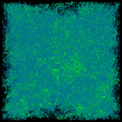
Figure 2: Magnetic energy density distributions in MHD turbulence. Top: Log($E_{B}$) at $t=20$ in $2048^{3}$ simulation. Bottom: Log($E_{B}$) at $t=130$. Higher tones at the late time reflect stronger fields.

Turbulent fluid motions stretch and intensify vorticity and magnetic flux, leading to development of a chaotic sea of vortex and magnetic filaments. This is illustrated for the magnetic field at $t=20$ in the top of Fig. 2. The magnetic filaments in this image have characteristic lengths of a few % of $L_{0}$. This agrees with the fact that the magnetic power spectrum, $E_{B}(k)$, peaks for $k_{peak}/k_{0}\sim 50$ at this time. The transverse dimensions of the filaments, an order of magnitude smaller at this time, seem to correspond to the dissipation scale.

As the magnetic field intensifies, both vorticity and magnetic energies undergo inverse cascades from small to large scales, with the coherence lengths of their filaments growing accordingly. This is evident for the magnetic field in the power spectrum changes in Fig. 1. The inverse cascade of magnetic energy can be understood as follows. The field is wrapped more quickly around smaller scale eddies, because the eddy turn over time varies as $t_{l}\propto l^{2/3}$. Maxwell stresses, $\propto(\nabla\times B)\times B$, then, feed back on the kinetic turbulence, causing significant modifications in the fluid motions, thus saturating the magnetic field growth on a given scale, $l$, when $E_{B}(l)\sim E_{K}(l)$. Since the turbulent kinetic energy on a scale $E_{K}(l)\propto l^{2/3}$, the saturation scale of the magnetic turbulence should evolve over time as $l_{B}\propto t^{3/2}$, while the magnetic energy grows linearly with time, both consistent with Fig. 1. Eventually, as $l_{B}$ approaches the outer scale of the kinetic turbulence, $L_{d}$, the scalings break down and turbulence reaches saturation where the ratio of the total magnetic to kinetic energy is $E_{B}/E_{K}\sim 2/3$ (see also, e.g., [Schekochihin etal 2004, Ryu etal 2008, Cho etal 2009, Cho & Ryu 2009]).

Finally, we emphasize an interesting topological transformation in the flow structure as turbulence proceeds through the linear growth to the saturation stage. Fig. 2 displays the different topologies of the magnetic flux structures at $t=20$ and $t=130$. At the earlier time the field is organized into individual filaments. At the later time those filaments have evolved into striated, ribbon-like forms (see also [Schekochihin etal 2004]). Close examination reveals the ribbons to be laminated, with magnetic field and vorticity interleaved through each cross section on scales of the order the dissipation length. In hydrodynamical turbulence such ribbons would be unstable, but the interplay of vorticity and magnetic field seems to stabilize them in MHD turbulence.

The $t=130$ image in Fig. 2 also highlights the important fact that the magnetic field in MHD tubulence is highly intermittent. Relatively strong field ribbons wrap around large shear leaving weak field cavities. Such structures are quite distinct from what one obtains, for example, if they construct a magnetic field distribution out of a Gaussian random variate, even if the outcome is a magnetic field distribution having exactly the same power spectrum, as illustrated very nicely in previous work by [Waelkens etal 2009].

4 Comparison to Cluster Simulations

Recent high-resolution cluster formation simulations have been analyzed for information about properties of ICM turbulence and its evolution. A few of these simulations include MHD e.g., [Donnert etal 2009, Ruszkowski etal 2010, Xu etal 2010]. With or without magnetic fields, an initial challenge is identifying true turbulence in generally complex flows, especially during and after merging activity. Purely solenoidal motions in simulations in a periodic domain can be cleanly isolated using Fourier transforms (e.g., [Ryu etal 2008]). Otherwise some kind of spatial filtering is needed that analyses the motions only up to a maximum scale, such as the core radius of the cluster (e.g., [Dolag etal 2005]). We mention here a few findings of general significance in this context.

Several studies have emphasized turbulence generation from shocks in and around clusters, especially coming from structure formation generally, and merger activity specifically (e.g., [Kang etal 2007, Ryu etal 2008, Vazza etal 2009]). Several studies found that turbulent energy in post-merger ICMs can be comparable to, although somewhat smaller than, the thermal energy; it commonly reaches levels $E_{K}\sim 1/10-1/4~{}E_{T}$ ([Nagai etal 2007, Ryu etal 2008, Vazza etal 2009]), similar to our simulations discussed in §3. Thus, turbulent pressure may impact on hydrostatic equilibrium-based mass estimates. Simulations also suggest that the relative turbulent pressure support is greater towards cluster outskirts (e.g., [Ryu etal 2008, Lau etal 2009]). The turbulence formed in full cluster simulations does not have a sufficiently wide inertial range to evolve a true Kolmogorov power spectrum. Within that limitation, however, the reported kinetic energy power spectra are consistent with expectations. Several studies demonstrated that cluster turbulence can amplify magnetic fields to at least $\mu$Gauss levels (e.g., [Donnert etal 2009, Xu etal 2010]). This amounts to $\sim$a % or so of the thermal pressure and $\sim$10 % or so of the kinetic turbulent pressure. From simulations such as we reported here, the time to reach equipartition ($E_{B}\sim 2/3E_{K}$) from an initially weak field is many driving scale times. It is not surprising that the fields produced in clusters are well below those levels. By the same token the magnetic field power spectra may peak well below the driving scales. The magnetic power spectrum reported from cluster formation simulations using magnetic fields seeded by AGNs in [Xu etal 2010], for example, is consistent with this expectation.

Turbulence decay generally takes several eddy times on the driving scale once the driving ends. In clusters we expect decay times, $\tau_{d}\ga L_{d,100}/\Delta u_{100}$Gyr, where $L_{d,100}$ in 100 kpc. This is consistent with turbulence decay times $\sim$ Gyr reported in cluster formation simulations (e.g., [Paul etal 2010])

5 Conclusions

Processes such as shocks and outflows are likely to drive turbulence in ICMs. The detailed physics is difficult to model analytically, but simulations allow us to explore it in some detail. Magnetic fields are integral ingredients of both the microphysics of ICM transport properties and essential players in the large scale dynamics. Simulations are revealing important insights into the character of the turbulence, including properties of magnetic fields.