Solution of the time-dependent Dirac equation for describing multiphoton ionization of highly-charged hydrogenlike ions

Abstract

A theoretical study of the intense-field multiphoton ionization of hydrogenlike systems is performed by solving the time-dependent Dirac equation within the dipole approximation. It is shown that the velocity-gauge results agree to the ones in length gauge only if the negative-energy states are included in the time propagation. On the other hand, for the considered laser parameters, no significant difference is found in length gauge if the negative-energy states are included or not. Within the adopted dipole approximation the main relativistic effect is the shift of the ionization potential. A simple scaling procedure is proposed to account for this effect.

I Introduction

Future experiments using an electron-beam ion trap (EBIT) at the Linear Coherent Light Source (LCLS) at Stanford and X-ray Free Electron Laser (XFEL) at Hamburg are expected to permit the study of photoabsorption processes of highly charged atomic ions in the wavelength range of 0.1 to 100 nm with a peak intensity up to $10^{25}$ W/cm² or even higher. Also at the GSI (Darmstadt) experimental investigations of highly charged ions exposed to intense laser fields are planned within the SPARC project. The analysis of these experiments will require a relativistic treatment of the ion-laser interaction.

Clearly, a full treatment demands to solve the time-dependent Dirac equation (TDDE) incorporating also the spatial dependence of the vector potential. Since such a treatment is very demanding, most earlier treatments adopted simplifications. Low-dimensional models are especially popular. Starting first with a one-dimensional treatment Kylstra et al. (1997), elaborate two-dimensional calculations have been reported, e. g., in Rathe et al. (1997); Mocken and Keitel (2004, 2008). However, such models can certainly not provide quantitative predictions and it is, at least a priori, not even clear whether they are always qualitatively correct. Similarly to the non-relativistic case, also simplified ionization models like the strong-field approximation Reiss (1990); Faisal and Bhattacharyya (2004); Klaiber et al. (2006); Faisal (2009), semiclassical tunneling theory Milosevic et al. (2002), or classical models like in Keitel and Knight (1995); Gaier and Keitel (2002); Hetzheim and Keitel (2009) have been proposed. However, in order to allow for quantitative predictions or the validation of such simplified models a full-dimensional solution of the TDDE is needed.

Very recently, a three-dimensional solution of the TDDE for hydrogenlike systems has been reported in Selstø et al. (2009). The radial solutions were expanded on a grid and the TDDE was either solved by a direct propagation on the grid or using a spectral expansion in field-free eigenstates. The spatial dependence of the vector potential of the carrier part of the laser pulse was also considered, while the one in the envelope was ignored. The velocity gauge was used and the importance of including the negative-energy (NE) states was emphasized in the case of a treatment beyond the dipole approximation, even for the considered laser parameters where the photon energy is insufficient to produce real positron-electron pairs. Based on general theoretical considerations it was conjectured that in length gauge the importance of the NE states may be reduced. On the other hand, it was concluded on the basis of the numerical results that within the dipole approximation the inclusion of NE states is not needed, even if the TDDE is solved in velocity gauge. A comparison of the numerically obtained ionization rates for various nuclear charges with the ones in non-relativistic approximation showed that, expectedly, increasing differences are found with increasing charge. However, it was concluded that the ionization rate (shown as a function of the peak value of the laser field) obtained within the relativistic TDDE calculation may be larger or smaller than the non-relativistic result. The authors found the higher rate easier to understand and could only speculate on possible reasons for the lower one.

A solution of the TDDE within the length gauge was reported more recently in Pindzola et al. (2010). A direct time propagation on a grid was used. As in Selstø et al. (2009) the electron-nucleus interaction is described by the unmodified non-relativistic Coulomb interaction. While solely the dipole approximation is adopted, not only results for one-electron, but also for two-electron ions are reported. In the latter case the electron-electron interaction is also described by the non-relativistic Coulomb interaction. No explicit discussion of the inclusion or omission of the NE states is given. Comparing for Ne⁹⁺, Ne⁸⁺, U⁹¹⁺, and U⁹⁰⁺ the photoionization cross sections obtained by solving the TDDE for 10-cycle pulses (using a single pulse with one set of laser parameters for every ion) with the ones of relativistic perturbation theory, a good quantitative agreement is found. This result is, of course, expected, if the laser parameters are chosen in a way that perturbation theory is applicable, as was the case in Pindzola et al. (2010) where relatively low intensities (in relation to the ionization potentials and photon frequencies) were considered.

In this work a further approach for solving the TDDE is presented. It is based on the spectral expansion in field-free eigenstates where the radial wavefunctions are expressed in a $B$-spline basis. It may be seen as an extension of the corresponding approaches for solving the non-relativistic time-dependent Schrödinger equation (TDSE) for one- and two-electron atoms in, e. g., Tang et al. (1990a, b); Lambropoulos et al. (1998); Nubbemeyer et al. (2008), for molecular hydrogen Awasthi et al. (2005); Palacios et al. (2006); Vanne and Saenz (2009); Sansone et al. (2010); Vanne and Saenz (2010), and for in principle arbitrary molecules within the single-active-electron approximation Awasthi et al. (2008); Petretti et al. (2010). While Selstø et al. (2009) and Pindzola et al. (2010) considered mostly (or solely) one-photon ionization, an extension to multiphoton ionization is presented. Clearly, such calculations are very demanding as they require larger expansions, because more angular momenta are involved. Within the dipole approximation a systematic investigation of the importance of NE states as well as the convergence behavior within either length or velocity gauge is performed. A simple scaling relation is proposed that allows to relate relativistic TDDE solutions to the ones obtained with the non-relativistic TDSE, if both are performed within the dipole approximation.

In this work atomic units ($e=m_{e}=\hbar=1$) are used unless specified otherwise.

II Theory

The dynamics of a highly charged atomic ion exposed to an external electromagnetic field is considered by means of both a relativistic and a non-relativistic treatment within the dipole approximation. The vector potential $\mathrm{\mathbf{A}}(t)$ is chosen in the form of an $N$-cycle $\cos^{2}$-shaped laser pulse that is linear-polarized along the $z$ axis,

$$\mathrm{\mathbf{A}}(t)=\begin{cases}\displaystyle\mathrm{\mathbf{e}}_{z}A_{0}\cos^{2}\left(\frac{\pi t}{T}\right)\sin(\omega t),&t\in(-\frac{T}{2},\frac{T}{2});\\ \displaystyle 0,&\text{otherwise,}\end{cases}$$ (1)

where $\omega$ is the radiation frequency and $T=2\pi N/\omega$ is the pulse duration. Ignoring finite nuclear size effects, the interaction of an electron with the nucleus may be approximated by the Coulomb potential

$$U(r)=-\frac{Z}{r},$$ (2)

where $Z$ is the nuclear charge. In all calculations presented in this work the hydrogenlike system is initially prepared in its ground state.

II.1 Relativistic calculations

The relativistic dynamics of the quantum system is governed by the TDDE

$$i\frac{\partial\Psi(t)}{\partial t}=\left[H^{\textrm{D}}_{0}+V(t)\right]\Psi(t)$$ (3)

where $H^{\textrm{D}}_{0}$ is the field-free Dirac Hamiltonian $H^{\textrm{D}}_{0}$,

$$H^{\textrm{D}}_{0}=c\,\bm{\alpha}\cdot\mathrm{\mathbf{p}}+c^{2}\beta+U(r),$$ (4)

and the interaction with the electromagnetic field $V(t)$ can be presented within the dipole approximation either in the velocity (V) or length (L) gauge,

$$\begin{split}V^{\textrm{V}}(t)&=c\,\bm{\alpha}\cdot\mathrm{\mathbf{A}}(t)=c\,\alpha_{z}A(t),\\ V^{\textrm{L}}(t)&=\mathrm{\mathbf{r}}\cdot\mathrm{\mathbf{F}}(t)=zF(t).\end{split}$$ (5)

Here, $\beta$ and the components of the vector $\bm{\alpha}$ are the Dirac matrices, $\mathrm{\mathbf{p}}=-i\bm{\nabla}$ is the momentum operator, $c\approx 137$ is the speed of light, and $\mathrm{\mathbf{F}}(t)=-d\mathrm{\mathbf{A}}(t)/dt$ is the electric field.

As is well known (see, e. g., Grant (2007)), the eigenstates of $H^{\textrm{D}}_{0}$ can be presented as four component spinors

$$\Phi_{\kappa m}(\mathrm{\mathbf{r}})=\frac{1}{r}\left(\begin{matrix}P_{\kappa}(r)\,\chi_{\kappa,m}(\hat{\mathrm{\mathbf{r}}})\\ i\,Q_{\kappa}(r)\,\chi_{-\kappa,m}(\hat{\mathrm{\mathbf{r}}})\end{matrix}\right)$$ (6)

where $\chi_{\kappa,m}(\hat{\mathrm{\mathbf{r}}})$ is an $ls$ coupled spherical spinor, $\kappa$ is the relativistic quantum number of angular momentum, related to the orbital and total angular momenta, $l$ and $j$, as

$$\kappa=\begin{cases}-(j+1/2)=-(l+1),&\text{for}\,\,j=l+1/2,\\ \phantom{-(}j+1/2\phantom{)}=\phantom{-}l,&\text{for}\,\,j=l-1/2;\end{cases}$$ (7)

and the radial functions $P_{\kappa}(r)$ and $Q_{\kappa}(r)$ are solutions of the coupled equations

$$\begin{cases}\displaystyle[U(r)+c^{2}-E]P_{\kappa}(r)+c\left[\frac{\kappa}{r}-\frac{d}{dr}\right]Q_{\kappa}(r)=0\\ \displaystyle[U(r)-c^{2}-E]Q_{\kappa}(r)+c\left[\frac{\kappa}{r}+\frac{d}{dr}\right]P_{\kappa}(r)=0.\end{cases}$$ (8)

For two spinor states, $\Phi_{i}$ and $\Phi_{f}$, characterized by the quantum numbers $\{n_{i},\kappa_{i},j_{i},l_{i},m_{i}\}$ and $\{n_{f},\kappa_{f},j_{f},l_{f},m_{f}\}$, respectively, the time-dependent matrix element $V_{fi}(t)=\langle\Phi_{f}|V(t)|\Phi_{i}\rangle$ can be written as

$$V_{fi}(t)=\delta_{m_{f},m_{i}}\,\delta_{|l_{f}-l_{i}|,1}\,W_{fi}\,M_{fi}(t)$$ (9)

where

$$\begin{split}W_{fi}&=(-1)^{j_{f}-m_{f}}(-1)^{j_{i}+1/2}\sqrt{(2j_{f}+1)(2j_{i}+1)}\\ &\times\left(\begin{matrix}j_{f}&1&j_{i}\\ -m_{f}&0&m_{i}\end{matrix}\right)\left(\begin{matrix}j_{f}&1&j_{i}\\ -1/2&0&1/2\end{matrix}\right)\end{split}$$ (10)

and

$$M^{\textrm{L}}_{fi}(t)=F(t)\int dr\,r\,\Bigl{[}P_{i}(r)P_{f}(r)+Q_{i}(r)Q_{f}(r)\Bigr{]},$$ (11)

$$\begin{split}M^{\textrm{V}}_{fi}(t)=-icA(t)\int dr\,&\Bigl{[}(1+\Delta_{fi})P_{i}(r)Q_{f}(r)\\ &-(1-\Delta_{fi})Q_{i}(r)P_{f}(r)\Bigr{]}\end{split}$$ (12)

with $\Delta_{fi}=(-1)^{j_{f}-j_{i}}(\kappa_{f}-\kappa_{i})$.

In order to describe both bound and continuum states, the atom is confined within a spherical box boundary of radius $R$. This leads to the discretization of the continuum spectrum, whereas the bound states remain unmodified, if $R$ is chosen sufficiently large and not too highly excited Rydberg states are considered.

Introducing in a region $[0,R]$ a $B$-spline set consisting of $n+2$ spline functions $B_{i}(r)$ of order $k$, the radial functions $P(r)$ and $Q(r)$ can be expanded in a $B$-spline basis as

$$P(r)=\sum_{i=1}^{n}p_{i}B_{i+1}(r)\quad Q(r)=\sum_{i=1}^{n}q_{i}B_{i+1}(r)$$ (13)

where the first and the last spline are removed from the expansion to ensure the boundary conditions $P(0)=Q(0)=P(R)=Q(R)=0$. Defining the coefficient vector

$$\mathbf{C}=(p_{1},q_{1},p_{2},q_{2},\dots,p_{n},q_{n}),$$ (14)

the system of equations (8) is transformed into a $2n\times 2n$ generalized banded eigenvalue problem which is efficiently solved using LAPACK routine DSBGVX. This procedure yields for every value of $\kappa$ exactly $n$ negative energy solutions and $n$ positive energy solutions.

As has been discussed in literature since the first solution of the time-independent (stationary) Dirac equation using $B$ splines Johnson et al. (1988), there is the problem of the occurrence of spurious states Drake and Goldman (1981) that are non-physical. Different procedures were proposed to avoid this problem Shabaev et al. (2004); Beloy and Derevianko (2008); Grant (2009). While there can be a problem with their identification in the case of many-electron systems, it is the lowest positive energy state for $\kappa>0$ that represents a spurious state in the present case.

II.2 Non-relativistic calculations

The non-relativistic TDSE

$$i\frac{\partial\Psi(t)}{\partial t}=\left[H_{0}+V(t)\right]\Psi(t)$$ (15)

where $H_{0}$ is the non-relativistic field-free Hamiltonian $H_{0}$,

$$H_{0}=\frac{\mathrm{\mathbf{p}}^{2}}{2}+U(r),$$ (16)

and in contrast to the relativistic case, the interaction with the electromagnetic field $V(t)$ is given in the velocity gauge by

$$V^{\textrm{V}}(t)=\mathrm{\mathbf{p}}\cdot\mathrm{\mathbf{A}}(t)=p_{z}A(t).$$ (17)

Similar to the relativistic case, the eigenstates of $H_{0}$, $\Phi_{lm}(\mathrm{\mathbf{r}})=r^{-1}R_{l}(r)Y_{lm}(\hat{\mathrm{\mathbf{r}}})$, are obtained by projecting the radial function $R_{l}(r)$ onto the $B$-spline basis

$$R(r)=\sum_{i=1}^{n}\rho_{i}\,B_{i+1}(r)$$ (18)

and transforming the radial Schrödinger equation into the $n\times n$ generalized banded eigenvalue problem with respect to a coefficient vector

$$\mathbf{C}=(\rho_{1},\rho_{2},\dots,\rho_{n}),$$ (19)

which yields $n$ solutions for every orbital quantum number $l$.

For two states, $\Phi_{i}$ and $\Phi_{f}$, characterized by the quantum numbers $\{n_{i},l_{i},m_{i}\}$ and $\{n_{f},l_{f},m_{f}\}$, respectively, the time-dependent matrix element $V_{fi}(t)=\langle\Phi_{f}|V(t)|\Phi_{i}\rangle$ can also be written in form of Eq. 9, but with

$$\begin{split}W_{fi}&=(-1)^{l_{f}-m_{f}}(-1)^{l_{f}}\sqrt{(2l_{f}+1)(2l_{i}+1)}\\ &\times\left(\begin{matrix}l_{f}&1&l_{i}\\ -m_{f}&0&m_{i}\end{matrix}\right)\left(\begin{matrix}l_{f}&1&l_{i}\\ 0&0&0\end{matrix}\right)\end{split}$$ (20)

and

$$M^{\textrm{L}}_{fi}(t)=F(t)\int dr\,r\,R_{i}(r)R_{f}(r),$$ (21)

$$M^{\textrm{V}}_{fi}(t)=-iA(t)\int dr\,R_{f}(r)\Bigl{[}\frac{l}{r}R_{i}(r)+R^{\prime}_{i}(r)\Bigr{]}.$$ (22)

II.3 Time propagation

Within the spectral approach, the integration of the TDDE (3) and the TDSE (15) is performed by expanding the function $\Psi(t)$ describing the dynamics of the system in the basis of field-free eigenstates $\Phi_{K}$,

$$\Psi(\mathrm{\mathbf{r}},t)=\sum_{K}C_{K}(t)e^{-iE_{K}t}\Phi_{K}(\mathrm{\mathbf{r}})$$ (23)

where the compound index $K$ represents the full set of quantum numbers and the coefficients $C_{K}(t=-T/2)$ are set to zero for all states except for the initial state for which its value is set to 1. Since the quantum number $m$ is conserved for both cases and the ground state is chosen as initial state, the value of $m$ is fixed to $1/2$ for the relativistic case and to $0$ for the non-relativistic case.

Substituting Eq. (23) into Eq. (3) or TDSE (15) the latter ones are reduced to a system of coupled first-order ordinary differential equations,

$$C^{\prime}_{K}(t)=\sum_{K^{\prime}}e^{i(E_{K}-E_{K^{\prime}})t}\,V_{KK^{\prime}}(t)C_{K^{\prime}}(t)\quad,$$ (24)

which is integrated numerically using a variable-order, variable-step Adams solver.

The ionization yield (after the pulse) is then defined as

$$Y_{\rm ion}=\sum_{K}\left|C_{K}(t=T/2)\right|^{2}$$ (25)

where the summation in Eq. (25) is performed over all discretized continuum states. The convergence can be controlled by varying the value of $l_{\textrm{max}}$ (or $j_{\textrm{max}}$) which limits the number of different symmetries involved in the summation (23).

In the case of the TDDE the question of a proper treatment of the spurious states mentioned in Sec.II.1 arises. The success of the spectral approach relies on the completeness of the states included in the summation, at least for a given box size. In fact, already in the case of the non-relativistic Schrödinger equation the use of a finite box leads to the occurrence of non-physical pseudo states (see, e. g., Lambropoulos et al. (1998)). In this case it turned out to be in fact important to include those states in the spectral expansion, since otherwise some relevant part of the Hilbert space is omitted. In order to decide on the proper treatment of the spurious states of the Dirac equation (due to the $B$-spline expansion), a careful check of the relativistic sum rules Drake and Goldman (1981) was performed that also served as a check of the proper implementation of the length and velocity forms of the dipole-operator matrix elements. On this basis it was concluded that the spurious states could be omitted from the basis for solving the TDDE, since the sum rules were fulfilled in this case. The agreement of the TDDE solutions obtained within the length and the velocity gauge discussed below is another indication that the omission of the spurious states is appropriate.

II.4 Computational details and scaling of the TDSE with $Z$

For the sake of consistency, the same $B$-spline basis set is used for both the relativistic and the non-relativistic treatment. Typically, the values $k=9$ and $n=500$ are used to construct an almost linear knot sequence in which the first 40 intervals increase with a geometric progression using $g=1.05$ and all following intervals have the length of the 40th one. Such a choice ensures an accurate numerical description in the vicinity of the nucleus and, at the same time, a sufficient completeness for a description of the discretized continuum Vanne and Saenz (2004). Depending on the nuclear charge $Z$, a box size of $R=(250/Z)\,a_{0}$ is adopted. This choice of $R$ reflects the well-known scaling property of the time-independent Schrödinger equation of hydrogenlike systems. With the substitution $\mathrm{\mathbf{r}}^{\prime}=\mathrm{\mathbf{r}}/Z$ and $E^{\prime}=Z^{2}E$ for the position $\mathrm{\mathbf{r}}$ and the energy $E$, respectively, the eigensolutions for a hydrogenlike system with charge $Z$ reduces to the one of the hydrogen atom with $Z=1$.

Within the dipole approximation this property is preserved also for the TDSE, if the pulse parameters are also properly scaled, e. g., the time as $t^{\prime}=t/Z^{2}$, the laser frequency as $\omega^{\prime}=Z^{2}\omega$, the amplitude of the vector potential as $A_{0}^{\prime}=ZA_{0}$, and the laser peak intensity as $I^{\prime}=Z^{6}I$. Since this property does not persist in case of the relativistic treatment, and the properly scaled solutions of the TDDE are thus not identical anymore, any deviation from the non-relativistic prediction based on the scaling relations can be classified as a relativistic effect, cf. Selstø et al. (2009).

III Results and discussion

III.1 Convergence behavior

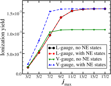
Figure 1: Convergence study with respect to the maximal value of the total angular momentum $j_{\textrm{max}}$. The relativistic calculations of the ionization yield for an ion with the nuclear charge $Z=50$ exposed to a $20$-cycle cos²-shaped laser pulse with peak intensity $I=5\times 10^{23}$W/cm² and a photon energy of $500$ a.u. are performed using the length (L) or velocity (V) gauge either including or excluding the negative energy (NE) states in the expansion (23).

The handling of the NE solutions of the Dirac equation is an important issue and steered considerable attention in the literature, see Fursa and Bray (2008); Selstø et al. (2009) and references therein. The question is whether the NE states should be removed from the basis as long as the creation of real positron-electron pair is energetically out of reach. Such a situation occurs, for example, in case of ionization of an ion with the nuclear charge $Z=50$ exposed to a pulse with photon energy 500 a.u. (see Fig. 1). Whereas only 3 photons are sufficient for ionization, more than 70 photons are required for positron-electron pair creation. As is demonstrated in Fig. 1, the answer to the question of the proper treatment of the NE states depends already within the dipole approximation adopted here clearly on the gauge and thus the interaction operator used in the time propagation. For the length gauge the exclusion of NE states has virtually no effect on the final result. In contrast, for the velocity gauge the results are obviously different. If the NE states are included in the time propagation, the converged result agrees with the one obtained using the length gauge, whereas without the NE states the converged result differs in this example by a factor of about 1.5. Therefore, these states are absolutely necessary for obtaining the correct result.

From the practical point of view the finding is also interesting, since the omission of the NE states and thus half of the total number of states reduces the numerical efforts tremendously. Clearly, doubling the number of states leads to an increase of the number of operations per time step by a factor 4, since the number of transition dipole matrix elements increases by this factor. In the present example (and for a given number of $j_{\textrm{max}}$) the time propagation in length gauge without the NE states is by about a factor of 6 faster compared to the one where the NE states are included. The additional time difference (factor of about 1.5) arises from an increased number of time steps required for convergence in the used adaptive time propagation, if the NE states are included. In fact, the length-gauge time propagation by itself is found to be about 6 times faster than the one performed in velocity gauge, even if the NE states are included in both of them. This factor is due to the finer time grid needed for convergence in velocity gauge. Considering both effects together, even a speed-up by a factor of 50 is found when comparing the length-gauge calculation without NE states and the velocity-gauge variant with NE states that for sufficiently large value of $j_{\textrm{max}}$ both yield practically identical results.

However, Fig. 1 reveals also that the calculations in velocity gauge converge faster with respect to the quantum numbers $j$ included in the calculation. Therefore, the efficiency gain of the length gauge is smaller than the value given above. In the concrete example shown in Fig. 1 the (within better than 0.1 %) converged length-gauge calculation ($j_{\textrm{max}}=15/2$, without NE states) is by a factor of about 40 faster than the (within about 10${}^{-3}\,$%) converged velocity-gauge result ($j_{\textrm{max}}=11/2$, with NE states). Even compared to the only about $0.5\,$% converged velocity-gauge result with $j_{\textrm{max}}=9/2$ (with NE states) there is still a factor of about 30 in time gain. On the other hand, the question of the most efficient choice of the gauge depends on the laser parameters. If few-photon processes, in the most extreme case one-photon ionization at low intensities, are considered, the average angular momentum $j$ transferred to the ion is small. In such a case the need for a larger value of $j_{\textrm{max}}$ in the length-gauge calculation could even overcompensate the gain from the exclusion of the NE states. However, if the average number of absorbed photons increases (due to a smaller ratio of the photon frequency with respect to the ionization potential or due to a higher laser intensity), the relative increase in $j$ due to the slower convergence leads to a smaller increase of the total number of states than the inclusion of the NE states. In this multiphoton regime calculations in length gauge appear to be much more efficient. This finding for the TDDE solution seems to differs from the one for the non-relativistic TDSE where the velocity gauge is often supposed to converge faster than the length gauge.

For extremely high intensities around and above the critical field strength $F_{\rm cr}=c^{3}\approx 2.57\,\times\,10^{6}$ where real pair production is possible, the inclusion of the NE states is, of course, required also in length gauge. In fact, already for the parameters discussed in the context of Fig. 1 we find a relative deviation between otherwise converged length-gauge results with and without NE states of about $2.2\,\times\,10^{-5}$. This appears reasonable, since it is of the order of the (reciprocal) rest energy $c^{-2}\approx 5.3\,\times\,10^{-5}$. For very high laser intensities the gain from omitting the NE states is thus lost and future calculations will have to show whether in that regime length-gauge calculations can still profit from the need of a sparser time grid, or whether the faster convergence with $j$ persists in velocity gauge and may make this gauge more efficient.

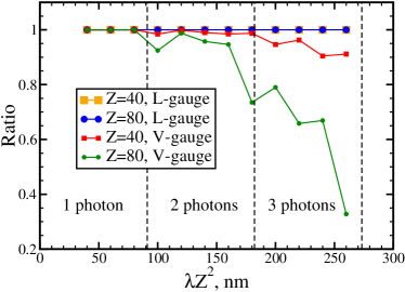
Figure 2: Ratio of the ionization yields that are obtained by either excluding or including the negative energy states in the expansion (23) adopting either length (L) or velocity (V) gauge. The calculations are performed for an ion with two different values of nuclear charge $Z$ by varying the wavelength $\lambda$ of a $20$-cycle cos²-shaped laser pulse with the peak intensity $Z^{6}\times 10^{13}$W/cm². The character of the ionization process changes from single-photon ionization ($\lambda Z^{2}=40\,$nm) to three-photon ionization ($\lambda Z^{2}=260\,$nm).

In Selstø et al. (2009) it was concluded on the basis of the numerical results that the inclusion of the NE states is not crucial for solving the TDDE, if the dipole approximation is adopted. This result was found despite the fact that the calculation was performed in velocity gauge. Therefore, this finding appears to contradict our conclusions. However, it turns out that the importance of the inclusion of the NE states depends in fact on the character of the multiphoton ionization process, i. e. on the number of photons. Figure 2 shows the ratio of the ionization yields obtained either with or without inclusion of the NE states for both gauges and two values of the nuclear charge $Z$. In agreement with the findings discussed above, the inclusion of the NE states has practically no influence for the length-gauge results, independently of the number of photons involved or the nuclear charge. This changes, however, if the velocity gauge is used in the time propagation. The importance of the NE states increases with the order of the multiphoton process (the number of photons required for ionization) and with the nuclear charge. Within the one-photon regime there is practically no influence of the NE states. Thus the finding in Selstø et al. (2009) is confirmed that even in velocity gauge an inclusion of the NE states is not required for calculations in the dipole approximation. However, it is to be understood that those findings apply only to the case where one photon is sufficient to reach into the ionization continuum. Quite remarkable is also the strong dependence of the importance of the NE states on $Z$. For example, for the wavelength $\lambda=260/Z^{2}$ nm the exclusion of the NE states leads to a three times smaller value of the ionization yield for $Z=80$, whereas for $Z=40$ the decrease is only about 10 %. The $Z$ dependence can also explain the negligible effect of NE states within the dipole approximation found in Fig. 1 of Selstø et al. (2009) where $Z=1$ was used. Furthermore, only the probability of remaining in the initial ground state was considered and this quantity is found to converge much faster than, e. g., the ionization yield. This could possibly make it also less sensitive to the NE states.

III.2 Single-photon ionization

As has been discussed in Sec. II.4, the solution of the TDSE for different nuclear charges $Z$ gives identical ionization yields, if the laser pulse parameters are scaled properly. For example, the insert in Fig. 3 shows the non-relativistic ionization yields obtained for an ion with the nuclear charge $Z$ exposed to a $20$-cycle cos²-shaped laser pulse with a peak intensity of $Z^{6}\times 10^{11}$W/cm² for photon energies varying in the range between $15\,Z^{2}\,$eV and $45\,Z^{2}$ eV. Since the ionization potential of the ion is equal to $13.6\,Z^{2}$ eV, the ionization should occur via absorption of a single photon. In order to study the relativistic effects in this one-photon ionization regime, the TDDE is solved for the same system and for 5 different values of $Z$ (in between 40 and 80 with a stepsize of 10).

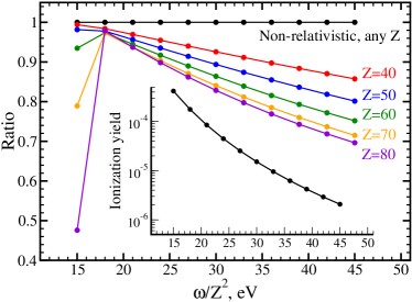
Figure 3: Ratios of the relativistic ionization yields to the non-relativistic ones (shown in the insert) obtained for 5 different values of the nuclear charge $Z$ by varying the carrier frequency $\omega$ of a $20$-cycle cos²-shaped laser pulse with the peak intensity of $Z^{6}\times 10^{11}$W/cm².

The ratio of the relativistic to the non-relativistic ionization yield is shown in Fig. 3. Two features can be observed. First, above $18\,Z^{2}\,$eV the ratio decreases with increasing photon energy. Thus relativistic effects are more pronounced for higher photon frequencies $\omega$. As could be expected, this effect becomes more and more important as $Z$ increases. Second, a discontinuity develops with increasing $Z$ at a photon energy of about $18\,Z^{2}\,$eV. Especially for large values of $Z$ the ratio for the lowest considered photon energy drops down substantially for increasing $Z$. This is a manifestation of the fact that the ionization potential of the ion increases as a consequence of the relativistic velocity of an electron in the vicinity of strong Coulomb potentials. The shift of the ionization potential

$$\Delta I_{p}=I^{\textrm{rel}}_{p}(Z)-I_{p}^{\textrm{nr}}(Z)=c^{2}\left(1-\sqrt{1-\frac{Z^{2}}{c^{2}}}\right)-\frac{Z^{2}}{2}$$ (26)

rapidly increases with increasing $Z$. (For example, $\Delta I_{p}\approx Z^{4}/(8c^{2})$ for small $Z$.) Thus, for $Z=80$ the absorption of a single photon with the energy $15\,Z^{2}$ eV is not sufficient for ionization anymore and the character of the ionization process changes from single-photon to two-photon ionization. For the considered intensities the latter process possesses of course a much smaller probability. In fact, the ratio would be even smaller, if the ratio at $15\,Z^{2}$ eV would correspond to pure two-photon ionization. The finite spectral width of the adopted 20-cycle laser pulse allows, however, one-photon ionization to occur even at this energy and increases thus the ionization yield. Therefore, a finer photon-frequency grid in between $15\,Z^{2}$ eV and $20\,Z^{2}$ eV would show a much smoother behavior than the one visible from Fig. 3.

In Selstø et al. (2009) (Fig. 5) relativistic effects were considered by a comparison of the ionization rates obtained with the TDSE and the TDDE where the latter was solved for 8 different values of $Z$. However, there the behavior was studied as a function of the laser field amplitude (also scaled by the corresponding non-relativistic scaling relations) and for a fixed photon frequency. The authors discuss stabilization, since the ionization rate does not increase monotonously with the field strength, but instead decreases for intensities beyond about $F_{0}=1\,Z^{3}$. The for large values of $Z$ increasing value of $F_{0}$ for which the ionization rate has its maximum is then explained by the stabilization criterion of Gavrila (see Gavrila (2002) and references therein) and the conjecture that due to the lower energy of the ground state in the relativistic case the condition for the occurrence of stabilization shifts to higher field strengths.

In fact, the dependence of the ionization rates on $Z$ discussed in Selstø et al. (2009) may be quantitatively understood from the scaling relations together with the lowering of the ground-state energy due to relativistic effects. This is illustrated in the following way. From the condition $I^{\textrm{rel}}_{p}(Z)=I_{p}^{\textrm{nr}}(Z^{\prime})$ one finds a scaled nuclear charge

$$Z^{\prime}=\sqrt{2c^{2}\left(1-\sqrt{1-Z^{2}/c^{2}}\right)},$$ (27)

for a given true charge $Z$. This allows to estimate the relativistic ionization rate from a non-relativistic calculation using

$$\Gamma^{\prime}(F_{0})=\left(\frac{Z^{\prime}}{Z}\right)^{2}\,\Gamma\left(F_{0}\left[\frac{Z}{Z^{\prime}}\right]^{3}\right)\quad,$$ (28)

if the dependence of the non-relativistic ionization rate on the photon frequency is ignored. In order to obtain non-relativistic ionization rates $\Gamma(F_{0})$, Floquet calculations were performed as a function of the peak amplitude $F_{0}$ of the electric field using program STRFLO Potvliege (1998). They are shown in Fig. 4 and are in reasonable agreement with the TDSE rates in Selstø et al. (2009). Based on the non-relativistic Floquet rates the scaling relation (28) allows to estimate the relativistic rates that are also shown in Fig. 4 for $Z=36$, 54, and 86. The qualitative agreement with the TDDE results in Fig. 5 of Selstø et al. (2009) is satisfactory and especially the shift of the maximum to higher fields is well reproduced. However, in agreement with the discussion in Selstø et al. (2009) the model predicts that the maximum of the ionization rate increases monotonically with $Z$. This is in contrast to the numerical findings in Selstø et al. (2009).

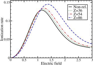
Figure 4: Ionization rate (in units of $Z^{2}$ a.u.) of a hydrogenlike ion exposed to a monochromatic laser field with the frequency $\omega=Z^{2}$ as a function of the amplitude of the electric field (given in units of $Z^{3}$ a.u.) The black solid curve presents the (non-relativistic) Floquet ionization rate, whereas the other curves present the ionization rates obtained using the scaling relation 28 in order to estimate the relativistic ionization rates for three different values of $Z$.

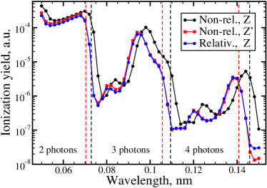
Figure 5: Relativistic (blue circles) and non-relativistic (black circles) ionization yields obtained for an ion with the nuclear charge $Z=50$ exposed to a $20$-cycle cos²-shaped laser pulse with a peak intensity of $5\times 10^{22}$ W/cm² and various laser wavelengths. Additionally, the non-relativistic ionization yields (red squares) for an ion with the nuclear charge $Z^{\prime}=50.88$ are shown whose non-relativistic ionization potential is equal to the relativistic ionization potential of the ion with $Z=50$. The non-relativistic $N$-photon thresholds ($N=2-4$) for $Z$ and $Z^{\prime}$ are indicated by black and red vertical dashed lines, respectively.

III.3 Multiphoton ionization

If many photons are required for ionization, the relativistic results may deviate from the non-relativistic ones by an order of magnitude or more. This is demonstrated in Fig. 5 where relativistic and non-relativistic ionization yields are compared for an ion with the nuclear charge $Z=50$. The laser wavelength varies in the range from 0.05 nm (2-photon ionization) to 0.15 nm (5-photon ionization). Whereas the general structure of the wavelength dependence is similar for both relativistic and non-relativistic treatments, the difference in the positions of all pronounced features like peaks and minima may result in a substantial discrepancy, if the ion yields are compared at a single photon frequency. Obviously, the sharp steps are due to the $N$-photon channel closings and the peaks are signatures of resonantly enhanced multiphoton ionization (REMPI) processes. Their positions are directly related to excitation energies and the ionization potential, respectively, and both are higher in the relativistic than in the non-relativistic case.

In view of the scaling relation (27) it is interesting to compare the TDDE result (for $Z=50$) with the non-relativistic TDSE result for the scaled nuclear charge $Z^{\prime}=50.88$. As can be seen from Fig. 5, the obtained TDSE results deviate from the relativistic ones for $Z=50$ only by a few percent. This indicates that the change of the ionization potential is the by far dominating relativistic effect, at least if multiphoton ionization is described within the dipole approximation. Other possible effects like the splitting of (resonant) intermediate states due to spin-orbit coupling are thus very small, but can be quantified more easily, after the scaling relation has accounted for the main effect. The dominant influence of the shift of the ionization potential is likely to depend on the considered laser intensity and photon frequency. It should be reminded that the Keldysh parameter $\gamma=\sqrt{2\,I_{p}}\omega/F_{0}$ Keldysh (1965) varies in Fig. 5 in between 38.17 and 12.72. This is deep in the multiphoton regime, in fact even in the perturbative one.

IV Conclusion

Single- and multiphoton ionization of highly charged atomic ions has been numerically studied by a direct solution of the time-dependent Dirac equation within the dipole approximation. The stationary Dirac equation is solved by projecting the radial part onto a $B$-spline basis and the obtained field-free eigensolutions are used in the subsequent time propagation. Results for both length and velocity gauges for describing the ion-field interaction are obtained and compared. The inclusion of the negative-energy Dirac states for the description of the relativistic dynamics is shown to be important in the case of the multiphoton ionization, if the velocity gauge is adopted, even if the considered intensities and frequencies are too low for allowing non-negligible real pair creation. If ionization occurs via absorption of a single photon or the time propagation is performed in the length form, the role of negative energy states is much less significant.

Comparing solutions of the time-dependent Dirac and Schrödinger equations for the same ion and laser pulses, the relativistic change of the ionization potential is demonstrated to dominate other relativistic effects in the case of multiphoton ionization. It is shown that this effect is successfully accounted for by a simple scaling relation.

References

- Kylstra et al. (1997) N. J. Kylstra, A. M. Ermolaev, and C. J. Joachain, J. Phys. B 30, L449 (1997).
- Rathe et al. (1997) U. W. Rathe, C. H. Keitel, M. Protopapas, and P. L. Knight, J. Phys. B 30, L531 (1997).
- Mocken and Keitel (2004) G. R. Mocken and C. H. Keitel, J. Comp. Phys. 199, 558 (2004).
- Mocken and Keitel (2008) G. R. Mocken and C. H. Keitel, Comp. Phys. Comm. 178, 868 (2008).
- Reiss (1990) H. R. Reiss, JOSA B 7, 574 (1990).
- Faisal and Bhattacharyya (2004) F. H. M. Faisal and S. Bhattacharyya, Phys. Rev. Lett. 93, 053002 (2004).
- Klaiber et al. (2006) M. Klaiber, K. Z. Hatsagortsyan, and C. H. Keitel, Phys. Rev. A 73, 053411 (2006).
- Faisal (2009) F. H. M. Faisal, J. Phys. B 42, 171003 (2009).
- Milosevic et al. (2002) N. Milosevic, V. P. Krainov, and T. Brabec, J. Phys. B 35, 3515 (2002).
- Keitel and Knight (1995) C. H. Keitel and P. L. Knight, Phys. Rev. A 51, 1420 (1995).
- Gaier and Keitel (2002) L. N. Gaier and C. H. Keitel, Phys. Rev. A 65, 023406 (2002).
- Hetzheim and Keitel (2009) H. G. Hetzheim and C. H. Keitel, Phys. Rev. Lett. 102, 083003 (2009).
- Selstø et al. (2009) S. Selstø, E. Lindroth, and J. Bengtsson, Phys. Rev. A 79, 043418 (2009).
- Pindzola et al. (2010) M. S. Pindzola, J. A. Ludlow, and J. Colgan, Phys. Rev. A 81, 063431 (2010).
- Tang et al. (1990a) X. Tang, H. Rudolph, and P. Lambropoulos, Phys. Rev. Lett. 65, 3269 (1990a).
- Tang et al. (1990b) X. Tang, T. N. Chang, P. Lambropoulos, S. Fournier, and L. F. DiMauro, Phys. Rev. A 41, 5265 (1990b).
- Lambropoulos et al. (1998) P. Lambropoulos, P. Maragakis, and J. Zhang, Phys. Rep. 305, 203 (1998).
- Nubbemeyer et al. (2008) T. Nubbemeyer, K. Gorling, A. Saenz, U. Eichmann, and W. Sandner, Phys. Rev. Lett. 101, 233001 (2008).
- Awasthi et al. (2005) M. Awasthi, Y. V. Vanne, and A. Saenz, J. Phys. B 38, 3973 (2005).
- Palacios et al. (2006) A. Palacios, H. Bachau, and F. Martín, Phys. Rev. Lett. 96, 143001 (2006).
- Vanne and Saenz (2009) Y. V. Vanne and A. Saenz, Phys. Rev. A 80, 053422 (2009).
- Sansone et al. (2010) G. Sansone, F. Kelkensberg, J. F. Perez-Torres, F. Morales, M. F. Kling, W. Siu, O. Ghafur, P. Johnsson, M. Swoboda, E. Benedetti, et al., Nature 465, 763 (2010).
- Vanne and Saenz (2010) Y. V. Vanne and A. Saenz, Phys. Rev. A 82, 011403 (2010).
- Awasthi et al. (2008) M. Awasthi, Y. V. Vanne, A. Saenz, A. Castro, and P. Decleva, Phys. Rev. A 77, 063403 (2008).
- Petretti et al. (2010) S. Petretti, Y. V. Vanne, A. Saenz, A. Castro, and P. Decleva, Phys. Rev. Lett. 104, 223001 (2010).
- Grant (2007) I. Grant, Relativistic Quantum Theory of Atoms and Molecules, vol. 40 of Atomic, Optical, and Plasma Physics (Springer, New York, 2007).
- Johnson et al. (1988) W. R. Johnson, S. A. Blundell, and J. Sapirstein, Phys. Rev. A 37, 307 (1988).
- Drake and Goldman (1981) G. W. F. Drake and S. P. Goldman, Phys. Rev. A 23, 2093 (1981).
- Shabaev et al. (2004) V. M. Shabaev, I. I. Tupitsyn, V. A. Yerokhin, G. Plunien, and G. Soff, Phys. Rev. Lett. 93, 130405 (2004).
- Beloy and Derevianko (2008) K. Beloy and A. Derevianko, Comp. Phys. Comm. 179, 310 (2008).
- Grant (2009) I. P. Grant, J. Phys. B 42, 055002 (2009).
- Vanne and Saenz (2004) Y. V. Vanne and A. Saenz, J. Phys. B 37, 4101 (2004).
- Fursa and Bray (2008) D. V. Fursa and I. Bray, Phys. Rev. Lett. 100, 113201 (2008).
- Gavrila (2002) M. Gavrila, J. Phys. B 35, R147 (2002).
- Potvliege (1998) R. M. Potvliege, Comp. Phys. Comm. 114, 42 (1998).
- Keldysh (1965) L. V. Keldysh, Sov. Phys. JETP 20, 1307 (1965).