Nano-Hertz Gravitational Waves Searches with
Interferometric Pulsar Timing Experiments

Abstract

We estimate the sensitivity to nano-Hertz gravitational waves of pulsar timing experiments in which two highly-stable millisecond pulsars are tracked simultaneously with two neighboring radio telescopes that are referenced to the same time-keeping subsystem (i.e. “the clock”). By taking the difference of the two time-of-arrival residual data streams we can exactly cancel the clock noise in the combined data set, thereby enhancing the sensitivity to gravitational waves. We estimate that, in the band ($10^{-9}-10^{-8}$) Hz, this “interferometric” pulsar timing technique can potentially improve the sensitivity to gravitational radiation by almost two orders of magnitude over that of single-telescopes. Interferometric pulsar timing experiments could be performed with neighboring pairs of antennas of the forthcoming large arraying projects.

The direct detection of gravitational waves is one of the most challenging experimental efforts in physics today. A successful observation will not only represent a great triumph in experimental physics, but will also provide a new observational tool for obtaining a better and deeper understanding about their sources, as well as a unique test of the various proposed relativistic metric theories of gravity Thorne1987 .

Pulsar timing experiments aimed at the detection of gravitational radiation have been performed for decades now. The basic principle underlining the pulsar timing technique is the same as that of other gravitational wave detector designs LIGO ; VIRGO ; GEO ; TAMA ; DOPPLER ; PPA98 : to monitor the frequency variations of a coherent electromagnetic signal exchanged by two or more “point particles” separated in space. As a pulsar continuously emits a series of radio pulses that are received at Earth, a gravitational wave passing across the pulsar-Earth link introduces fluctuations in the time-of-arrival (TOA) of the received electromagnetic pulses. By comparing the pulses TOAs against those predicted by a model, it is in principle possible to detect the effects induced by any time-variable gravitational fields present, such as the transverse-traceless metric curvature of a passing plane gravitational wave train Pulsar . The frequency band in which the pulsar timing technique is most sensitive to ranges from about $10^{-9}$ to $10^{-6}$ Hz, with the lower-limit essentially determined by the overall duration of the experiment ($10^{-9}\ {\rm Hz}\simeq 1/{\rm 30\ years}$), and the upper limit identified by the signal-to-noise ratio of the received radio pulses. To attempt observations of gravitational waves in this way, it is thus necessary to control, monitor and minimize the effects of other sources of timing fluctuations, and, in the data analysis, to use optimal algorithms based on the different characteristics of the pulsar timing response to gravitational waves (the signal) and to the other sources of timing fluctuations (the noise).

A quantitative analysis of the noise sources affecting millisecond pulsar timing searches for gravitational radiation has been highlighted in a recent paper by Jenet et al. JAT2011 . There it has been shown that, in the region ($10^{-9}-10^{-8}$) Hz of the accessible frequency band, the main noises are due to:

1. finiteness of the signal-to-noise ratio in the raw observations;

2. uncertainties in solar system ephemerides, which are used to correct arrival times at the Earth to the barycenter of the solar system;

3. variation of the index of refraction in the interstellar and interplanetary plasma;

4. intrinsic rotational stability of the pulsar, and

5. instability of the local clock against which pulsars are timed, and noise in time transfer if the clock is not located at the observatory site.

Although the timing fluctuations induced by most of these noises can be in principle either reduced or calibrated out, the fundamental noise-limiting sensitivity of pulsar timing experiments is imposed by the timing-fluctuations inherent to the reference clocks that control the TOA measurements. The noise analysis in JAT2011 indicated that clocks such as the Linear-Ion-Trapped-Standard (LITS) (presently in-the-field state-of-the art atomic clocks with long-time-scale timing stability) would result in a sinusoidal strain sensitivity of pulsar timing searches for gravitational waves to a level of about $10^{-15}$ after coherently integrating the data for a period of $10$ years. Since the characteristic wave amplitude associated with a super-massive black-hole-binaries background is predicted to be of comparable magnitude at the frequency $3\times 10^{-9}$ Hz Black1 ; Black2 , it is clear that a single telescope will not be able to unambiguously detect such a gravitational wave signal.

A method for statistically enhancing the signal-to-noise ratio of pulsar timing experiments to backgrounds of gravitational waves was first proposed by Hellings and Downs HD1983 and further analyzed and improved by Jenet et al. JHLM2005 . This technique relies on cross-correlating pairs of TOA residuals data taken by an array of radio telescopes observing highly-stable millisecond pulsars. Since the gravitational wave background is common to all the timing residuals while many noises affecting them are in principle uncorrelated, the cross-correlation technique enhances the strength of the gravitational wave signal over that of the noise.

The experimental configuration we propose in this letter is complementary to the cross-correlation method, in that it provides a way for exactly canceling the clock noise from pairs of TOAs residuals. This is possible by relying on TOAs residuals measured simultaneously by two neighboring radio telescopes tracking, with the same clock, two highly-stable millisecond pulsars located in two different parts of the sky. Since the two TOAs responses to the gravitational wave signal will be different while the clock timing noise transfer function in the two TOA residuals will be the same, by taking the difference of the two time series the clock noise is exactly canceled from the resulting synthesized data while sensitivity to a gravitational wave signal is preserved.

Let us denote with $R_{1}(t)$, $R_{2}(t)$ the two time-of-arrival residuals measured at time $t$ at the two telescopes. Their time derivatives can be written in the following way EW1975 ; Burke1975 ; Wahlquist1987

$$\frac{dR_{i}(t)}{dt} = (1-{\bf{\hat{k}}}\cdot{\bf{\hat{n}}}_{i})\ [\Psi_{i}(t-L_{i}(1+{\bf{\hat{k}}}\cdot{\bf{\hat{n}}}_{i}))-\Psi_{i}(t)]$$ (1)

$$+C(t)+N_{i}(t)\ \ \ \ i=1,2\ ,$$

where we have denoted with $C(t)$ the random process associated with frequency fluctuations due to the clock (common to the two timing residual measurements), with $N_{i}(t)\ ,\ i=1,2$ the two random processes associated with frequency fluctuations due to all other noise sources affecting the timing residuals, and the function $\Psi_{i}(t)$ contains the contribution of a spin-2 gravitational wave transverse-traceless strain tensor ${\bf{h}}$ in the following way

$$\Psi_{i}(t)=\frac{({\bf{\hat{n}}}_{i}\cdot{\bf{h}}\cdot{\bf{\hat{n}}}_{i})}{2[1-({\bf{\hat{k}}}\cdot{\bf{\hat{n}}}_{i})^{2}]}\ .$$ (2)

In Eqs.(1, 2) $\ \ {\bf{\hat{n}}}_{i}L_{i}\ ,\ i=1,2$ is the vector oriented from telescope $i$ to pulsar $i$, ${\bf{\hat{k}}}$ is the unit vector associated with the direction of propagation of the wave, and the symbol $\cdot$ is the operation of scalar product (see Fig. 1). If we denote with $\Delta{\dot{R}}$ the difference of the time-derivative of the two timing residuals given in Eq. (1), we find the resulting interferometric pulsar timing response

$$\Delta{\dot{R}}(t) \equiv {\dot{R}}_{1}(t)-{\dot{R}}_{2}(t)=N_{1}(t)-N_{2}(t)$$ (3)

$$+ [(1-{\bf{\hat{k}}}\cdot{\bf{\hat{n}}}_{2})\ \Psi_{2}(t)-(1-{\bf{\hat{k}}}\cdot{\bf{\hat{n}}}_{1})\ \Psi_{1}(t)]$$

$$+ [(1-{\bf{\hat{k}}}\cdot{\bf{\hat{n}}}_{1})\Psi_{1}(t-L_{1}(1+{\bf{\hat{k}}}\cdot{\bf{\hat{n}}}_{1}))$$

$$- (1-{\bf{\hat{k}}}\cdot{\bf{\hat{n}}}_{2})\Psi_{2}(t-L_{2}(1+{\bf{\hat{k}}}\cdot{\bf{\hat{n}}}_{2}))]\ .$$

Note how the two-pulse time-structure of the time-derivative of the two TOA residuals given in Eq. (1) becomes a three-pulse response in the interferometric pulsar timing expression given by Eq. (3); the three pulses correspond to the times a gravitational wave interacts with the Earth (which are the same in the two TOAs residuals) and the two millisecond pulsars.

To assess the effectiveness of the interferometric pulsar-timing technique we have estimated its sensitivity by relying on the noise-model discussed in JAT2011 . In particular, we have assumed that: (i) multiple-frequency measurements can be implemented in order to adequately calibrate timing fluctuations due to the intergalactic and interplanetary plasma; (ii) more accurate solar system ephemerides will be available by the time these experiments will be performed; and (iii) the tracked millisecond pulsars have frequency stabilities better than those of the operational ground clocks. A recent stability analysis of presently known millisecond pulsars Verbiest2009 has shown that there might exist some with frequency stabilities superior to those displayed by the most stable operational clocks in the ($10^{-9}-10^{-8}$) Hz frequency band. It should be emphasized, however, that the interferometric pulsar timing experiments discussed in this letter can also be used to isolate and study the intrinsic pulsars spin-noises with a much higher precision than what currently achievable by single-antenna experiments.

The sensitivity of a detector of gravitational waves has been traditionally taken to be equal to (on average over the sky and polarization states) the strength of a sinusoidal gravitational wave required to achieve a given signal-to-noise ratio (SNR) over a specified integration time, as a function of Fourier frequency. Here we will assume a ${\rm SNR}=1$ over an integration time of $10$ years. In order to compute the interferometric pulsar timing sensitivity we will consider two millisecond pulsars of comparable intrinsic stability and at a distance of $1$ kpc from the Earth. We will also assume the following expression for the power spectrum of the noises $N_{i}\ ,\ i=1,2$ introduced in Eq. (1)

$$S_{N}(f)=3.4\times 10^{-8}\ f^{2}\ {\rm Hz}^{-1}\ ,$$ (4)

which corresponds to a white-timing noise of $100$ nsec. JAT2011 in a Fourier band +/- 0.5 cycles/day (i.e. one sample per day). The $100$ nsec. level is the current timing goal of leading timing array experiments as three pulsars are being timed to this level Verbiest2009 .

The gravitational wave sensitivity of our proposed interferometric pulsar timing technique is then defined as the wave amplitude required to achieve a signal-to-noise ratio of $1$ in a ten years integration time: $\sqrt{2S_{N}(f)\ B}$/(root-mean-squared gravitational wave response). Note the factor $2$ multiplying the spectrum $S_{N}$ follows from treating the noises $N_{i}\ ,\ i=1,2$ as independent; the bandwidth, $B$, was taken to be equal to one cycle/$10$ years (i.e. $3.17\times 10^{-9}$ Hz). In order to calculate the root-mean-squared gravitational wave response we have assumed waves to be elliptically polarized and monochromatic, with their wave functions, ($h_{+}$, $h_{\times}$), written in terms of a nominal wave amplitude, $H$, and the two Poincaré parameters, ($\Phi,\Gamma)$, in the following way AET1999

$$h_{+}(t) = H\ \sin(\Gamma)\ \sin(\omega t+\Phi)\ ,$$ (5)

$$h_{\times}(t) = H\ \cos(\Gamma)\ \sin(\omega t)\ .$$ (6)

We averaged over source direction and polarization states by assuming uniform distribution of the sources over the celestial and polarization spheres respectively. The averaging was done via Monte Carlo integration with $10000$ source position/polarization state pairs per Fourier frequency bin and $5\ \times 10^{5}$ Fourier bins across the ($10^{-9}-10^{-6}$) Hz band.

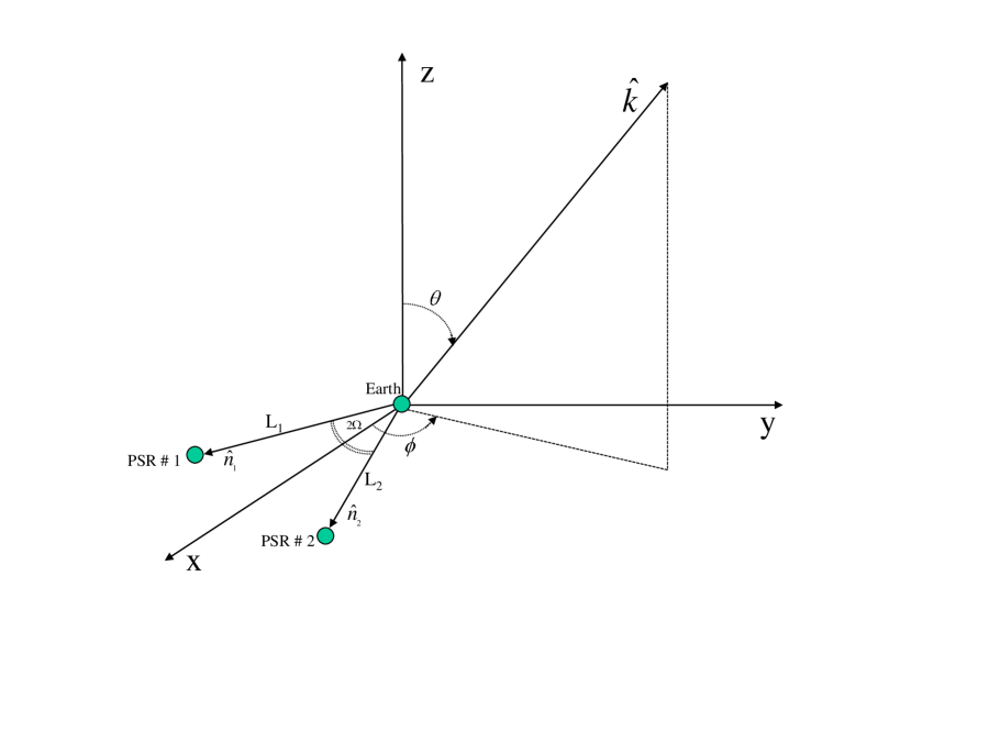
Figure 1: Two millisecond pulsars are tracked simultaneously by two radio telescopes sited near each other. The unit vector ${\bf{\hat{k}}}$ defines the direction of propagation of the gravitational wave signal and ($\theta,\phi$) are the usual polar angles associated with it. The two unit vectors, (${\bf{\hat{n}}}_{1},{\bf{\hat{n}}}_{2}$), define the directions in the sky to the two pulsars, and the angle between them has been denoted with $2\Omega$. The bisector of this angle coincides with the $x$-axis of an orthogonal coordinate system in which the $y$-axis lies in the plane defined by the two unit-vectors (${\bf{\hat{n}}}_{1},{\bf{\hat{n}}}_{2}$), and the $z$-axis is chosen to form a right-handed orthogonal triplet ($x,y,z$).

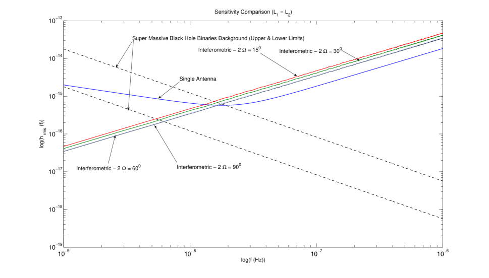
Figure 2: Sensitivity of the interferometric pulsar timing technique as a function of the Fourier frequency and for various values of the pulsars angular separation in the sky, $2\Omega$. The pulsars have been assumed to be at equal distance from Earth ($1$ kpc). Note the mild dependence of the sensitivity over the angle $2\Omega$ in the interval of values considered. The sensitivity of a single-telescope experiment (blue curve), as well as the current estimates of the upper and lower bounds on the characteristic amplitude radiated by an ensemble of super-massive black-hole binaries (two black dashed-lines) are included. See text for details.

In Figure (2) we plot the sensitivity of the interferometric pulsar timing technique as a function of the Fourier frequency and for various values of the angle $2\Omega$ enclosed between the directions to the two pulsars. For sake of simplicity we have assumed the two pulsars to be at an equal distance of $1$ kpc from Earth. We have independently analyzed configurations with unequal distances and found no significant differences to the sensitivity curves shown in Fig.(2). Another property of the sensitivity curves is their mild dependence over the angle $2\Omega$; a configuration with two millisecond pulsars that are separated by only $15^{0}$ in the sky shows a sensitivity that is only $28$ percent worst than that with $2\Omega=90^{0}$. However, for values of $2\Omega$ smaller than $15^{0}$, the sensitivity rapidly worsen and goes to zero at $2\Omega=0$. This is of course consequence of having assumed, for this calculation, the two pulsars to be at equal distance from Earth. In the case when $L_{1}\neq L_{2}$ instead, the sensitivity to gravitational radiation does not go to zero at $2\Omega=0$, as it can be easily understood by simple inspection of Eq. (3). Since longer joint tracking times can be achieved with pairs of millisecond pulsars that have smaller angular separation, our analysis indicates that these configurations (with, let’s say $2\Omega\simeq 20^{0}$) might be preferable to those with larger angle $2\Omega$.

For comparison, in Fig.(2) we have included the sensitivity of a single-telescope experiment that relies on a LITS clock JAT2011 . Although at frequencies larger than about $10^{-8}$ Hz this is about a factor of $2$ better than that of the interferometric technique (in this part of the band the noises affecting the interferometric combination are twice as many), at frequencies lower than $10^{-8}$ Hz the advantage of the interferometric technique becomes evident. In this region of the band the clock noise dominates all other noise sources in a single-telescope timing residuals data, and our technique exactly cancels it.

In order to put in perspective the sensitivity enhancement brought by the interferometric pulsar timing technique over single-telescope experiments, we have included the current estimated range of strengths of an astrophysical gravitational wave background from incoherently radiating super-massive black hole binaries Black1 ; Black2 . At $3\times 10^{-9}$ Hz we find that the most conservative prediction of the strength of such a background would result into an ${\rm SNR}\simeq 5$, while a more optimistic estimate of its characteristic strain amplitude would make it detectable with a ${\rm SNR}\simeq 50$.

References

- (1) K.S. Thorne. In: Three Hundred Years of Gravitation, 330-458, Eds. S.W. Hawking, and W. Israel (Cambridge University Press: New York), (1987).
- (2) http://www.ligo.caltech.edu/ .
- (3) http://www.virgo.infn.it/ .
- (4) http://www.geo600.uni-hannover.de/ .
- (5) http://tamago.mtk.nao.ac.jp/ .
- (6) J.W. Armstrong, Living Rev. Relativity, 9, (2006). URL (cited on May 20, 2010): http://www.livingreviews.org/lrr-2006-1 .
- (7) P. Bender, K. Danzmann, & the LISA Study Team, Laser Interferometer Space Antenna for the Detection of Gravitational Waves, Pre-Phase A Report, MPQ233 (Max-Planck- Institüt für Quantenoptik, Garching), July 1998.
- (8) S. Detweiler, Ap. J., 234, 1100-1104 (1979).
- (9) F.A. Jenet, J.W. Armstrong and M. Tinto, Phys. Rev. D, Rapid Communications: submitted for publication. Also available at: http://arxiv.org/abs/1101.3759
- (10) J. Stuart B. Wyithe, and A. Loeb, Ap. J., 590, 691-703 (2003)
- (11) M. Enoki, K.T. Inoue, M. Nagashima, and N. Sugiuama, Ap. J., 615, 19-28 (2004).
- (12) R.W. Hellings, and G.S. Downs, Ap. J., 265, L39-L42 (1983).
- (13) F.A. Jenet, G.B. Hobbs, K.J. Lee, and R.N. Manchester Ap. J., 625, L123-L126 (2005).
- (14) F.B. Estabrook and H.D. Wahlquist, Gen. Relativ. Gravit., 6,439 (1975).
- (15) W.L. Burke, Ap. J., 196, 329 (1975).
- (16) H.D. Wahlquist, Gen. Relativ. Gravit., 19, 1101 (1987).
- (17) J.P.W. Verbiest, M. Bailes, W.A. Coles, G.B. Hobbs, W. van Straten, D.J. Champion, F.A. Jenet, R.N. Manchester, N.D.R. Bhat, J.W. Sarkissian, D. Yardley, S. Burke-Spolaor, A.W. Hotan, and X.P. You, Mon. Not. R. Astron. Soc., 400, 951-968 (2009).
- (18) J.W. Armstrong, F.B. Estabrook and M. Tinto, Ap. J., 527, 814 (1999).