$F_{K}/F_{\pi}$ from the Budapest-Marseille-Wuppertal Collaboration

A. Ramos^a, S. Dürr^b,c, Z. Fodor^b,c,d, C. Hoelbling^b, S. D. Katz^b,d, S. Krieg^b, T. Kurth^b, L. Lellouch^a, T. Lippert^b,c, K. K. Szabó^b
[Budapest-Marseille-Wuppertal Collaboration]

^aCentre de Physique Théorique. CNRS Luminy, Case 907, F-13288 Marseille Cedex 9, France.

^bBergische Universität Wuppertal, Gaussstr. 20, D-42119 Wuppertal, Germany.

^cJülich Supercomputing Center, Forschungszentrum Jülich, D-52425 Jülich, Germany.

^dInstitute for Theoretical Physics, Eötvös University, H-1117 Budapest, Hungary.

Based on a series of lattice calculations we determine the ratio $F_{K}/F_{\pi}$ in QCD. With experimental data from kaon decay and nuclear double beta decay, we obtain a precise determination of $|V_{us}|$. Our simulation includes $2+1$ flavours of sea quarks, with three lattice spacings, large volumes and a simulated pion mass reaching down to about 190 MeV for a full control over the systematic uncertainties.

PRESENTED AT

Proceedings of CKM2010, the 6th International Workshop on the CKM Unitarity Triangle, University of Warwick, UK, 6-10 September 2010.

1 Introduction

The measurement of CKM matrix elements involves examining weak decays of hadrons. The theoretical description of these decays involves computing strongly interacting effects of quarks and gluons inside the hadrons. These effects should be determined in a fully non-perturbative way. Any weak decay can be written as the product of three factors

$$\textrm{Weak decay}=\{\textrm{Kinematic}\}\times\{\textrm{CKM element}\}\times\{\textrm{Non-perturbative QCD}\}.$$ (1)

Computing the non-perturbative QCD effects is a difficult task. A first principle analytical approach does not yet exists. We have to live either with numerical simulations or with models of QCD.

Here we will use lattice QCD as a numerical tool to compute non perturbative QCD meson decay contants.

1.1 Light meson decay constants and $|V_{us}|$

We will follow a proposal by Marciano [1] of examining the ratio of decay widths

$${\Gamma(K\to\mu\overline{\nu}_{\mu})\over\Gamma(\pi\to\mu\overline{\nu}_{\mu})}={|V_{us}|^{2}\over|V_{ud}|^{2}}\frac{F_{K}^{2}}{F_{\pi}^{2}}{M_{K}(1-m_{\mu}^{2}/M_{K}^{2})^{2}\over M_{\pi}(1-m_{\mu}^{2}/M_{\pi}^{2})^{2}}\left\{1+{\alpha\over\pi}(C_{K}-C_{\pi})\right\}$$ (2)

where this ratio, even including electromagnetic corrections, are experimentally know with an $0.4\%$ precision. Masses are known at least with a relative precision of $3\!\times\!10^{-5}$. This implies that an accurate determination of the ratio $F_{K}/F_{\pi}$ can be used to determine $|V_{us}|/|V_{ud}|$. The most recent update of the Flavianet kaon working group is [2]:

$${|V_{us}|\over|V_{ud}|}\,{F_{K}\over F_{\pi}}=0.27599(59)\;.$$ (3)

This may be used with $|V_{ud}|=0.97425(22)$ [3] from super-allowed nuclear $\beta$ decays and the lattice determination of $F_{K}/F_{\pi}$ to obtain $|V_{us}|$.

2 Simulation details

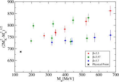
We simulate 2 degenerate light clover fermions representing the $u$ and $d$ quarks in the strong isospin limit plus a third heavier clover fermion that represents the strange quark. Whereas the value of the strange quark mass is held fixed close to its physical value light quark masses are varied through a significant range so that our $\pi$ mesons have masses in the range $190\textrm{ MeV}\raise 1.29167pt\hbox{$<$\kern-7.5pt\raise-4.73611pt\hbox{$\sim$}}M_{\pi}\raise 1.29167pt\hbox{$<$\kern-7.5pt\raise-4.73611pt\hbox{$\sim$}}460\textrm{ MeV}$. This allows a controlled extrapolation to the physical point $M_{\pi}\approx 135\textrm{ MeV}$ (see Figure 1a).

(a) Overview of our simulation points in the plane $(M_{\pi},\sqrt{2M_{K}^{2}-M_{\pi}^{2}})$.

(b) One of the 1512 fits that leads to our final determination of $F_{K}/F_{\pi}$

Figure 1: Overview of simulation points and a representative fit.

We simulate at three different lattice spacings $a\!\simeq\!0.124\textrm{ fm}$ $(\beta=3.3)$, $a\!\simeq\!0.083\textrm{ fm}$ $(\beta=3.57)$, and $a\!\simeq\!0.065\textrm{ fm}$ $(\beta=3.7)$ for a controlled extrapolation to the continuum limit.

All our simulations are done in large volumes $M_{\pi}L\raise 1.29167pt\hbox{$>$\kern-7.5pt\raise-4.73611pt\hbox{$\sim$}}4$, so that finite volume corrections are below $1\%$.

More details about both our fermion and gauge actions can be found in [4].

3 Systematic uncertainties.

To obtain a QCD results from lattice data one has to perform several extrapolations: one has to extrapolate data to the physical value of the quark masses (chiral extrapolation), one has to to the infinite volume limit, and to the continuum limit. One has also to deal with the contribution from exited states and the possible uncertainty associated with determining the QCD coupling (i.e. setting the scale). All these considerations should be taken into account and each of them should be reflected in the final uncertainty of our result.

A detailed description of the method sketched here can be found in the original work [5].

3.1 Scale setting issues

$2+1$ flavour QCD has three independent parameters: the light quark masses, the strange quark mass, and the gauge coupling. One needs three experimental inputs to fix these parameters in our simulations.

To fix quark masses one uses the experimental values of the masses of the $\pi$ and K mesons, $M_{\pi}$ and $M_{K}$.

To set the lattice spacing, one uses a physical state whose mass does not strongly depend on quark masses. We used both the $\Omega$ and $\Xi$ states, the differences between these two choices measures the error associated with our choice of physical input.

All physical inputs are corrected to take into account that we simulate in the isospin symmetric limit without electromagnetic interactions.

3.2 Chiral extrapolation

There exist basically two approaches that can guide us in the extrapolation to the physical point. We can use an effective field theory approach ($\chi$PT), either in the two or three flavour setups.

Another possibility comes from the observation that physical quantities like decay constants or masses have an analytical expansion in the quark masses as long as this expansion performed around a regular point far from the singular point $m_{q}=0$. If our lattice data is close enough to the physical point these analytical expansions should be a fair approximation to the behaviour of the physical quantity up to the physical point.

We will fit our data to a total of 7 different expressions that correspond to one of the previously mentioned approaches.

For the case of three flavour $\chi$PT our data is well fitted using the NLO relation for the ratio $F_{K}/F_{\pi}$ [6]. In fact up to higher order terms, the NLO relation can be written in three different ways. The difference between these three expressions measures the contribution of higher order contributions.

The ratio $F_{K}/F_{\pi}$ can be obtained from the pion mass dependence of $F_{K}$ in the heavy kaon two flavour $\chi$PT formalism and the pion mass dependence of $F_{\pi}$ in $SU(2)$ $\chi$PT [7]. Our data is well fitted by the NLO relation, and up to higher order terms, we have two different ways of expanding the ratio of decay constants. The difference between these two expressions are higher order contributions.

Finally the ratio of decay constants have a perfectly regular expansion, as soon as this expansion is done far from the singular point $m_{q}=0$. In fact our lattice data is well fitted by a simple polynomial expansion around a regular point that lies midway between the physical point and our heaviest pion ensemble. One can also fit the data to a rational approximation, that can be seen as a Padé like ansatz. This gives a total of 2 expressions based on an analytical expansion around a regular point that, again, differ in higher order terms.

It is important to remark that the total of 7 formulae differ both in the approach (three, two flavour $\chi$PT or analytical expansions), and in the higher order contributions within a framework (NNLO contributions in $\chi$PT or higher powers in the analytical expansions.)

3.3 Continuum limit

The ratio $F_{K}/F_{\pi}$ is a flavour breaking term. This means that no matter the value of the lattice spacing we will always have $F_{K}/F_{\pi}=1$ when $m_{ud}=m_{s}$. This suggests that cutoff effects should be $\propto(M_{\pi}^{2}-M_{K}^{2})$.

Our action is formally only improved up to order $\mathcal{O}(\alpha_{s}a)$, but we have numerical evidence [4] that cutoff effects scale as $\mathcal{O}(a^{2})$.

In particular for the present case, cutoff effects are small. This can be understood by looking at $SU(3)$ $\chi$PT, where the leading correction cancels for the ratio of decay constants. For our particular dataset they are statistically consistent with zero (i.e. the statistical uncertainty of our data are bigger than lattice spacing corrections.)

Taking these considerations into account we choose to parametrise cutoff effects in our data by adding or not a term

$$\left.\frac{F_{K}}{F_{\pi}}\right|_{\textrm{c.o.}}=c\times\left\{\begin{array}[]{l}a(M_{K}^{2}-M_{\pi}^{2})/\mu_{\textrm{QCD}}\\ \quad\textrm{or}\\ a^{2}(M_{K}^{2}-M_{\pi}^{2})\\ \end{array}\right.$$ (4)

to any of the previous 7 formulae that gives the dependence of $F_{K}/F_{\pi}$ with meson masses.

3.4 Finite volume corrections

For large enough lattices, finite volumes effects scale as $\propto e^{-M_{\pi}L}$. All our simulation points respect the bound $M_{\pi}\raise 1.29167pt\hbox{$>$\kern-7.5pt\raise-4.73611pt\hbox{$\sim$}}4$, making finite volume corrections small. In fact our data is well fitted without any kind of finite volume correction, indicating that the size of the correction is smaller than the statistical accuracy of our data.

Nevertheless, corrections due to finite volume are known in $\chi$PT. Meson masses and decay constants receive corrections that have been computed. We decided to correct the decay constants with a 2 loop expression [8]. To estimate the uncertainty of this correction, we use the 1 loop expression together with an upper bound on the correction (coming from correcting only $F_{\pi}$).

3.5 Excited state contributions

Masses and decay constants are obtained from the large time behaviour of correlators, i.e.

$$C(t)\equiv\left(\frac{a}{L}\right)^{3}\sum_{\vec{x}}\langle[\overline{d}\gamma_{5}u](x)[\overline{u}\gamma_{5}d](0)\rangle\stackrel{{\scriptstyle 0\ll t\ll T}}{{\longrightarrow}}\frac{\langle 0|\overline{d}\gamma_{5}u|\pi^{+}(\vec{0})\rangle\langle\pi^{+}(\vec{0})|\overline{u}\gamma_{5}d|0\rangle}{2M_{\pi}}\,e^{-{M_{\pi}}t}.$$ (5)

We choose for each value of the coupling $\beta$ the start of the fitting interval $t_{\textrm{min}}$ so that it is strongly dominated by the ground state. There are several reasonable possibilities for this, and we choose to use 18 possibilities that will receive different tiny contributions from excited states. These different fitting intervals will be used to estimate the uncertainties due to excited state.

4 Results

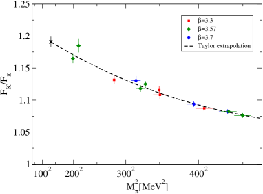
The procedure described above lads to a total of $2\times 18\times 7\times 2\times 3=1512$ different ways of obtaining the ratio $F_{K}/F_{\pi}$ in the continuum, at the physical mass point and in the infinite volume limit (see Figure 1b.)

Since not all the previous procedures describes our data equally well (although the $\chi^{2}/\textrm{dof}$ for all the fits is close to 1), we weight each of the values with the quality of the fit to produce a distribution of values.

The median, typical result of our analysis, is taken as our final result. The 16-th/84-th percentiles, that measures the “spread” of values, give our final systematic uncertainty. To determine the statistical accuracy of our results, we resample our configurations 2000 times, and the standard deviation of the median over these 2000 samples is taken as the statistical uncertainty.

Our final result is

$${F_{K}\over F_{\pi}}\bigg{|}_{\textrm{phys}}=1.192(7)_{\textrm{stat}}(6)_{\textrm{syst}}$$ (6)

Using the value $|V_{ud}|=0.97425(22)$[3] we obtain

$$|V_{us}|=0.2256(18).$$ (7)

Using also $|V_{ub}|=(3.93\pm 0.36)\times 10^{-3}$ the first row CKM unitarity relation is

$$|V_{ud}|^{2}+|V_{us}|^{2}+|V_{ub}|^{2}=1.0001(9)$$ (8)

with no signal for physics beyond the standard model. For details on the calculations see [5].

References

- [1] William J. Marciano. Phys. Rev. Lett., 93:231803, 2004.
- [2] M. Antonelli et al. Nucl. Phys. B Proc. Suppl., 81:181–183, 2008.
- [3] J. C. Hardy and I. S. Towner. Phys. Rev., C79:055502, 2009.
- [4] S. Durr et al. Phys. Rev., D79:014501, 2009.
- [5] S. Durr et al. Phys. Rev., D81:054507, 2010.
- [6] J. Gasser and H. Leutwyler. Nucl. Phys., B250:517–538, 1985.
- [7] C. Allton et al. Phys. Rev., D78:114509, 2008.
- [8] Gilberto Colangelo, Stephan Durr, and Christoph Haefeli. Nucl.Phys., B721:136–174, 2005.