∎
Universitat Politècnica de Catalunya,
c/Esteve Terrades 5, 08860 Castelldefels, Spain
Institut d’Estudis Espacials de Catalunya,
c/Gran Capità 2–4, Edif. Nexus 104, 08034 Barcelona, Spain
22email: marc.diaz.aguilo@fa.upc.edu, garcia@fa.upc.edu 33institutetext: Alberto Lobo 44institutetext: Institut de Ciències de l’Espai, CSIC,
Campus UAB, Facultat de Ciències,
Torre C-5, 08193 Bellaterra, Spain
Institut d’Estudis Espacials de Catalunya,
c/Gran Capità 2-4, Edif. Nexus 104, 08034 Barcelona, Spain
44email: lobo@ice.cat
Neural network interpolation of the magnetic field for the LISA Pathfinder Diagnostics Subsystem
Abstract
LISA Pathfinder is a science and technology demonstrator of the European Space Agency within the framework of its LISA mission, which aims to be the first space-borne gravitational wave observatory. The payload of LISA Pathfinder is the so-called LISA Technology Package, which is designed to measure relative accelerations between two test masses in nominal free fall. Its disturbances are monitored and dealt by the diagnostics subsystem. This subsystem consists of several modules, and one of these is the magnetic diagnostics system, which includes a set of four tri-axial fluxgate magnetometers, intended to measure with high precision the magnetic field at the positions of the test masses. However, since the magnetometers are located far from the positions of the test masses, the magnetic field at their positions must be interpolated. It has been recently shown that because there are not enough magnetic channels, classical interpolation methods fail to derive reliable measurements at the positions of the test masses, while neural network interpolation can provide the required measurements at the desired accuracy. In this paper we expand these studies and we assess the reliability and robustness of the neural network interpolation scheme for variations of the locations and possible offsets of the magnetometers, as well as for changes in environmental conditions. We find that neural networks are robust enough to derive accurate measurements of the magnetic field at the positions of the test masses in most circumstances.
Keywords:
LISA Pathfinder magnetometers on-board instrumentation spaceborne and space-research instruments neural networks1 Introduction
LISA (Laser Interferometer Space Antenna) is a joint ESA/NASA space mission aimed at detecting low frequency gravitational waves, in the range between 10-4 Hz and 1 Hz. LISA will be a constellation of three spacecraft which occupy the vertexes of an equilateral triangle, with sides of 5 million kilometers. The barycenter of the constellation will revolve around the Sun in a quasi circular orbit, inclined 1∘ with respect to the ecliptic, and trailing the Earth by some 20∘, about 45 million kilometres. Each spacecraft harbors two proof masses, carefully protected against external disturbances such as solar radiation pressure and charged particles, which ensures they are in nominal free-fall in the interplanetary gravitational field. Gravitational waves show up as differential accelerations between pairs of proof masses in distant spacecrafts, and the working principle of LISA is to measure such accelerations using picometer precision laser interferometry. The interested reader is referred to references bib:axel and bib:bill for more extensive information, as well as to the LISA International Science Team (LIST) webpage bib:web .
The technologies required for the LISA mission are many and very challenging. This, coupled with the fact that some flight hardware cannot be tested on ground since free fall conditions cannot be maintained during periods of hours, led to set up a technology demonstrator to test critical LISA technologies in a flight environment. These technologies will be tested in a precursor mission, which is called LISA Pathfinder (LPF). This mission is framed within the Scientific Program of ESA, and it is expected to be launched towards early 2012. The idea of LPF is to squeeze one LISA arm from five million kilometers to 35 centimeters, then determine the noise of the measurements in a frequency range which is slightly less demanding than that of LISA. More specifically, the requirement is formulated in terms of spectral density of acceleration noise as
| (1) |
for 1 mHz 30 mHz, where is the frequency in Hz.
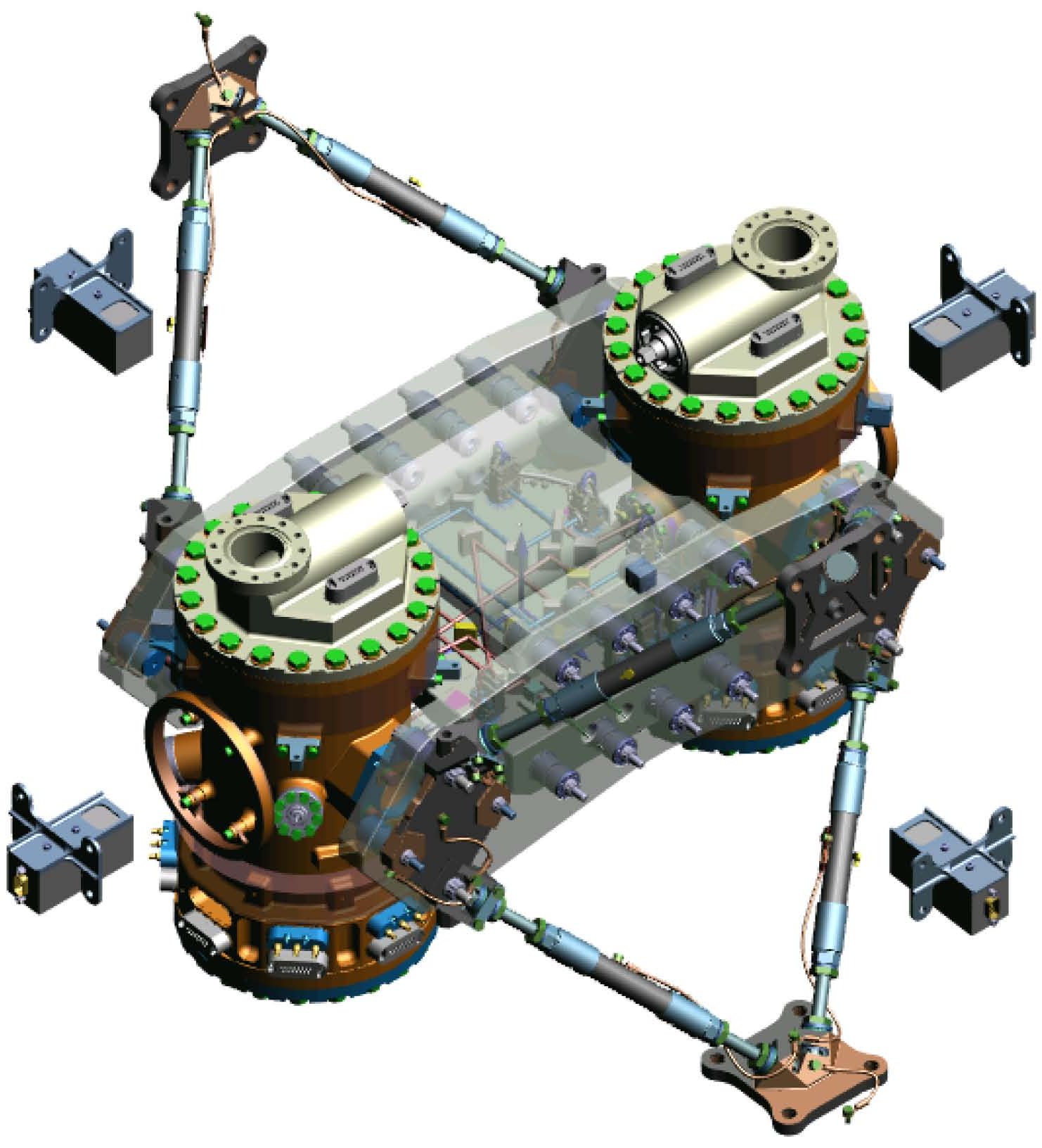
The payload on board LPF is called the LISA Technology Package (LTP) bib:anza . Its main components are the two gravitational reference sensors, which are the two large vertical cylinders in figure 1. In this figure it can also be seen the optical metrology subsystem, which provides picometer precision measurements of the relative position and acceleration of the two test masses, using precise interferometry. This system is located between the two gravitational reference sensors. Also visible, and specially relevant here, are the four tri-axial magnetometers, which are represented as floating boxes. Their actual physical support is the lateral wall of a (not drawn) larger cylinder which encloses the entire LTP.
Magnetic noise in the LTP is required to be not more than 40% of the total readout noise, i.e., m s-2 Hz-1/2 out of m s-2 Hz-1/2 in the measurement bandwidth, see Eq. (1). This noise appears because the residual magnetization and susceptibility of the test masses couple with the surrounding magnetic field, giving rise to a force in each of them
| (2) |
In this expression B is the magnetic field in the test mass, M is its density of magnetic moment (magnetization), is the volume of the test mass, is its magnetic susceptibility, is the vacuum magnetic constant ( m kg s-2 A-2), and indicates the volume average of the enclosed quantity. As clearly seen from Eq. (2), there are two sources of magnetic noise. The first one is due to the fluctuations of the magnetic field and its gradient in the regions occupied by the test masses bib:LISA . The second one comes from the susceptibility of the test mass and the magnetic remanence fluctuations bib:ntcs . This additional noise is expected to be much less important, and it is usually disregarded.
Clearly, a quantitative assessment of magnetic noise in the LTP requires real-time monitoring of the magnetic field and its gradient bib:trento . This is the ultimate goal of the tri-axial fluxgate magnetometers bib:DDS_LTP . These devices have a high permeability magnetic core, which drives a design constraint to keep them somewhat far from the test masses. Thus, their readouts do not provide a direct measurement of the magnetic field at the position of the test masses, complicating the task of inferring the field at their position, and forcing the implementation of an interpolation method to overcome this shortcoming. However, such interpolation process faces serious difficulties. Indeed, the size of the interpolation region, that is, the interior of the LTP Core Assembly (LCA), is too large for a linear interpolation scheme to be reliable. Additionally, the number of magnetometer channels does not provide sufficient data to go beyond a poor linear approximation bib:myPaper . However, the structure of the magnetic field is rather complex, as the sources of magnetic field are essentially the electronic components inside the spacecraft. The number of identified sources is about 50, and they behave as magnetic dipoles, the only exception being the solar panel, which is best approximated by a quadrupole. The positions of the sources are dictated by the architecture of the satellite, which defines the exact position of each electronic subsystem. Fortunately, there are no sources of magnetic field inside the LCA, all being placed within the spacecraft, but outside the LCA walls. Adequate processing of all the available information shows that the magnetic field is smaller towards the center of the spacecraft (where the test masses are located) than it is in its periphery (where the magnetometers take measurements).
It has been recently shown bib:myPaper that since the standard interpolation scheme, which is based in multipole expansion of the magnetic field inside the LCA volume, does not go beyond quadrupole order, its performance in estimating the magnetic field and its gradients is very poor. On the contrary, artificial neural networks have been shown to be a reliable alternative to estimate the required field and gradient values at the positions of the test masses. The reasons for this are multiple. Firstly, the multipole expansion only takes into account the readings of the magnetometers, whereas the artificial neural network also uses the actual value of the magnetic field at the position of the test masses to train the network. This is a crucial issue since the interpolation algorithm is fed with additional information. Secondly, the classical interpolation method seeks for a global solution of the magnetic field. That is, the multipole expansion models the magnetic field inside the entire volume of the LCA. Clearly, since the available information for the multipole expansion is rather limited, the quality of the global solution is very poor. In sharp contrast, the artificial neural network first finds and then uses the correlation between the magnetic field at the positions of the magnetometers and the test masses to obtain reliable values of the magnetic field for any magnetic configuration. As a matter of fact, the artificial neural network performs a point-to-point interpolation and it is not aimed at reproducing the highly non-linear magnetic field well at any arbitrary position within the volume of the LCA. Finally, artificial neural networks are trained using a large number of magnetic field realizations, thus the interpolating algorithm uses a statiscally elaborated information. In this sense, it is important to realize that artificial neural networks have been shown to be a robust and easily implementable technique among numerous statistical modeling tools bib:kecman . On the contrary, the multipole expansion does not use statistical information. Once the readings of the magnetometers are known, the theoretical solution for the magnetic field within the entire volume of the LCA is determined in a straightforward way.
Nevertheless, an in depth study of how the results of the interpolation procedure depend on the specific characteristics of the neural network remains to be done. It also remains to further investigate why the neural network — which uses lineal transfer functions — obtains such good results interpolating the value of the magnetic field at the positions of the test masses, which are well inside a deep well of magnetic field. Finally, an assessment of the robustness of the neural network interpolating scheme in front of the unavoidable errors in the positions of the magnetometers, or in front of low-frequency variations of the magnetic environment and, more importantly, in front of offsets in the readings of the magnetometers still is needed. These are precisely the goals of this paper.
The paper is organized as follows. In Sect. 2 we discuss the appropriateness of our neural network approach to measure the magnetic field and its gradients at the positions of the test masses, and we discuss which are the accuracies obtained when different architectures of the neural network are adopted. It follows Sect. 3, where we discuss how the unavoidable errors in the onground measurements of the magnetic dipoles of each electronic box affect the performance of the adopted neural network. In Sect. 4 we evaluate the expected errors in the estimate of the magnetic field and its gradients due to a possible offset in the readings of the magnetometers due to launch stresses, whereas in Sect. 5 we study how the mechanical precision of the positions of the tri-axial magnetometers and their spatial resolution affect the determination of the magnetic field and its gradients. Sect. 6 is devoted to assess the reliability of our neural network approach in front of a slowly varying magnetic environment. Finally, in Sect. 7 we summarize our main findings, we discuss the significance of our results and we draw our conclusions.
2 The neural network architecture
Although neural networks have been used in different space applications bib:scatterometer ; bib:satellite , to the best of our knowledge this is the first application of neural networks to analyze inflight outputs in space missions. Hence, studying the robustness of the neural network architecture proposed to estimate the magnetic field inside the LCA is a mandatory task.
2.1 The fiducial neural network architecture

Fig. 2 shows a simplified version of the fiducial architecture of our neural network. As can be seen, the number of inputs is twelve — one for each magnetometer readout — corresponding to the four tri-axial magnetometers placed in the spacecraft. These readings are the only valuable information which can be used to estimate the magnetic field at the positions of the test masses, and constitute the input layer of the neural network. On the other hand, to estimate the magnetic field three outputs will be required — corresponding to the three field components per test mass — whereas to estimate the gradient only five additional outputs are needed. This is because the magnetic field has zero divergence and zero rotational. Thus, the gradient matrix is a traceless symmetric matrix, and therefore only 5 out of its 9 components are independent. These outputs are the output layer of the neural network. In addition to the two previously described layers, there is only one intermediate layer, which constitutes the hidden layer. This layer is made of 15 neurons. Using this architecture for the neural network the magnetic field estimates typically have standard deviations on the order of bib:myPaper , a value to which we compare the results of our analysis.
2.2 Training and testing
Training and testing data sets were simulated using the most complete and up-to-date information about the magnetic configuration within the spacecraft. The complete magnetic configuration of the satellite has not been measured yet, because some units have not been delivered yet to the prime contractor. Nevertheless, the exact position of each unit in the spacecraft reference frame is known. On the other hand, the magnetic moments used in our simulations are those reported by the constructors of each subsystem. Unfortunately, this data is not available yet for all units, and moreover although the moduli of the dipoles are known for all the subsystems their directions are not known yet for most of the units. The three-dimensional values of the magnetic dipoles of each unit will be accurately measured in the final testing campaign to be performed on each subsystem before assembling. This campaign is expected to be performed on the assembled spacecraft during 2011. The training and validation of the neural network using the measured values of the magnetic dipoles will be done after the campaign but the specific details of the processing algorithm are expected to remain unchanged. Moreover, the magnetic field inside the LCA is expected to vary substantially between the different operational modes. Accordingly, since the magnetic configuration of the spacecraft may have different characteristics for different operational modes, it is foreseen that a different neural network will be trained for each of these configurations.
Given the unknown orientations of the magnetic dipoles we generate several magnetic configurations assigning randomly the orientations of the 46 dipoles. An example scenario is thus characterized by a selection of the 46 dipoles with random orientations. The random character of the procedure may seem unrealistic, since the actual satellite configuration is not random. In this context, however, randomness is an efficient way of mimicking our lack of knowledge of all the directions of the sources of magnetic field. Nevertheless, it is worth mentioning that the produced sets are consistent with our expectations and the mission requirements bib:LISA ; bib:DDS_LTP since at the positions of the test masses we obtain magnetic fields nT, while the readings at the magnetometers are of the order of 4 to 10 T. With this approach the magnetic field generated by the dipole distribution at a generic point x and time is therefore given by
| (3) |
where na = / are unit vectors connecting the the -th dipole ma with the field point x, and is the number of dipoles. In order to simulate realistic magnetic environments, we compute the magnetic field at the positions of the magnetometers and at the positions of the test masses using Eq. (3). The positions of the test masses and of the magnetometers are shown in table 1. Two different batches of samples are generated. The first batch was used as the training set for a neural network with the architecture of Fig. 2. This batch consists in 12 inputs (3 inputs for each of the 4 vector magnetometers) and 16 outputs representing the field information at the position of the two test masses (3 field plus 5 gradient components per test mass). The second batch has been used for validation to assess the performance of the neural network.
| Test masses | [m] | [m] | [m] |
|---|---|---|---|
| 1 | 0.1880 | 0 | 0.4784 |
| 2 | 0.1880 | 0 | 0.4784 |
| Magnetometers | [m] | [m] | [m] |
| 1 | 0.0758 | 0.3694 | 0.4784 |
| 2 | 0.3765 | 0 | 0.4784 |
| 3 | 0.0758 | 0.3694 | 0.4784 |
| 4 | 0.3765 | 0 | 0.4784 |
2.3 Varying the number of neurons

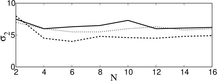
Assesing the correct choice of the number of neurons of a neural network is not a simple task. When the neural network is composed by only one hidden layer, the input layer contains as many inputs-neurons as the information we provide to the network and as many output-neurons as the target information we want to reconstruct. Nevertheless, as far as the number of neurons of the hidden layer is concerned, it is not guaranteed that the architecture of the selected neural network is optimal nor there is an algorithm in the current literature to determine the optimal number of neurons bib:neuralPrunning ; bib:size . Normally, to obtain good results, the smallest system obtained after prunning that is capable to fit the data should be used. Unfortunately, it is not obvious what size is best. A system with a small number of neurons will not be able to learn from the data, while one with a large number of neurons may learn very slowly and, moreover, it will be very sensitive to the initial conditions and learning paramaters. Additionally, it should be taken into account that one of the biggest problems of large networks for some specific problems is the fact that in the early stages of training, the error on both the training and tests tends to decrease with time as the network generalizes for the examples to the underlying function. However, at some point, the error on the testing set reaches a minimum and begins to increase again as the network starts to adapt to artifacts and specific details in the training data, while the training error asymptotically decreases. This problem, known as overfitting, occurs more frequently in large networks due to the excessive number of degrees of freedom in comparison to the training set bib:overfitting . To avoid this, we have used the early stopping technique, which overcomes this shortcoming.
In the early stopping technique the available data is divided into three subsets bib:kecman . The first subset is the training set, which is used for computing the gradient and updating the network weights and biases. The second subset is the validation set. The error on the validation set is monitored during the training process. The validation error normally decreases during the initial phase of training, as does the training set error. However, when the network begins to overfit the data, the error on the validation set typically begins to rise. When the validation error increases for a specified number of iterations, the training is stopped, and the weights and biases at the minimum of the validation error are returned to the values obtained at the minimum. All these precautionary measures avoid overfitting. Therefore, the analysis of the number of neurons needed for the hidden layer can be made analyzing the evolution of the estimation error on the testing set as the number of neurons increases. The results of such an analysis are depicted in figure 3, which shows the standard deviation of the estimate for both test mass 1, , and test masss 2, as a function of the number of neurons in the hidden layer, .
| TM1 | TM2 | |||||
|---|---|---|---|---|---|---|
| Function | ||||||
| Tangent sigmoid | 4.1 | 3.8 | 2.5 | 5.9 | 5.2 | 4.5 |
| Linear | 3.8 | 3.5 | 2.3 | 5.7 | 5.4 | 4.2 |
| Logarithmic sigmoid | 4.2 | 3.8 | 2.5 | 6.2 | 5.1 | 4.5 |
| Radial base | 4.2 | 4.3 | 3.9 | 6.3 | 6.0 | 4.8 |
| Step | 7.5 | 7.6 | 4.9 | 12.3 | 8.2 | 7.9 |
As can be seen in this figure, when a reduced number of neurons is used the model cannot accurately estimate the underlying function due to the lack of tunnable parameters. As the number of neurons in the hidden layer is increased, the neural network performs better and for a number of neurons larger than 15 the error is not further reduced. Consequently, we conclude that for this specific application the adequate number of neurons for the hidden layer lies between 10 and 15. This choice ensures a network large enough to be capable of estimating the underlying relationship and not excessively large to consume excessive training time, learn slowly and be dependent on the learning algorithm. We have also checked that increasing the number of hidden layers of the neural network does not result in a better performance of the interpolating algorithm, but for the sake of conciseness we do not show the results here. All in all, it seems that our fiducial architecture seems to work best.
2.4 Changing the type of neuron
Most of the feed-forward networks are trained with the back-propagation algorithm and gradient descent techniques are used to minimize some specific cost function, and this has been the case for the training algorithm used here. This means that all activation functions within the network must be differentiable to be able to compute the network gradient for each learning step. Normally, the most commonly used type of functions are the tangent sigmoid or the logarithmic sigmoid bib:kecman , which can model any non-linear function if properly trained bib:dreyfus , whereas linear functions are usually employed for linear models with high dimensionality.
We have studied several possibilities and the results are listed in table 2, where we show for the different types of neurons the standard deviations of the probability density functions of the estimates of the magnetic field for both test mass 1 and 2 (TM1 and TM2, respectively). In our case, and as borne out from table 2, the linear function together with the tangent sigmoid and the logarithmic sigmoid are the most efficient choices, while the performance of the radial base function is slightly worse. Finally, the step function (the popular perceptron) does not yield good results because it is specifically designed to be used for classification problems. Specifically, the linear neuron is the one for which we obtain the best results. This could be surprising given that our problem is highly non-linear. The reason is that for every magnetic configuration there exists a large and fairly stable difference between the value of the magnetic field at the location of the magnetometers (all of the components of the magnetic field are T) and the field at the position of the test masses (all the components are on the 100 nT level). For this reason, the weigths of the network happen to be the most relevant modeling factors. That is, the point-to-point interpolation can be understood in the linear case as a simple weighted sum of the magnetometers measurements. Accordingly, because of its simplicity and good results, we use the linear function as the basic unit in our regression study. It is worth noting at this point that similar results could be obtained using a high-dimensionality least squares analysis, but in our specific case we have found matrix inversion problems because some magnetometer channels present highly correlated signals.
2.5 Underlying structures
We have already shown that our neural network is highly reliable. Thus, it is normal to ask ourselves which is the ultimate reason of this behavior. The answer to this question is that during the training process, the neural network eventually learns that the magnetic field at the positions of the test masses is generally smaller than the magnetometers readouts — with occasional exceptions due to the rich and complex profile structure of the field inside the LCA. Moreover, the neural network is able to learn an inference procedure which is actually quite efficient. To better understand this, we found instructive to look into relationships between the data read by the magnetometers and the estimates of the magnetic field generated by the neural network. We chose to calculate correlation coefficients between input and output data, and the results are displayed in table 3. The test masses are labeled as TM1 and TM2, respectively, whilst the four magnetometers are listed as Mi, .
| Output | |||
|---|---|---|---|
| TM1 | |||
| M1 | 0.2177 | 0.0134 | |
| M2 | 0.2581 | 0.1564 | |
| M3 | 0.3754 | 0.0985 | 0.0054 |
| M4 | 0.9340 | 0.1528 | |
| TM1 | |||
| M1 | 0.3556 | ||
| M2 | 0.0031 | 0.2240 | 0.0601 |
| M3 | 0.4249 | 0.1217 | |
| M4 | 0.0668 | 0.9035 | 0.0102 |
| TM1 | |||
| M1 | 0.3090 | ||
| M2 | 0.0083 | 0.3377 | |
| M3 | 0.5002 | ||
| M4 | 0.0493 | 0.0615 | 0.9041 |
| TM2 | |||
| M1 | 0.3506 | 0.1862 | 0.0840 |
| M2 | 0.9081 | 0.3782 | |
| M3 | 0.1230 | ||
| M4 | 0.2502 | 0.0184 | |
| TM2 | |||
| M1 | 0.3877 | ||
| M2 | 0.0184 | 0.8398 | |
| M3 | 0.3722 | 0.2400 | 0.0927 |
| M4 | 0.2379 | ||
| TM2 | |||
| M1 | 0.1217 | 0.0267 | 0.4111 |
| M2 | 0.0144 | 0.8740 | |
| M3 | 0.0333 | 0.0233 | 0.5054 |
| M4 | 0.0310 | 0.0141 | 0.2685 |
The following major features can be easily identified. Firstly, each component of the field is basically estimated from the magnetometers reading of the same component. For example, the interpolation of the -component in test mass 1 is mostly dependent on the -readings of the magnetometers. Secondly, the measurements of the magnetometers closer to the interpolation points have larger weights. For instance, when the field is estimated at the position of TM1, to which the magnetometer M4 is the closest magnetometer, the value it measures is the largest contributor to the interpolated field in TM1. At the same time, magnetometers M1 and M3 being nearly equidistant from both test masses, their weights are almost identical (see table 1 for more details). Finally, no apparent or easily deductible physical relationship is found between the estimated gradient at the positions of the test masses and the magnetometer inputs.
3 Variations of the magnetic dipoles
The numerical experiments done so far indicate that the neural network interpolating scheme offers good performances when properly trained, irrespective of its specific architecture. However, we emphasize that the neural network has been trained using simulated data, while for the real spacecraft the neural network will be trained using onground measured data. This data, as already mentioned in section 2.2, is planned to be obtained in Spacecraft Magnetic Test Campaign, to be performed at during 2011. To assess how this could be done we have determined how many batches of samples need to be fed in the neural network to obtain the desired accuracies. We have found that for a proper training of the network, at least 10 batches of samples must be recorded from the real spacecraft with all the sources of magnetic field onboard. Only in this way we can be sufficiently confident on the trained neural network. Each of these batches will be constituted of vectors of 28 values each, corresponding to 12 readings of the magnetometers (3 components for each of the 4 magnetometers), 6 magnetic field readings (3 components of the magnetic field measured at the positions of each test mass) and 10 readings of the gradients of the magnetic field (5 values for each test mass). This will allow to choose an specific neural network model in a realistic case.
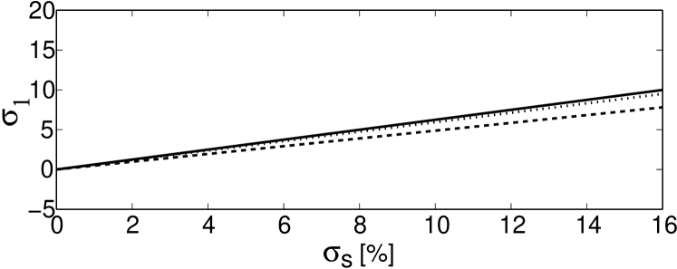
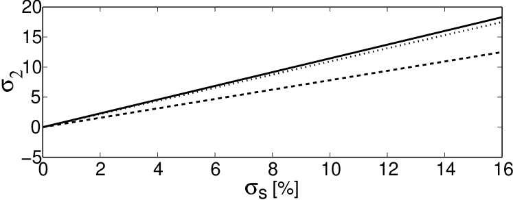
It is expected that the magnetic characteristics of each of the spacecraft units will not change due to launch stresses. However, the measurements taken onground may not be accurate enough to represent the real magnetic inflight characteristics of these units. For instance, some units would be missing during the onground measurement campaign or some others can change their magnetic characteristics during the lifetime of the mission or, finally, it could be as well that the system operation cannot be measured onground accurately. For all these reasons the predictions of the neural network may be biased. Hence, it is important to assess the robustness of the predictions of the neural network in front of changes in the magnetic dipoles of the electronic boxes. To do so we have adopted the following procedure. We varied randomly each of the components of the magnetic field of all the sources of magnetic field according to Gaussian distributions. The width of such Gaussians, , is our free parameter and corresponds to a given percentage of deviation of the specific component with respect to that of the training set. In this way we can simulate a difference between flight and ground data in a simple and realistic manner.
The results obtained using this procedure are shown in figure 4, where we show the standard deviation of the probability density function of the estimation of the three components of the magnetic field interpolated using the trained neural network as a function of the width of the Gaussians. As can be seen in this figure, the error of the estimate increases linearly for increasing widths of the Gaussian. Nevertheless, our simulations show that offsets of per component in each of the magnetic sources result in a global error of the estimate of for the magnetic field and of only for the gradient at the positions of the test masses, a very interesting result. Thus, we conclude that our interpolation scheme is fairly robust in front of small differences in the flight-ground data configuration.
4 Offsets in the magnetometers
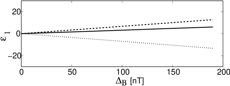
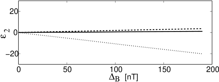
It has been shown recently that the magnetometers readings may suffer from an unpredictable offsets bib:magOffset due to launch stresses. In particular, this offset is most problably due to temperature changes during launch, and varies from nT to several nT. This, of course, may have important consequences in the estimate of the magnetic field at the positions of the magnetometers, as the interpolating algorithm presented here largely depends on the reading of the magnetometers.
To assess the robustness of the interpolation scheme to the offsets in the readings of the magnetometers we have simulated a random vector of offsets (a 12 valued-vector, 1 offset for each of the 12 magnetic channels), according to a Gaussian distribution of width . This offset vector has been added to the inflight readings when performing the assessment of the results output by the interpolation network. Several simulations have been performed varying from 1 nT to 200 nT. The results are shown in figure 5. As can be observed, the errors in magnetic field estimation are below 10% up to an offset level at the magnetomters of 80 nT — which is one order of magnitude larger than the offset observed in other space missions bib:magOffset . Consequently, we conclude that the magnetic data analysis of the mission will not be appreciably affected by the possible offset of the magnetometers readings.
5 Precision of the position of the magnetometers
Another aspect which may also be relevant for the determination of the magnetic field and gradients at the positions of the test masses is the uncertainty in the location of the heads of the magnetometers. Actually, the neural network is trained with the nominal position of the magnetometers, and the inflight training will be done with these nominal values. The uncertainty in these values may represent an important source of error because the neural network learns from the geometrical distances between the test masses and the magnetometers — see table 3.
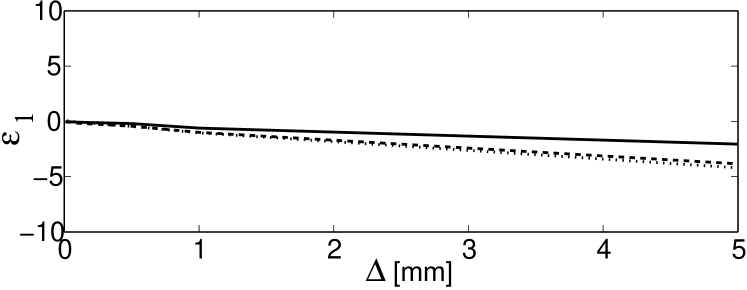

The onboard tri-axial magnetometers will be four TFM100G4-S. These are fluxgate magnetometers built by Billingsley. By construction, these magnetometers consist of three different magnetic sensors, along the -, - and -directions. For each of these axes, the fluxgate magnetometer consists of a sensing (secondary) coil surrounding an inner drive (primary) coil around permeable core material. Due to the large size of the head of these low-noise magnetometers, the spatial resolution in each of the directions is mm. On the other hand, the coils of the magnetometers have an orthogonality better than . This angular error may be transformed to a linear uncertainty by multiplying by the longest distance inside the magnetometer caging, mm, resulting in an uncertainty of mm. Finally, the exact placement of the satellite units onto the satellite walls may be unprecise. It is estimated that the mechanical precision will be on the order of the m, and therefore it will be considered negligible in this analysis. The overall spatial uncertainty of the sensing position of the magnetometers can be computed by adding in quadrature the different contributions, and turns out to be mm. In view of these conundrums we performed an additional set of simulations in which the positions of the magnetometers where randomly changed within 5 mm. We then computed the error in the estimate of the interpolating neural network. The results are shown in figure 6. Clearly, the neural network outputs a mean error in interpolation below 6% if the mechanical uncertainty lies below 4.3 mm, which is the worst case expected in the mission. Therefore, the neural network is expected to be very robust to this kind of uncontrollabale situations.
6 Varying environmental conditions
As can be seen in Eq. (2), there is a non-linear dependence of the force on the magnetic field. This means that the acceleration depends on the temporal variations of the magnetic field and its gradient. Specifically, a coupling of the value of the magnetic field with the variations of its gradient (and viceversa) exists. In the previous sections we have shown that our neural network interpolating algorithm correctly retrieves the values of the magnetic field and its gradient at the positions of the test masses when they are assumed to do not vary with time. However, these quantities are expected to be subject to small low-frequency fluctuations. Thus, we need to assess if our method is able to correctly follow a slow drift of the magnetic field and its gradient.
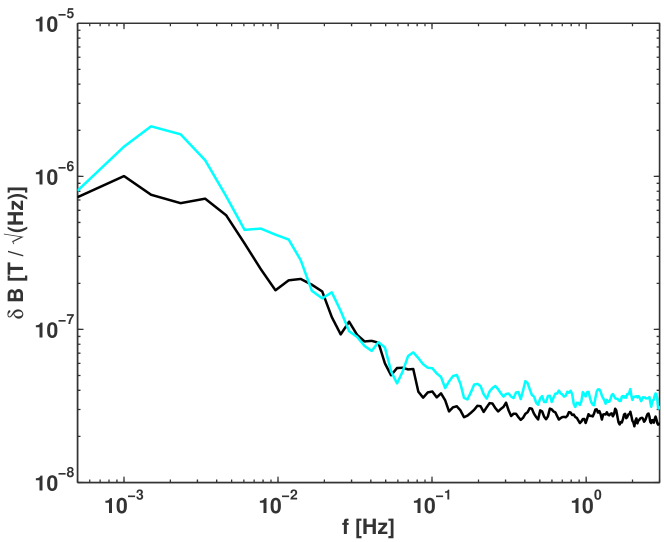
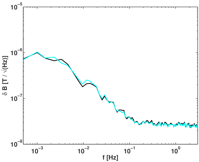
As previously mentioned, the magnetic field inside the LCA is a consequence of the electronic subsystems present inside the spacecraft. Almost all operational amplifiers (the most important source of noise of the electronics processing chain of each unit) are subject to a noise around 0.1 Hz or higher frequencies. Magnetic tests of every unit have not yet been performed, but it is foreseen that the spectrum of fluctuations of the magnetic field at the position of the test masses will be very similar to the noise spectrum of the amplifiers. In particular, it is expected that the spectrum will have a branch below a roll-off frequency of 0.1 Hz, and a white noise branch extending up to 10 Hz. The predicted spectrum, which has been obtained assuming a worst-case scenario — that is, assuming an amplitude A m at 0.1 Hz — is shown in figure 7. As it will be shown below, one of the direct consequences of including the fluctuations given by the noise spectrum of figure 7 is the presence of low-frequency variations of up to 300 nT for each of the three magnetic components. These fluctuations may cause important errors in the magnetic field estimation if not considered in the training process.
Neural networks can be classified into dynamic and static categories. Static networks have no feedback elements and, consequently, contain no delays. Thus, the output is calculated directly from the input (and only the current input) through feedforward connections bib:kecman . The training of static networks is performed with the well known and efficient backpropagation algorithm, as described in section 2.2. In dynamic networks, the output depends not only on the current input to the network, but also on its previous inputs and outputs bib:dreyfus ; bib:kecman . Thus, for our case one might quite naturally think that we should be forced to choose a dynamic neural network. Nevertheless, as shown in section 2.5, the most important feature of our interpolation scheme is the ability of the neural network to learn the underlying structures of the magnetic field inside the LCA. Since training a dynamic network is hard task and, moreover, the learning rate is usually very slow it is worth exploring the possibility of using instead a static network with an adequate training procedure adapted to this new scenario. In other words, we have to let know the network during the training process that a drift occurs. To do this we use a simple and effective training procedure. We first generate 10 different time series using uncorrelated white noise realizations. We then compute the dynamic range of the magnetic field for each of these realizations. Of these time series we select those five which have the widest dynamical range, and we concatenate them. These 5 time series are then used to train the network.
| Constant B | Fluctuating B | |||
|---|---|---|---|---|
| 2.68 | 3.28 | 8.75 | 14.75 | |
| 2.71 | 3.27 | 4.86 | 8.46 | |
| 3.15 | 3.82 | 2.92 | 13.16 | |
| 2.13 | 3.15 | 5.85 | 16.30 | |
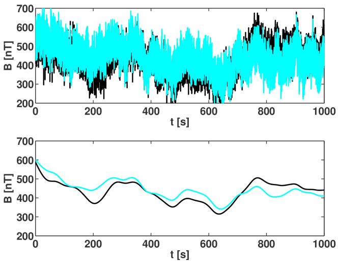
With this new training technique the interpolation results are remarkably good. To illustrate the goodness of our interpolation procedure in the top panel of figure 8 we show the temporal evolution of the fluctuating magnetic field for test mass 1 (black line) and the interpolated result obtained using the neural network trained with the fluctating examples (cyan line). As can be seen, although there are some differences, the result of the interpolation closely resembles the actual magnetic field. This can be better appreciated when both signals are filtered at 10 mHz using a low-pass filter (bottom panel of this figure). Clearly, the interpolated magnetic field follows very closely the real magnetic field. Moreover, the spectrum of the interpolated magnetic field is very similar to that of figure 7. This is borne out from figure 9, in which we compare both spectra. Clearly, the interpolated spectrum (cyan line) follows very closely the real one (black line), indicating that the neural network correctly describes the physical properties of the varying magnetic field. The only remarkable difference when a fluctuating magnetic field is analyzed is that in this case the neural network performs slightly worse. This can be seen in table 4, where we show the standard deviations of the estimates for both a constant magnetic field and a fluctuating one, for all the field components and its modulus and for both test mass 1 () and test mass 2 (). As can be seen, the estimation errors are larger for a fluctuating magnetic field, as it should be expected, but do not increase dramatically.
7 Summary and conclusions
LISA Pathfinder is a very challenging space mission, since it will test in flight many novel (and critical) technologies which are needed to satisfactorily put in orbit the first space-borne gravitational wave detector. More specifically, this mission will measure and control very accurately the motion of two test masses in almost perfect gravitational free-fall. To do this, the diagnostic system of LISA Pathfinder will monitor with unprecedented accuracy the disturbances of the motion of the test masses. An essential part of this subsystem is the magnetic diagnostics subsystem, which will be in charge of measuring the magnetic noise. To this end, this subsystem has four tri-axial magnetometers, which due to design constraints are placed far from the positions of the test masses. Thus, measuring the magnetic field at these positions is not an easy task. To overcome this problem a novel approach in which neural networks were used was recently proposed bib:myPaper . The initial results obtained using this technique were encouraging but a full assessment of its reliability was still lacking.
Accordingly, we have studied how different alternatives for the architecture of the neural network affect the precision of the interpolation of the magnetic field and its gradients at the position of the test masses. We have performed a study of the underlying structures of the neural network and we have found that the ability of our interpolating scheme to recover the correct values of the magnetic field and gradients at the positions of the test masses is due to the fact that the neural network is able to learn from the readings of the magnetometers which are closest to the corresponding test mass, and that the most important contribution for each component field comes from the corresponding magnetomer reading. We have also found that the number of neurons in the hidden layer originally proposed is the optimal one, and that a larger number of neurons in this layer does not improve the quality of the interpolation. Also, the results are not sensitive to the choice of the transfer function, and consequently the simplest choice, a linear transfer function, is the best option. Finally, we have also found that the optimal number of hidden layers is just one.
We have also discussed how the neural network must be trained with real data. In particular, we stress the importance of finding a training process adequate to the set of data the magnetometers will deliver in flight. This underlines the need to characterize on ground to our best ability the magnetic field distribution across the LCA for as many as possible foreseeable working conditions. This information will be obtained from the Magnetic Test Campaign, to be performed during 2011. Reliable information on the magnetic characteristics is essential for a meaningful assessment of magnetic noise in the LTP, and may lead to model various networks for different magnetic configurations. Our results indicate that when typical variations in the magnitudes of the magnetic dipoles of the electronic units are fed into our neural network algorithm the quality of the estimates of the magnetic field and its gradients degrade linearly with increasing departures from the onground measurement, although the measurements of the magnetic field degrade faster than those of the gradient components. However, the quality of the estimates does not degrade dramatically.
We have also studied which would be the effect in the on-flight measurements of an offset in the readings of magnetometers caused by temperature changes during launch, and we have found that, for typical offsets, the interpolating algorithm works reasonably well. The same can be said about the uncertainty in the position of the head of the magnetometers.
Finally, we have also assessed the accuracy of the magnetic field interpolation when a low-frequency drift of the magnetic characteristics is present, concluding that with an appropriate training procedure, good results are obtained. Thus, we conclude that the neural network interpolating algorithm is robust enough to obtain a good estimate of the magnetic field at the positions of the test masses under most circumstances.
Acknowledgments
This work was partially supported by MCINN grants ESP2004-01647 and AYA08–04211–C02–01. Part of this work was also supported by the AGAUR. We thank our anonymous referee, whose comments helped to improve the manuscript.
References
- (1) A. Hammesfahr et al., LISA Final Technical Report, ESTEC Contract 13631/99/NL/MS Report LI-RP-DS-009 (2000)
- (2) W.M. Folkner, F. Hechler, T.H. Sweetser, M.A. Vincent, & P.L. Bender, Class. & Quantum Grav., 14, 1405 (1997)
- (3) http://list.caltech.edu/doku.php?id=start
- (4) S. Anza et al., Class. & Quantum Grav., 22, 125 (2005)
- (5) The LISA International Team, ESA-NASA Report LISA-SCRD-Iss5-Rev1 (2008)
- (6) J. Sanjuán et al., Rev. of Sci. Inst., 79, 084503 (2008)
- (7) S. Vitale, Science requirements and top-level architecture definition for the LISA Technology Package (LTP) on board LISA Pathfinder (SMART-2), Report no. LTPA-UTN-ScRD-Iss003-Rev1 (2005)
- (8) P. Canizares et al., Class. & Quantum Grav., 26, 094005 (2009)
- (9) M. Diaz-Aguilo, E. García–Berro & A. Lobo, Class. & Quantum Grav., 27, 035005 (2010)
- (10) V. Kecman, Learning and soft computing, MIT Press, 1st edition (2001)
- (11) R.J. Bullen, D. Cornford, & I.T. Nabney, Neural Networks, 16, 419 (2003)
- (12) D.G. Loyola, Neural Networks, 19, 168 (2006)
- (13) R. Reed, IEEE Trans. on Neural Networks, 4, 740 (1993)
- (14) B. Amirikian, & H. Nishimura, in Proc. of the Second International Symposium on Intelligent Information Technology Applications (2008)
- (15) C. Schittenkopf, G. Deco, & W. Brauer, Neural Networks, 10, 505 (1997)
- (16) G. Dreyfus, Neural Networks: Methodology and Applications, Springer Verlag, 2nd edition (2005)
- (17) F. Primdahl, T. Risbo, J. Merayo, P. Brauer, & L. Toffner-Clausen, Meas. Sci. & Technology, 17, 1563 (2006)