Excitation spectrum for an inhomogeneously dipole-field-coupled superconducting qubit chain

Abstract

When a chain of $N$ superconducting qubits couples to a coplanar resonator in a cavity, each of the qubits experiences a different dipole-field coupling strength due to the waveform of the cavity field. We find that this inhomogeneous coupling leads to a dependence of the qubit chain’s ladder operators on the qubit-interspacing $l$. Varying the spacing $l$ changes the transition amplitudes between the angular momentum levels. We derive an exact diagonalization of the general $N$-qubit Hamiltonian and, through the $N=4$ case, demonstrate how the $l$-dependent operators lead to a denser one-excitation spectrum and a probability redistribution of the eigenstates. Moreover, we show that the variation of $l$ between its two limiting values coincides with the crossover between Frenkel- and Wannier-type excitons in the superconducting qubit chain.

I Introduction

Superconducting quantum circuits have attracted considerable attention because of their capabilities (i) to demonstrate macroscopically the basic interaction of one “atom” and one photon in a cavity (e.g., jqyou03 ; blais04 ), (ii) to serve as a platfrom for testing many quantum optical phenomena (e.g., hauss08 ; ian10 ; shevchenko10 ; jqyou11 ; wilson11 ), as well as (iii) to show its potential as a basis for quantum information processing (e.g., jqyou05 ; yxliu06 ; hemler09 ; buluta11 ).

While research on single-qubit interactions are more common, many recent articles also studied multi-qubit interactions. Superconducting circuits with such interactions are also known as quantum metamaterials rakhmanov08 . To be precise, the circuit system we consider here consists of a chain of $N$ superconducting two-level qubits coupled to a photon mode in a superconducting coplanar waveguide resonator. Compared to the single-qubit version, it can manifest even more quantum phenomena, including plasma waves savelev10 , controllable collective dressed states fink09 , and quantum phase transitions wang07 ; lambert09 ; nataf10 ; tian10 . It also promises potential for various applications, including quantum simulators buluta09 and quantum memories diniz11 .

Theoretical studies of multi-qubit interactions with a photon often employ the Dicke model dicke54 , where the Pauli operators are summed and transformed into a bosonic operator. In this approach, the chain of qubits is treated collectively as an atomic ensemble and the excited qubits are collectively regarded as one exciton mode. This theoretical simplification proves adequate when (i) the number of excitations in the system is low (in the so-called “one-photon” processes) and (ii) the number of qubits is large enough such that the interspacing $L_{\mathrm{q}}$ between neighboring qubits can be ignored compared to the photon wavelength $L_{\mathrm{p}}$ in the resonator (i.e., the qubits can be regarded as a continuum).

However, the question of how excitations arise in superconducting metamaterials when these two conditions are not met remains unanswered. In a realistic setting for a superconducting circuit, the number $N$ of qubits present can range from one to, say, 10, but $N$ would not be as large as the number of atoms we usually have for an alkaline atomic ensemble in an optical microcavity, which is typically greater than $10^{5}$. Therefore, the Dicke model, which treats $N\to\infty$, does not apply well to the case of multi-qubit superconducting circuits with $N\leq 10$.

When a chain of superconducting circuit qubits is arranged as a one-dimensional array (i.e., a superconducting qubit chain or SQC), each qubit is inhomogeneously coupled to the circuit photon mode. In other words, each qubit has a different coupling strength to the traversing photon field. This occurs naturally since, unlike its optical cavity QED counterpart, the photon wavelength $L_{\mathrm{p}}$ is comparable to the qubit interspacing $L_{\mathrm{q}}$ in a superconducting circuit. The coupling strength thus depends on the position of the qubit relative to the photon waveform. The effect of the varying coupling strength becomes even more obvious if multi-mode couplings are taken into consideration. For example, the qubits on the antinodes of the waveform will couple most strongly, whereas those on the nodes will not couple.

The first step to understand and characterize this inhomogeneously-coupled system (the aim of this article) is to obtain the energy spectrum of the collective excitation mode in the chain of qubits and to compare it with that of the Dicke model. We find that the inhomogeneity of the couplings incurs an algebraic deformation of the Pauli operators of the qubits polychron90 ; rocek91 ; delbecq93 ; bonatsos93 . We quantify this deformation through a “deformation factor,” which is a function of the relative spacing $l=2L_{\mathrm{q}}/L_{\mathrm{p}}$, and characterize the amount the inhomogeneous system deviates from the homogeneous case. The deformation factor modifies the spin operators of the collective qubit chain. Consequently, the excitation spectrum will not only be a function of the eigenenergy of the photon mode and the qubit level spacing, but is also highly related to the deformation factor and hence the relative spacing $l$.

Note that when atoms are confined to a cavity, the magnetic or laser field that is exerted on them is uniform. The strength of the interaction can be uniformly increased or decreased according to the density of the atoms. This macroscopic viewpoint does not differentiate between the identities of the atoms. However, for circuit QED, the identities of the qubits are partially differentiated since the qubits can be categorized according to the values of their coupling strength to the photon mode. This partial differentiation has made understanding the inhomogeneous system a many-body physics question.

Our deformation algebraic approach here is a statistical approximation method that can be regarded as finding the average contribution of the coupling strength given by the SQC as a whole. In the end, the characterization (the excitation spectrum) of the SQC as an inhomogeneous system is not parametrized by the individual qubits, but by the relative spacing $l$. In other words, the spacing $l$ is one extra degree of freedom peculiar to the inhomogeneous SQC, not seen in a homogeneous optical cavity.

We will first introduce the model and derive the deformation factor in Sec. II. With the deformation factor, new operation rules for the spin angular momentum operators are found by solving a difference equation in Sec. III. The general energy spectrum for $n$-qubit SQC is given in Sec. IV. We also derive in Sec. IV a one-excitation spectrum for a 4-qubit SQC as a nontrivial case to show the effects of the inhomogeneity. Namely, the energy splittings between the eigenstates of the deformed coupling case shrink, while the probability amplitudes of the eigenstates are redistributed such that higher-photon occupations are favored.

In the final Sec. V, we will consider how the collective excitations on the SQC would emulate the excitons in atomic lattices. In one limit, it becomes a Wannier-type exciton Mahan , where the wave function of the excited level is localized on a single atom. In the opposite limit, it emulates a Frenkel-type exciton, which has an extended wave function across multiple atoms. Changing the degree of freedom $l$ lets the emulated exciton undergo a crossover between these two types of excitons. This crossover depends on a $(2N-1)$-th order trigonometric equation, whose solution corresponds to the asymptotic turning point from the deformed (inhomogeneously-coupled) SQC to the undeformed (homogeneously-coupled) SQC.

II Inhomogeneous coupling model

II.1 Inhomogeneous coupling

For a finite number $N$ of spins in the SQC, the problem discussed here is similar to the Tavis-Cummings (TC) model tavis68 ; swain72 , where all the spins are grouped into a total “large” spin. However, the exactly solvable TC model applies only when the coupling is homogeneous and when the eigenfrequencies between the qubits and the photon mode are equal. When the coupling is inhomogeneous, the large spin does not obey the usual commutation relations of the Pauli matrices, which the TC-model assumes.

The new commutation relations of the large spin introduced by the inhomogeneity are pertinent to the deformed SU(2) Lie algebras. From these algebraic structures, we can establish a deformed dipole-field coupling model, of which the TC model is a special case. In the following discussion, we consider the typical case where the inter-qubit spacing is uniform. The coupling strength of each qubit to the photon field can, therefore, be written as a cosine function of a phase factor which is determined by the position $jl$ of the $j$-th qubit, where $j$ is the reduced coordinate and $l$ is the relative spacing introduced above.

The situation is illustrated in Fig. 1(a). A chain of qubits is sandwiched between the superconducting coplanar resonator and a superconducting ground strip. The photon mode providing different potential energies on the spins is shown by the red sinusoidal curve.

We use the operators $\{\sigma_{j,z}\}$ to denote Josephson junction qubits, and $\{a,a^{\dagger}\}$ to denote the operators for the single-photon mode. With the wave vector being the reciprocal of the photon field wavelength on the one-dimensional lattice, $k=2\pi/L_{\mathrm{p}}$, the dipole-field coupling is of the form $\sigma_{j,x}(a\cos(j\pi l)+\mathrm{h.c.})$. Under the rotating wave approximation, the Hamiltonian can be written as ($\hbar=c=1$)

$$H=\omega_{\mathrm{q}}\sum_{j=0}^{N-1}\sigma_{j,z}+\omega_{0}a^{\dagger}a+\eta\sum_{j=0}^{N-1}\cos(j\pi l)\left[\sigma_{j,+}a+\sigma_{j,-}a^{\dagger}\right]$$ (1)

where $\omega_{\mathrm{q}}$ is the eigenenergy of the spins, $\omega_{0}$ the mode frequency of the photon, and $\eta$ the coupling amplitude.

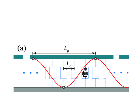
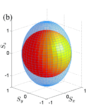
Figure 1: (Color online) (a) Schematic diagram of an SQC with spacing $l=1/3$. The upper strip represents a coplanar resonator whose potential waveform of wavelength $L_{\mathrm{p}}$ is drawn as a sinusoidal curve, while the lower one represents a ground strip. The rectangles between the strips are qubits with interspacing $L_{\mathrm{q}}$. The gray dots on the curve indicate the anti-nodes of the waveform. (b) The elongation effect on the large spin due to inhomogeneous coupling. The ellipsoid shows a case of deformation $R_{N,l}=0.5$. The unit sphere shows the spin under the usual homogeneous coupling.

To diagonalize the Hamiltonian in Eq. (1), we introduce the “large spin” operators: the magnetic moment or $z$-direction collective spin operator

$$S_{z}=\sum_{j=0}^{N-1}\sigma_{j,z},$$ (2)

which is no different from the homogeneous case, and the paired raising and lowering operators

$$S_{+} = \sum_{j=0}^{N-1}\sigma_{j,+}\cos(j\pi l)$$ (3)

$$S_{-} = \sum_{j=0}^{N-1}\sigma_{j,-}\cos(j\pi l)$$ (4)

which have the special sinusoidal dependence on $l$ due to the inhomogeneity. The commutator of the paired ladder operators no longer equals to $2S_{z}$ but has an additional term due to the cosine coefficients, i.e., $[S_{+},S_{-}]=2\Sigma_{z}$ with

$$\Sigma_{z}=S_{z}+\sum_{j=0}^{N-1}\sin[j\pi(1+l)]\sin[j\pi(1-l)]\sigma_{j,z}.$$ (5)

The detailed derivation is shown in Appendix A.1. Note that in the usual circuit QED system blais04 , where only one spin is placed at midway, the spacing $l$ equals to 2, for which the latter term in $\Sigma_{z}$ vanishes. This is the limiting case which corresponds to the Wannier type of excitation, where the set of spin operators retains the usual structure of an undeformed SU(2) algebra.

II.2 Deformed algebraic structure

When the second term of $\Sigma_{z}$ does not vanish, the algebraic structure is called deformed polychron90 ; rocek91 ; delbecq93 ; bonatsos93 . In order to quantify the deformation, the commutator of the ladder operators needs to be expressed as a function of $S_{z}$, i.e., $\Sigma_{z}=f(S_{z})$. To find this function $f$, we consider an underlying manifold, on which there is a local point, say the origin 0, where we define a tangent space with the Pauli $z$-matrices $\{\sigma_{j,z}\}$ being its basis vectors, since these matrices are linearly independent. The operator $S_{z}$, defined above with uniform coefficients, can be deemed a vector in this tangent space; the operator $\Sigma_{z}$ is then another vector dependent on the parameter $l$ and is a deviation or deformation from $S_{z}$. Thus, the first-order approximation of $\Sigma_{z}$ with respect to $S_{z}$ is its projection onto the vector $S_{z}$. That is, since the cosine coefficients are bounded, we can use their Hilbert-Schmidt norm

$$\left\langle\Sigma_{z},S_{z}\right\rangle=\mathrm{tr}\left(\Sigma_{z}^{\ast}S_{z}\right)=N+\sum_{j=0}^{N-1}\cos(2j\pi l)$$ (6)

and the Schmidt decomposition reed_simon to write $\Sigma_{z}=R_{N,l}S_{z}$ as a deformation of the original $z$-spin operator where

$$R_{N,l}=\frac{1}{4N}\left\{2N+1+\frac{\sin[(2N-1)\pi l]}{\sin(\pi l)}\right\}$$ (7)

is the deformation factor (Cf. Appendix A.2 for this derivation). The commutator of the ladder operators can now be expressed as

$$[S_{+},S_{-}]=2R_{N,l}S_{z},$$ (8)

where $R_{N,l}$ has a limiting value of one when $l\to 0$ or $l\to\infty$, for which the usual structure used in the TC model is retained.

Since the deformation factor $R_{N,l}$ does not affect the commutation relations between the ladder operators and the $z$-spin, the large-spin operators $\{S_{z},S_{+},S_{-}\}$ form a specific deformed algebra polychron90 ; rocek91 and not the more general type delbecq93 . The Casimir operator

$$C=S_{-}S_{+}+h(S_{z})$$ (9)

of the algebra, which equals to the undeformed spin momentum square, $S^{2}=S_{x}^{2}+S_{y}^{2}+S_{z}^{2}$, for the homogeneous coupling case, is accordingly deformed. Through solving a recursive relation (Cf. Appendix A.3 for details), we find $h(S_{z})=R_{N,l}(S_{z}^{2}+S_{z})$ and hence

$$C=S_{x}^{2}+S_{y}^{2}+R_{N,l}S_{z}^{2},$$ (10)

which shows that the spin momentum is reduced along the $z$-direction:

$$S^{2}=S_{x}^{2}+S_{y}^{2}+R_{N,l}S_{z}^{2}.$$ (11)

To visualize this reduction of the spin momentum, we can take a unit value for the spin moment and let the Casimir operator be represented by a unit sphere in 3-dimensional space for the undeformed case. With $R_{N,l}\leq 1$, the deformation would be an elongation of the unit sphere, along the $z$-axis, to an ellipsoid, while the $x$- and $y$-semi-minor axes remain unchanged, as shown in Fig. 1(b).

III Operation rules

If we consider the unit sphere of Fig. 1(b) as a Bloch sphere on which the large spin prescribes its $N$ levels, its elongation due to deformation will accordingly modify the transitions between the levels. Since the spin-up and the spin-down momenta do not change, which are still $\omega_{\mathrm{q}}N/2$ and $-\omega_{\mathrm{q}}N/2$, the narrow part of the ellipsoid effectively squeezes the transition probabilities.

More precisely, we consider an arbitrary eigenstate $\left|r,m\right\rangle$, for which

$$S_{z}\left|r,m\right\rangle = m\left|r,m\right\rangle$$ (12)

$$S^{2}\left|r,m\right\rangle = r(r+1)\left|r,m\right\rangle.$$ (13)

The ladder operators result in an $(r,m)$-dependent off-diagonal matrix element $\alpha_{m}^{(r)}$, i.e.,

$$S_{+}\left|r,m\right\rangle = \alpha_{m}^{(r)}\left|r,m+1\right\rangle$$ (14)

$$S_{-}\left|r,m\right\rangle = \alpha_{m-1}^{(r)}\left|r,m-1\right\rangle$$ (15)

By examining the diagonal elements of the commutator of the ladder operators, we find a difference equation $(\alpha_{m}^{(r)})^{2}-(\alpha_{m-1}^{(r)})^{2}=-2mR_{N,l}$. With the value $\alpha_{-r}^{(r)}=0$, the equation can be solved to give the deformed off-diagonal matrix elements or transition probabilities for the ladder operators

$$\alpha_{m}^{(r)}=\sqrt{R_{N,l}(r-m)(r+m+1)}.$$ (16)

See Appendix B for its derivation.

Geometrically speaking, the deformation process is a homeomorphism with a redefined metric $g=(1,1,R_{N,l})$. Since $R_{N,l}\leq 1$, the metric norm is less than unity. The deformation does not affect the level spacings of the magnetic moment $S_{z}$: the number $m$ still takes $(2r+1)$ values (i.e., the ellipsoid is homeomorphic to the sphere). But the transition amplitudes to traverse the sphere decrease: if we start with a spin-up state $\left|r,r\right\rangle$ and finish with a spin-down state $\left|r,-r\right\rangle$, then all iterations with $S_{-}\left|r,m\right\rangle=\alpha_{m-1}^{(r)}\left|r,m-1\right\rangle$ have $\alpha_{m}^{(r)}$ smaller than the original $\bar{\alpha}_{m}^{(r)}=\sqrt{(r-m)(r+m+1)}$ (i.e., the ellipsoid is not isometric to the sphere).

The deformation factor expressed in Eq. (7) is an oscillating function of $l$, where the sine in the numerator determines the period of oscillation and the sine in the denominator determines the period of the envelope. Therefore, the spin angular momentum of the SQC would be oscillating between the unit sphere and the ellipsoid, depending on the qubit spacing $l$. The plot of $R_{N,l}$ in Fig. 2(a) for an SQC of $N=30$ qubits shows a typical case with envelop of period 1 and local minimum of $0.4$. The function $h(S_{z})$ associated with this deformation factor is a parabola of the magnetic moment $S_{z}$. For a nontrivial deformation $R_{N,l}<1$, this parabola flattens and the spin levels become denser. The curvature of the parabola decreases while its minimum value $-R_{N,l}/4$ increases. As shown in Fig. 2(b), the black (gray) arrow indicates the spin level $r=1/2$ for the deformed $R_{N,l}=0.4$ (undeformed $R_{N,l}=1$) case of SQC. So varying $l$ makes the curve $h(S_{z})$ oscillate between the boldened curves that correspond to $R_{N,l}=0.4$ and $R_{N,l}=1$, respectively. We can also observe that the level splittings are reduced, reflecting the elongated structure of the Bloch sphere in Fig. 1(b) and the modified operation rule of Eq. (16).

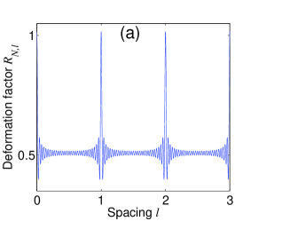
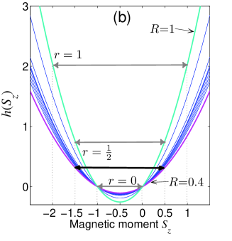
Figure 2: (Color online) (a) The deformation factor $R_{N,l}|_{N=30}$, as an oscillating function of the qubit spacing $l$. (b) Plot of the function $h(S_{z})$ for various values of $R_{N,l}$. The top and bottom boldened curves correspond to $R_{N,l}=1$ and $0.4$, respectively. The gray-shaded double-arrows indicate three spin levels of the undeformed SQC, while the black arrows show the $r=1/2$ level of the deformed case.

IV Deformed spectrum

Equipped with the modified operation rules, we can diagonalize the Hamiltonian in Eq. (1). First, we split the Hamiltonian into two parts

$$H_{0} = \omega_{0}(S_{z}+a^{\dagger}a),$$ (17)

$$H_{1} = \tilde{\omega}_{0}a^{\dagger}a+\eta(S_{+}a+S_{-}a^{\dagger}).$$ (18)

Let $u$ be the number of total excitations and hence the eigenvalue of $H_{0}$. Let $n$ be the number of photons in the system such that the SQC magnetic moment is $m=u-n$. Let $\nu$ be the eigenvalue of the interaction part $H_{1}$, where $\tilde{\omega}_{0}=\omega_{0}-\omega_{\mathrm{q}}$.

The eigenvector of the Hamiltonian can then be expanded as a superposition of different configurations of photon number and spin states:

$$\left|u,r\right\rangle=\sum_{n}c_{n}\left|n;r,u-n\right\rangle.$$ (19)

The expansion coefficients $c_{n}$ satisfy a recursive relation swain72 :

$$c_{n+1}\sqrt{n+1}\alpha_{u-(n+1)}^{(r)}-c_{n}\tilde{v}_{n}+c_{n-1}\sqrt{n}\alpha_{u-n}^{(r)}=0$$ (20)

where $\tilde{v}_{n}=(v-\tilde{\omega}_{0}n)/\eta$.

The solution reads

$$c_{n}=\sum_{p=0}^{\lfloor n/2\rfloor}(-1)^{p}\left(R_{N,l}\right)^{p-n/2}\mathscr{C}_{n,p}.$$ (21)

$\mathscr{C}_{n,p}$ can be regarded as a probability amplitude contribution to the $n$-photon state from a set of corresponding qubit chain states indexed by $p$:

$$\mathscr{C}_{n,p}=\frac{P_{n}}{\sqrt{n!}}\underset{\langle j_{1}\dots j_{k}\dots j_{\lfloor n/2\rfloor}\rangle}{\sum\cdots\sum}\prod_{k=1}^{p}\frac{(j_{k}+1)}{\tilde{v}_{j_{k}}\tilde{v}_{j_{k}+1}}\left[\bar{\alpha}_{u-(j_{k}+1)}^{(r)}\right]^{2}$$ (22)

where $P_{n}=\prod_{j=0}^{n-1}\tilde{v}_{j}/\bar{\alpha}_{u-(j+1)}^{(r)}$ and $\left\langle j_{1}\dots j_{k}\dots j_{\lfloor n/2\rfloor}\right\rangle$ represents an index set of descending order $\{\forall k<l:0\leq j_{l}\leq j_{k}-2;0\leq j_{1}\leq n-2\}$. We can see from Eq. (21) that the operation rules discussed in the preceding paragraphs have made the probability amplitudes deformation-dependent, thus $l$-dependent. This will consequently lead to a redistribution of probabilities for different photon states. See Appendix C.1 for the derivation of these coefficients $\mathscr{C}_{n,p}$.

Table 1: Configurations $\left|n;r,m\right\rangle$ and probability amplitudes $c_{n}$ for the one-excitation spectrum of an SQC with $N=4$ qubits and spacing $l=2/3$. Each $\circ$ indicates one photon while $\uparrow$ or $\downarrow$ denotes the spin state of each qubit. Here, $\tilde{v}_{n}=(v-\tilde{\omega}_{0}n)/\eta$. 

$\begin{array}[]{c}u=1\\ r=2\end{array}$	$\left\{\begin{array}[]{c}n=0\\ m=1\end{array}\right.$	$\left\{\begin{array}[]{c}n=1\\ m=0\end{array}\right.$	$\left\{\begin{array}[]{c}n=2\\ m=-1\end{array}\right.$	$\left\{\begin{array}[]{c}n=3\\ m=-2\end{array}\right.$
photon spin config.	$\begin{array}[t]{c}-\\ \downarrow\uparrow\uparrow\uparrow\\ \uparrow\downarrow\uparrow\uparrow\\ \uparrow\uparrow\downarrow\uparrow\\ \uparrow\uparrow\uparrow\downarrow\end{array}$	$\begin{array}[t]{c}\circ\\ \uparrow\uparrow\downarrow\downarrow,\downarrow\downarrow\uparrow\uparrow\\ \uparrow\downarrow\downarrow\uparrow,\downarrow\uparrow\uparrow\downarrow\\ \uparrow\downarrow\uparrow\downarrow,\downarrow\uparrow\downarrow\uparrow\end{array}$	$\begin{array}[t]{c}\circ\circ\\ \uparrow\downarrow\downarrow\downarrow\\ \downarrow\uparrow\downarrow\downarrow\\ \downarrow\downarrow\uparrow\downarrow\\ \downarrow\downarrow\downarrow\uparrow\end{array}$	$\begin{array}[t]{c}\circ\circ\circ\\ \downarrow\downarrow\downarrow\downarrow\end{array}$
$c_{n}$	1	$\frac{\tilde{v}_{0}}{\sqrt{6R}}$	$\frac{\tilde{v}_{0}\tilde{v}_{1}}{6\sqrt{2}R}\negmedspace-\negthickspace\frac{1}{\sqrt{2}}$	$\frac{\tilde{v}_{0}\tilde{v}_{1}\tilde{v}_{2}}{12\sqrt{6}R^{3/2}}\negthickspace-\negthickspace\frac{\tilde{v}_{2}+2\sqrt{6}\tilde{v}_{0}}{12\sqrt{R}}$

The simplest nontrivial example of this deformation effect can be seen in Table. 1, where we consider the one-excitation ($u=1$) spectrum of a four-qubit SQC with spacing $l=2/3$. The deformation factor in this case is $R_{N,l}=5/8$. For a weakly coupled SQC with $|\tilde{\omega}_{0}|\gg\eta$, the eigenenergies for the four levels are given by (Cf. Appendix C.2 for the derivation)

$$E_{\pm,\pm}=\omega_{\mathrm{q}}+\frac{3}{2}\tilde{\omega}_{0}\pm\frac{1}{2}\left[5\tilde{\omega}_{0}^{2}\pm 4\tilde{\omega}_{0}\left(\tilde{\omega}_{0}^{2}+36R_{N,l}\eta^{2}\right)^{1/2}\right]^{1/2}.$$ (23)

For a deformation factor $R_{N,l}<1$, the splittings between these dressed levels are suppressed. In addition, if we substitute the value of $v$ into the coefficients $c_{n}$, we will find that $c_{1}$ is greater than that of the undeformed case, $c_{2}$ ($c_{3}$) increases by a greater proportion than $c_{1}$ ($c_{2}$), while $c_{0}$ remains equal to one. Therefore, the probability distribution shifts toward the end that favors states with greater number of photons and less degeneracy.

V Exciton Crossover

If the spacing $l$ is large ($L_{\mathrm{q}}\gg L_{\mathrm{p}}$), i.e., there are multiple photon wavelengths between two neighboring qubits, we can consider the excitation that the dipole-field coupling induces on a qubit to be localized on that qubit. Consequently, this type of excitation emulates the Wannier exciton on an atomic lattice. If $l$ is small ($L_{\mathrm{q}}\ll L_{\mathrm{p}}$) with a single-photon wavelength extending over all the qubits, we can consider the excitation on the SQC to be delocalized. This type of excitation emulates the Frenkel’s exciton model for molecular crystals. Note that when $l$ tends to either zero or infinity in Eq. (5), $\Sigma_{z}$ falls back to $S_{z}$ and the regular SU(2) algebra for the commutators is obtained. Thus, it is justified that in the large-$N$ limit, the low-energy excitation becomes bosonic for both Wannier and Frenkel excitons.

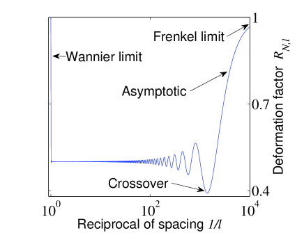
Figure 3: Semi-log plot of the deformation factor $R_{N,l}$ versus $1/l$ over one period, showing the Wannier limit on the left end and the Frenkel limit on the right end of the horizontal axis. The number of qubits is set to $N=1000$.

To determine when the emulated exciton crosses from Wannier- to Frenkel-type, we plot in Fig. 3 the deformation factor versus the reciprocal of the spacing over $10^{-4}<l<1$, where we can see the asymmetry between the left edge ($1/l\to 0$) for the Wannier limit and the right edge ($1/l\to\infty$) for the Frenkel limit. Setting $\mathrm{d}R_{N,l}/\mathrm{d}l=0$, we obtain the trigonometric equation

$$\tan[(2N-1)\pi l]=(2N-1)\tan(\pi l).$$ (24)

Transforming Eq. (24) to $U_{2N-1}(\cos\pi l)=2N\cdot T_{2N-1}(\cos\pi l)$, where $T_{2N-1}$ ($U_{2N-1}$) is the Chebyshev polynomial of the first (second) kind, we can observe that it is a $(2N-1)$-th order polynomial equation. Hence, the curve has $(2N-1)$ local extrema in exactly $(N-1)$ oscillations from the Wannier end to the asymptotic Frenkel end. Between these two limits, the excitation has various degrees of deformation and the crossover is continuous. We can regard the crossover point to be the absolute minimum before the deformation factor asymptotically approaches one. This point approaches 0 when $N\to\infty$. For the case illustrated in Fig. 3 with $N=1000$, a numerical estimation gives the crossover at $l=7.16\times 10^{-4}$, or a length of 2800 spins per photon wavelength.

VI Conclusion

We have studied the inhomogeneous coupling between a SQC and a superconducting coplanar resonator, which leads to a set of deformation-dependent operation rules of spin momentum. The modified rules correspond to tighter energy spacings and a shift of the probability distribution of spin levels. The inhomogeneous coupling also gives rise to different types (Frenkel and Wannier) of collective excitations on the SQC and the crossover between these types is determined by a polynomial equation of the qubit spacing $l$.

FN acknowledges partial support from LPS, NSA, ARO, DARPA, AFOSR, NSF grant No. 0726909, JSPSRFBR contract No. 09-02-92114, MEXT Kakenhi on Quantum Cybernetics, and Funding Program for Innovative R&D on S&T. YXL acknowledges support from the NNSFC grant No. 10975080 and 61025022.

Appendix A Derivation of the deformation factor

A.1 Commutation relation

The commutator of the ladder operators can be computed as follows

$$[S_{+},S_{-}] = \sum_{j,k=0}^{N-1}\cos(j\pi l)\cos(k\pi l)[\sigma_{j,+},\sigma_{k,-}]$$

$$= 2\sum_{j=0}^{N-1}\cos^{2}(j\pi l)\sigma_{j,z}$$

$$= S_{z}+\sum_{j=0}^{N-1}\cos(2j\pi l)\sigma_{j,z}.$$

To use a consistent notation, we write the R.H.S. as $2\Sigma_{z}$ and extract $S_{z}$ from the second term

$$2\Sigma_{z} = 2S_{z}+\sum_{j=0}^{N-1}\left[\cos(2j\pi l)-\cos(2j\pi)\right]\sigma_{j,z}$$

$$= 2S_{z}+2\sum_{j=0}^{N-1}\sin\left[j\pi(1+l)\right]\sin\left[j\pi(1-l)\right]\sigma_{j,z}$$

which gives Eq. (5).

We can also check that other commutation relations are preserved

$$[S_{z},S_{\pm}] = \sum_{j,k=0}^{N-1}\left[\sigma_{k,z},\sigma_{j,\pm}\cos(j\pi l)\right]$$

$$= \sum_{j=0}^{N}\pm\sigma_{j,\pm}\cos(j\pi l)$$

$$= \pm S_{\pm},$$

from which we conclude that the newly defined operators $\left\{S_{z},S_{+},S_{-}\right\}$ form a Polychronakos-Rocek type of deformed SU(2) algebra.

A.2 Deformation factor

First, we recognize that each qubit $\sigma_{j,z}$ has two orthonormal basis vectors $\left\{\left|e_{j}\right\rangle,\left|g_{j}\right\rangle\right\}$ for a fixed relative coordinate $j$ and hence $\left\{\left|\epsilon_{k}\right\rangle:\left|\epsilon_{k}\right\rangle\in\left\{\left|e_{j}\right\rangle,\left|g_{j}\right\rangle,j=0,\dots,N-1\right\}\right\}$ forms an orthonormal basis for the Hilbert space $\mathcal{H}$ that spans all the qubits on the chain. Then $S_{z}$ for the original spin angular momentum and $\Sigma_{z}$ for that of the inhomogeneous SQC become operators on this Hilbert space $\mathcal{H}$. Since the sinusoidal functions $\cos(j\pi l)$ are bounded, we can define the Hilbert-Schmidt inner product as

$$\left\langle\Sigma_{z},S_{z}\right\rangle = \mathrm{tr}\left(\Sigma_{z}^{\ast}S_{z}\right)=\sum_{k}^{2N}\left\langle\epsilon_{k}\right|\Sigma_{z}\cdot S_{z}\left|\epsilon_{k}\right\rangle$$

$$= \sum_{k}^{2N}\left\langle\epsilon_{k}\right|\sum_{j,l=0}^{N-1}\cos^{2}(j\pi l)\sigma_{j,z}\cdot\sigma_{l,z}\left|\epsilon_{k}\right\rangle$$

$$= \sum_{k}^{2N}\left\langle\epsilon_{k}\right|\cos^{2}(\lfloor k/2\rfloor\pi l)\sigma_{\lfloor k/2\rfloor,z}\cdot\sigma_{\lfloor k/2\rfloor,z}\left|\epsilon_{k}\right\rangle$$

$$= \sum_{k}^{2N}\cos^{2}(\lfloor k/2\rfloor\pi l)$$

$$= \sum_{j}^{N}2\cos^{2}(j\pi l)$$

which equals to Eq. (6). We can then write the approximation of $\Sigma_{z}$ as a Schmidt projection on $S_{z}$

$$\Sigma_{z} \approx \frac{\left\langle\Sigma_{z},S_{z}\right\rangle}{\left\langle S_{z},S_{z}\right\rangle}S_{z}$$

$$= \frac{N+1+\sum_{j}\cos(2j\pi l)}{2(N+1)}S_{z}$$

$$= \left[\frac{1}{2}+\frac{1}{2N}\sum_{j=0}^{N-1}\cos(2j\pi l)\right]S_{z}$$

$$= R_{N,l}S_{z}$$

where $R_{N,l}$ denotes the deformation factor. Its expression can be further simplified to

$$R_{N,l} = \frac{1}{4N}\left[2N+1-\cos(2N\pi l)+\frac{\sin(2\pi l)\sin(2N\pi l)}{1-\cos(2\pi l)}\right]$$

$$= \frac{1}{4N}\left[2N+1-\cos(2N\pi l)+\frac{\cos(\pi l)\sin(2N\pi l)}{\sin(\pi l)}\right]$$

$$= \frac{1}{4N}\left[2N+1+\frac{\sin[(2N-1)\pi l]}{\sin(\pi l)}\right]$$

where the first line is derived by comparing the real parts in a summation of exponentials.

A.3 Casimir operator

The Casimir operator for the algebra is

$$C=S_{-}S_{+}+h(S_{z})$$

where the second term satisfies a recursive relation delbecq93

$$h(S_{z})-h(S_{z}-1)=2R_{N,l}S_{z}.$$

This relation leads to a solution composed of Bernoulli polynomials

$$h(S_{z}) = R_{N,l}\left(B_{2}(-S_{z})-B_{2}\right)$$

$$= R_{N,l}\left(S_{z}^{2}+S_{z}\right)$$

where $B_{2}(-S_{z})$ is the second-order Bernoulli polynomial with the operator $S_{z}$ as variable and $B_{2}$ is the second Bernoulli number. The Casimir operator becomes then

$$C = S_{-}S_{+}+R_{N,l}\left(S_{z}^{2}+S_{z}\right)$$

$$= \frac{1}{2}(S_{+}S_{-}+S_{-}S_{+})+R_{N,l}S_{z}^{2}$$

which equals to Eq. (10) and represents a deformed total spin operator $S^{2}$.

Appendix B Deriving operation rules

Assume the eigenstate of the $z$-spin momentum operator $S_{z}$ to be $\left|r,m\right\rangle$, that is, $r(r+1)$ denotes the total spin number and $m$ the magnetic moment, for which Eqs. (12)-(13) are satisfied. Further, assume $\alpha_{m}^{(r)}$ to be the coefficients when the ladder operators are applied to the state vectors as in Eqs. (14)-(15), which is indexed by $r$ and $m$.

By applying the vector $\left|r,m\right\rangle$ to the commutation relation Eq. (8), we find

$$\left\langle r,m\right|\left[S_{+},S_{-}\right]\left|r,m\right\rangle = \left\langle r,m\right|S_{+}S_{-}-S_{-}S_{+}\left|r,m\right\rangle$$

$$= (\alpha_{m-1}^{(r)})^{2}-(\alpha_{m}^{(r)})^{2}$$

$$= \left\langle r,m\left|2R_{N,l}S_{z}\right|r,m\right\rangle$$

$$= 2R_{N,l}m.$$

Selecting the second and the fourth line, we arrive at a difference equation of $m$:

$$(\alpha_{m}^{(r)})^{2}-(\alpha_{m-1}^{(r)})^{2}=-2mR_{N,l}.$$

To solve the equation, we list out the iterations until the last entry where $\alpha_{-r-1}^{(r)}=0$ since $-r$ is the minimum value $m$ can take as the magnetic moment

$$(\alpha_{m}^{(r)})^{2}-(\alpha_{m-1}^{(r)})^{2} = -2R_{N,l}m$$

$$(\alpha_{m-1}^{(r)})^{2}-(\alpha_{m-2}^{(r)})^{2} = -2R_{N,l}(m-1)$$

$$\vdots \vdots \vdots$$

$$(\alpha_{-r}^{(r)})^{2}-(\alpha_{-r-1}^{(r)})^{2} = -2R_{N,l}(-r).$$

Summing up all the iterations above, we have

$$(\alpha_{m}^{(r)})^{2} = -2R_{N,l}\sum_{j=0}^{m+r}(m-j)$$ (25)

$$= -R_{N,l}(m-r)(m+r+1),$$

which gives Eq. (16). We can verify this result by summing up instead of summing down, i.e., with the condition $\alpha_{r}^{(r)}=0$ and the iterations

$$(\alpha_{m}^{(r)})^{2}-(\alpha_{m+1}^{(r)})^{2} = 2R_{N,l}(m+1)$$

$$(\alpha_{m+1}^{(r)})^{2}-(\alpha_{m+2}^{(r)})^{2} = 2R_{N,l}(m+2)$$

$$\vdots \vdots \vdots$$

$$(\alpha_{r-1}^{(r)})^{2}-(\alpha_{r}^{(r)})^{2} = 2R_{N,l}r$$

we have, after adding them up,

$$(\alpha_{m}^{(r)})^{2} = 2R_{N,l}\sum_{j=0}^{r-m}(m+j)$$

$$= R_{N,l}(r-m+1)(m+r),$$

which is the same as Eq. (25).

Appendix C Deriving the excitation spectrum of the superconducting qubit chain

C.1 State vector compositions for a general $N$-qubit superconducting qubit chain

The form into which the system Hamiltonian is split as in Eqs. (17)-(18) ensures that $[H_{0},H_{1}]=0$. The commutation of these two parts implies that we can find simultaneous eigenvectors for $H_{0}$ and $H_{1}$.

First, for an eigenvector $\left|n;r,m\right\rangle$ (or written as $\left|u,r\right\rangle$) of $H_{0}$, we have

$$H_{0}\left|n;r,m\right\rangle=H_{0}\left|u,r\right\rangle=\omega_{q}(m+n)=\omega_{q}u$$

where $\{u,n,m\}$ assumes meanings as described in Sec. IV. Note that the eigenvalue $\omega_{q}u$ is degenerate, for different combinations of $m$ and $n$ that add up to the same $u$. Therefore the eigenstate of $H_{0}$ can be written as a superposition

$$\left|u,r\right\rangle = \sum_{n,m}c_{n}\left|n;r,m\right\rangle\delta(u-n-m)$$ (26)

$$= \sum_{n}c_{n}\left|n;r,u-n\right\rangle\Delta$$

where $\Delta$ is a range delta function

$$\Delta=\begin{cases}1,&-r\leq u-n\leq r\\ 0,&\mathrm{otherwise}\end{cases}$$

since we have to ensure the state vectors satisfy the addition rules of angular momentum.

Our next step is to find those of Eq. (26) that are also simultaneous eigenvectors of $H_{1}$. With the modified operation rule Eq. (16) and setting $m=u-n$, we can apply $H_{1}$ to the expression and, after reshuffling the terms in the summation such that vectors with the same total excitation number are grouped together, we find

$$H_{1}\left|u,r\right\rangle=\sum_{n}\biggl{\{}c_{n}\tilde{\omega}_{0}n+c_{n+1}\eta\sqrt{(n+1)}\alpha_{u-n-1}^{(r)}\\ +c_{n-1}\eta\sqrt{n}\alpha_{u-n}^{(r)}\biggr{\}}\left|n;r,u-n\right\rangle\Delta.$$ (27)

Since $\nu$ is the eigenvalue of $H_{1}$, we have

$$H_{1}\left|u,r\right\rangle=v\left|u,r\right\rangle=\sum_{n}c_{n}v\left|n;r,u-n\right\rangle\Delta$$ (28)

Then comparing Eq. (27) with Eq. (28), we deduce a difference equation

$$c_{n+1}\eta\sqrt{(n+1)}\alpha_{u-(n+1)}^{(r)}-c_{n}\tilde{v}_{n}+c_{n-1}\eta\sqrt{n}\alpha_{u-n}^{(r)}=0$$

where $\tilde{v}_{n}=(v-\tilde{\omega}_{0}n)/\eta$ and the initial conditions are

$$c_{-1} = 0,$$

$$c_{u+r+1} = 0.$$

In addition, from the definition of the $\Delta$ function, $n\leq u+r$.

Now write

$$c_{n}=\frac{C_{n}}{\sqrt{n!}\prod_{j=1}^{n}\alpha_{u-j}^{(r)}}$$ (29)

and we have a simplified difference equation

$$C_{n+1}-C_{n}\tilde{v}_{n}+C_{n-1}n\left(\alpha_{u-n}^{(r)}\right)^{2}=0.$$

To find the solution, we multiply each equation starting with $C_{j}$ by $\prod_{k=j}^{n}\tilde{v}_{n}$

$$C_{n}\tilde{v}_{n}-C_{n-1}\tilde{v}_{n}\tilde{v}_{n-1}+(n-1)\tilde{v}_{n}C_{n-2}\left[\alpha_{u-(n-1)}^{(r)}\right]^{2} = 0$$

$$\vdots \vdots \vdots$$

$$C_{2}\prod_{j=2}^{n-1}\tilde{v}_{j}-C_{1}\prod_{j=1}^{n-1}\tilde{v}_{j}+C_{0}\left[\alpha_{u-1}^{(r)}\right]^{2}\prod_{j=2}^{n-1}\tilde{v}_{j} = 0$$

$$C_{1}\prod_{j=1}^{n-1}\tilde{v}_{j}-C_{0}\prod_{j=0}^{n-1}\tilde{v}_{j} = 0$$

Then with the terminating conditions $C_{1}=C_{0}\tilde{v}_{0}$ and $C_{0}=1$, we can sum up the equations to eliminate the middle terms and obtain

$$C_{n}-Q_{0,n-1}+\sum_{j=0}^{n-2}(j+1)C_{j}\alpha_{u-(j+1)}^{2}Q_{j+2,n-1}=0$$

where we use a shorthand notation

$$Q_{0,n-1}=\prod_{j=0}^{n-1}\tilde{v}_{j}.$$

To find the analytical expression for $C_{n}$, we recursively expand the factor $C_{j}$

$$C_{n} = Q_{0,n-1}-\sum_{j=0}^{n-2}(j+1)C_{j}\alpha_{u-(j+1)}^{2}Q_{j+2,n-1}$$

$$= Q_{0,n-1}-\sum_{j=0}^{n-2}Q_{0,j-1}Q_{j+2,n-1}(j+1)\alpha_{u-(j+1)}^{2}$$

$$+\sum_{j=0}^{n-2}\sum_{k=0}^{j-2}Q_{j+2,n-1}Q_{0,k-1}Q_{k+2,j-1}$$

$$\times\left[(j+1)\alpha_{u-(j+1)}^{2}\right]\left[(k+1)\alpha_{u-(k+1)}^{2}\right]-\cdots$$

By observing that $Q_{0,j-1}Q_{j+2,n-1}=Q_{0,n-1}/\tilde{v}_{j}\tilde{v}_{j+1}$ and so on for each pair of $Q$’s in the terms of each recursive expansion, we can recursively factorize out $Q_{0,n-1}$ and arrive at

$$C_{n}=Q_{0,n-1}\sum_{p=0}^{\lfloor n/2\rfloor}(-1)^{p}\underset{\langle j_{1}\dots j_{k}\dots j_{\lfloor n/2\rfloor}\rangle}{\sum\cdots\sum}\\ \prod_{k=1}^{p}\frac{(j_{k}+1)}{\tilde{v}_{j_{k}}\tilde{v}_{j_{k}+1}}\left[\alpha_{u-(j_{k}+1)}^{(r)}\right]^{2}$$

where $\left\langle j_{1}\dots j_{k}\dots j_{\lfloor n/2\rfloor}\right\rangle$ is the index set described in Sec. IV. Finally, substituting the above expression back to the transformation Eq. (29), we can obtain the coefficients of the excitation eigenvector as in Eq. (21).

C.2 One-excitation spectrum for a 4-qubit superconducting qubit chain

The state vector for the one-excitation 4-qubit SQC ($u=1$, $r=2$, and $m\in\{-2,-1,0,1\}$) can be written as

$$\left|u,r\right\rangle=c_{0}\left|0;2,1\right\rangle+c_{1}\left|1;2,0\right\rangle+c_{2}\left|2;2,-1\right\rangle+c_{3}\left|3;2,-2\right\rangle.$$

If we assume $c_{0}=1$ as a common factor, the rest three coefficients can be written as

$$c_{1} = R^{-1/2}\mathscr{C}_{1,0}$$

$$c_{2} = R^{-1}\mathscr{C}_{2,0}-\mathscr{C}_{2,1}$$

$$c_{3} = R^{-3/2}\mathscr{C}_{3,0}-R^{-1/2}\mathscr{C}_{3,1}.$$

After plugging in the expression according to Eq. (22), we obtain the expressions shown in Table. 1.

To find $v$, and hence the excitation energy, consider the difference equations

$$C_{4}-C_{3}\tilde{v}_{3}+3C_{2}(\alpha_{-2}^{(2)})^{2} = 0$$

$$C_{3}-C_{2}\tilde{v}_{2}+2C_{1}(\alpha_{-1}^{(2)})^{2} = 0$$

$$C_{2}-C_{1}\tilde{v}_{1}+C_{0}(\alpha_{0}^{(2)})^{2} = 0.$$

Since $C_{4}=0$ and $C_{1}=\tilde{v}_{0}C_{0}$, we derive from the last equation

$$C_{2}=C_{0}\left[\tilde{v}_{0}\tilde{v}_{1}-(\alpha_{0}^{(2)})^{2}\right]$$

and from the first equation

$$C_{3}=3C_{0}\left[\tilde{v}_{0}\tilde{v}_{1}+(\alpha_{0}^{(2)})^{2}\right]\frac{(\alpha_{-2}^{(2)})^{2}}{\tilde{v}_{3}}.$$

Substitute these expressions into the second equation and with Eq. (16), we have

$$12(\tilde{v}_{0}\tilde{v}_{1}+6R_{N,l})R_{N,l}-(\tilde{v}_{0}\tilde{v}_{1}-6R_{N,l})\tilde{v}_{2}\tilde{v}_{3}\\ +12R_{N,l}\tilde{v}_{0}\tilde{v}_{3}=0.$$

Expanding the $\tilde{v}$, we arrive at a fourth-order polynomial equation

$$v^{4}-6\tilde{\omega}_{0}v^{3}+\left[11\tilde{\omega}_{0}^{2}-30R_{N,l}\eta^{2}\right]v^{2}\\ -6\left[\tilde{\omega}_{0}^{3}-13\tilde{\omega}_{0}R_{N,l}\eta^{2}\right]v\\ -36R_{N,l}\eta^{2}\left[\tilde{\omega}_{0}^{2}+2R_{N,l}\eta^{2}\right]=0.$$

If we consider the case with $\tilde{\omega}_{0}=0$ (the conventional TC-model case), we have

$$v^{4}-30R_{N,l}\eta^{2}v^{2}-72R_{N,l}^{2}\eta^{4}=0$$

and the roots are

$$v=\pm\sqrt{(15+3\sqrt{33})R_{N,l}}\eta$$

On the other hand, if we consider a weak coupling case $\tilde{\omega}_{0}\gg\eta$, then the equation becomes

$$v^{4}-6\tilde{\omega}_{0}v^{3}+11\tilde{\omega}_{0}^{2}v^{2}-6\tilde{\omega}_{0}^{3}v-36R_{N,l}\eta^{2}\tilde{\omega}_{0}^{2}=0$$

and the solutions are

$$v=\frac{3}{2}\tilde{\omega}_{0}\pm\frac{1}{2}\sqrt{5\tilde{\omega}_{0}^{2}\pm 4\tilde{\omega}_{0}\sqrt{\tilde{\omega}_{0}^{2}+36R_{N,l}\eta^{2}}}.$$

Hence, the excitation energy can be written as in Eq. (23).

Now the coefficient $c_{1}$ for the highest eigenenergy state is, since usually $\tilde{\omega_{0}}<0$,

$$c_{1}=\frac{v}{\sqrt{6R_{N,l}}\eta}=\frac{3}{2}\Omega+\frac{1}{2}\sqrt{5\Omega^{2}-4\Omega\sqrt{\Omega^{2}+6}}$$

where $\Omega=\tilde{\omega}_{0}/(\eta\sqrt{6R_{N,l}})$. Since $R_{N,l}\leq 1$,

$$|\Omega|\geq\left|\frac{\tilde{\omega}_{0}}{\sqrt{6}\eta}\right|$$

which means that the deformation leads to a larger coefficient $c_{1}$ than that of the undeformed case. For $c_{2}$, we have

$$c_{2}=\frac{1}{\sqrt{2}}\left(c_{1}^{2}-\Omega c_{1}+1\right)>\frac{1}{\sqrt{2}}(c_{1}+1)^{2}$$

since $\tilde{\omega}_{0}\gg\eta$ and so $|\Omega|\gg 2$. This means that $c_{2}$ increases by a greater proportion than $c_{1}$ due to the deformation. Similarly $c_{3}$ increasing by an even larger factor. The change in the coefficients shows that the a larger deformation favors the states with larger number of photons and a more ordered spin-chain.

References

- (1) J. Q. You and F. Nori, Phys. Rev. B 68, 064509 (2003); J. Q. You, J. S. Tsai, and F. Nori, Phys. Rev. B 68, 024510 (2003).
- (2) A. Blais, R.-S. Huang, A. Wallraff, S. M. Girvin, and R. J. Schoelkopf, Phys. Rev. A 69, 062320 (2004).
- (3) J. Hauss, A. Fedorov, C. Hutter, A. Shnirman, and G. Schön, Phys. Rev. Lett. 100, 037003 (2008).
- (4) H. Ian, Y.-X. Liu, and F. Nori, Phys. Rev. A 81, 063823 (2010).
- (5) S. N. Shevchenko, S. Ashhab, and F. Nori, Phys. Rep. 492, 1 (2010).
- (6) J. Q. You and F. Nori, Nature 474, 589-597 (2011).
- (7) C. M. Wilson, G. Johansson, A. Pourkabirian, M. Simoen, J. R. Johansson, T. Duty, F. Nori, and P. Delsing, Nature 479, 376 (2011).
- (8) J. Q. You and F. Nori, Phys. Today 58, 42 (2005).
- (9) Y.-X. Liu, C. P. Sun, and F. Nori, Phys. Rev. A 74, 052321 (2006).
- (10) F. Helmer, M. Mariantoni, A. G. Fowler, J. von Delft, E. Solano, and F. Marquardt, Europhys. Lett. 85, 50007 (2009).
- (11) I. Buluta, S. Ashhab, and F. Nori, Rep. Prog. Phys. 74, 104401 (2011).
- (12) A. L. Rakhmanov, A. M. Zagoskin, S. Savel’ev, and F. Nori, Phys. Rev. B 77, 144507 (2008).
- (13) S. Savel’ev, V. A. Yampol’skii, A. L. Rakhmanov, and F. Nori, Rep. Prog. Phys. 73, 026501 (2010).
- (14) J. M. Fink, R. Bianchetti, M. Baur, M. Göppl, L. Steffen, S. Filipp, P. J. Leek, A. Blais, and A. Wallraff, Phys. Rev. Lett. 103, 083601 (2009).
- (15) Y.-D. Wang, F. Xue, Z. Song, and C.-P. Sun, Phys. Rev. B 76, 174519 (2007).
- (16) N. Lambert, Y. Chen, R. Johansson, and F. Nori, Phys. Rev. B 80, 165308 (2009).
- (17) P. Nataf and C. Ciuti, Phys. Rev. Lett. 104, 023601 (2010).
- (18) L. Tian, Phys. Rev. Lett. 105, 167001 (2010).
- (19) I. Buluta and F. Nori, Science 326, 108 (2009).
- (20) I. Diniz, S. Portolan, R. Ferreira, J. M. Gérard, P. Bertet, and A. Auffèves, arXiv:1101.1842 (2011).
- (21) R. H. Dicke, Phys. Rev. 93, 99 (1954).
- (22) A. P. Polychronakos, Mod. Phys. Lett. A 5, 2325 (1990).
- (23) M. Roček, Phys. Lett. B 255, 554 (1991).
- (24) C. Delbecq and C. Quesne, J. Phys. A 26, L127 (1993).
- (25) D. Bonatsos, C. Daskaloyannis, and P. Kolokotronis, J. Phys. A 26, L871 (1993).
- (26) G. D. Mahan, Many particle physics (Plenum Publishers, New York, 2000).
- (27) M. Tavis and F. W. Cummings, Phys. Rev. 170, 379 (1968).
- (28) S. Swain, J. Phys. A 5 L3 (1972).
- (29) M. Reed and B. Simon, Methods of modern mathematical physics (Academic Press, San Diego, 1980).