Effect of running coupling on photons from jet - plasma interaction in relativistic heavy ion collisions

Abstract

We discuss the role of collisional energy loss on high $p_{T}$ photon data measured by PHENIX collaboration by calculating photon yield in jet-plasma interaction. The phase space distribution of the participating jet is dynamically evolved by solving Fokker-Planck equation. We treat the strong coupling constant ($\alpha_{s}$) as function of momentum and temperature while calculating the drag and diffusion coefficients. It is observed that the quenching factor is substantially modified as compared to the case when $\alpha_{s}$ is taken as constant. It is shown that the data is reasonably well reproduced when contributions from all the relevant sources are taken into account. Predictions at higher beam energies relevant for LHC experiment have been made.

I Introduction

Heavy ion collisions have received significant attention in recent years. Various possible probes have been studied in order to detect the signatures of quark gluon plasma (QGP). Study of direct photon and dilepton spectra emanating from hot and dense matter formed in ultra-relativistic heavy ion collisions is a field of considerable current interest. Electromagnetic probes have been proposed to be one of the most promising tools to characterize the initial state of the collisions jpr . Because of the very nature of their interactions with the constituents of the system they tend to leave the system almost unscattered. In fact, photons (dilepton as well) can be used to determine the initial temperature, or equivalently the equilibration time. These are related to the final multiplicity of the produced hadrons in relativistic heavy ion collisions (HIC). By comparing the initial temperature with the transition temperature from lattice QCD, one can infer whether QGP is formed or not.

Photons are produced at various stages of the evolution process. The initial hard scatterings (Compton and annihilation) of partons lead to photon production which we call hard photons. If quark gluon plasma (QGP) is produced initially, there are QGP-photons from thermal Compton plus annihilation processes. Photons are also produced from different hadronic reactions from hadronic matter either formed initially (no QGP scenario) or realized as a result of a phase transition (assumed to be first order in the present work) from QGP. In addition to that there is a large background of photons coming from $\pi^{0}$ and $\eta^{0}$ decays. If this decay contribution is subtracted from the total photon yield what is left is the direct (excess) photons.

These apart, there exits another class of photon emission process via the jet conversion mechanism (jet-plasma interaction) dks which occurs when a high energy jet interacts with the medium constituents via annihilation and Compton processes. It might be noted that this phenomenon (for Compton process) has been illustrated quite some time ago pkrnpa in the context of estimating photons from equilibrating plasma. There, it is assumed that because of the larger cross-section, gluons equilibrate faster providing a heat bath to the incoming quark-jet. A comparison of the non-equilibrium photons (equivalent to photons from jet-plasma interaction) with the direct photons (thermal) shows that this contribution remains dominant for photons with $p_{T}$ upto 6 GeV. However, while evaluating jet-photon the authors in Ref. dks assumes that the largest contribution to photons corresponds to $p_{\gamma}\sim p_{q}(p_{\bar{q}})$. This implies that the annihilating quark (anti-quark) directly converts into a photon. In the present work, we calculate photons from jet-plasma interaction relaxing the above assumption and including the energy loss of the participating jet where the strong coupling constant ($\alpha_{s}$) is taken as ’running’ as given in Ref. prd75054031 .

The phenomena of jet quenching vis-a-vis energy loss have been studied by several authors jetquen taking into account both collisional and radiative losses. However, in the present work, our main concern is to examine the role of collisional loss (where $\alpha_{s}$ is running) in the context of photon production from jet-plasma interaction for the following reason. The suppression of single electron data phenixdil is more than expected which led to the re-thinking of the importance of collisional energy loss in the context of RHIC data. A substantial amount of work has been done to look into this issue in recent times abhee05 ; roy06 ; adil ; jhep04 ; prd75054031 ; prc77044904 . Few comments about the recent developments of collisional energy loss are in order here. It is argued in Ref. nculth0302077 that the collisional energy loss is approximately of the same order as the radiative loss. It is also shown by Braun et. al prd75054031 that the collisional energy loss increases substantially if the strong coupling is treated as function of temperature and momentum and if, in addition to $t$-channel process, the inverse Compton reaction is considered. In a most recent calculation, using a reduced screening mass and running coupling the collisional energy loss is six times larger than that with the constant coupling gossiaux . It explains single electron $R_{AA}$ quite well. However, it fails to account for the elliptic flow, $v_{2}$ of the electron. Effective resonance with LO-pQCD model rapp also improves the collisional energy loss and the single electron data is well reproduced. It is also important to note that only the radiative energy loss fails to account for the single electron data at RHIC wicks . On the other hand, the authors of Ref. prl100072301 claims that the collisional energy loss is sub-leading. However, in order to see the effects of energy loss on jet-photon one should also incorporate the radiative energy loss for completeness and this has to be done in the same formalism in a realistic scenario.

Thus, it is apparent that the issue of the relative importance of the mechanism of energy loss in the context of RHIC data is not settled yet. We shall re-visit the importance of collisional energy loss in the context of photons from jet-plasma interactions. Moreover, in high temperature ($T$) effective field theory the coupling constant, $\alpha_{s}$, is taken to be a function of temperature only, which may be justified when $T>>\Lambda_{\rm{QCD}}$. However, in the case of relativistic heavy ion collisions, temperature is not the only scale, there is the momentum scale ($k$) also. One has to take into account the case when $k\sim T$ and treat $\alpha_{s}$ to be function of both $k$ and $T$ prd75054031 . By incorporating this fact it is shown that the energy loss is by a factor of $2-4$ more than the case when $\alpha_{s}$ is constant. It is for this purpose we concentrate on the collisional energy loss abhee05 ; thomaplb with the formalism given in Ref. prd75054031 to calculate photons from jet-plasma interaction. For completeness, we also include the radiative loss in an effective way.

The organization of the paper is as follows. We give a brief description of jet-photon production in QGP in section IIA. The evolution of jet quark and photon $p_{T}$ distributions are discussed in sections IIB and IIC respectively. Section III is devoted to the discussions of results and finally, we summarize in section IV.

II Formalism

II.1 Jet-Photon Rate

The lowest order processes for photon emission from QGP are the Compton scattering ($q({\bar{q}})\,g\,\rightarrow\,q({\bar{q}})\,\gamma$) and annihilation ($q\,{\bar{q}}\,\rightarrow\,g\,\gamma$) process. The total cross-section diverges in the limit $t$ or $u\to 0$. These singularities have to be shielded by thermal effects in order to obtain infrared safe calculations. It has been argued in Ref. kajruus that the intermediate quark acquires a thermal mass in the medium, whereas the hard thermal loop (HTL) approach of Ref. Brapi shows that very soft modes are suppressed in a medium providing a natural cut-off $k_{c}\sim gT$. We assume that the singularities can be shielded by the introduction of thermal masses for the participating partons. Apart from the thermal interactions of the plasma partons, interaction of a leading jet parton with the plasma was found to be a very important source of photons.

The differential photon production rate for this process is given by:

$$E\frac{dR}{d^{3}p}=\frac{{\mathcal{N}}}{2(2\pi)^{3}}\int\frac{d^{3}p_{1}}{2E_{1}(2\pi)^{3}}\frac{d^{3}p_{2}}{2E_{2}(2\pi)^{3}}\frac{d^{3}p_{3}}{2E_{3}(2\pi)^{3}}f_{jet}({\bf{p_{1}}})$$

$$\times f_{2}(E_{2})(2\pi)^{4}\delta(p_{1}+p_{2}-p_{3}-p)|{\mathcal{M}}|^{2}(1\pm f_{3}({E_{3}}))$$ (1)

where, $|{\mathcal{M}}|^{2}$ represents the spin averaged matrix element squared for one of those processes which contributes in the photon rate and ${{\mathcal{N}}}$ is the degeneracy factor of the corresponding process. $f_{jet}$, $f_{2}$ and $f_{3}$ are the initial state and final state partons. $f_{2}$ and $f_{3}$ are the Bose-Einstein or Fermi-Dirac distribution functions.

$$f_{2}(E_{2,3})=\frac{1}{exp(E_{2,3}/kT)\pm 1}$$ (2)

II.2 Fokker - Planck Equation: Parton transverse momentum spectra

In the photon production rate (from jet-plasma interaction) one of the collision partners is assumed to be in equilibrium and the other (the jet) is executing random motion in the heat bath provided by quarks (anti-quarks) and gluons. Furthermore, the interaction of the jet is dominated by small angle scattering. In such scenario the evolution of the jet phase space distribution is governed by Fokker-Planck (FP) equation where the collision integral is approximated by appropriately defined drag and diffusion coefficients.

As mentioned already in the introduction that the quark jet here is not in equilibrium. Therefore the corresponding distribution function ($f_{jet}$) that appears in Eq. (1) is calculated by solving the FP equation. The energy loss is represented by the drag coefficient (see later). The FP equation, can be derived from Boltzmann equation if one of the partners of the binary collisions is in thermal equilibrium and the collisions are dominated by the small angle scattering involving soft momentum exchange roy06 ; alamprl94 ; svetitsky ; moore05 ; ducati ; rajuprc01 ; rapp . For a longitudinally expanding plasma, FP equation reads roy06 ; baym :

$$\left(\frac{\partial}{\partial t}-\frac{p_{z}}{t}\frac{\partial}{\partial p_{z}}\right)f({\bf p_{T}},p_{z},t)=\frac{\partial}{\partial p_{i}}A_{i}({\bf p})f({\bf p})+$$

$$\frac{1}{2}\frac{\partial}{\partial p_{i}\partial p_{j}}[B_{ij}({\bf p})f({\bf p})],$$ (3)

where roy06

$$A_{i} = \frac{\nu}{16p(2\pi)^{5}}\int\frac{d^{3}{k^{\prime}}}{{k^{\prime}}}\frac{d^{3}k}{k}\frac{d^{3}{q}}{{p^{\prime}}}d\omega q_{i}|{\cal{M}}|_{t\rightarrow 0}^{2}f(k)(1+f(k{{}^{\prime}}))$$ (4)

$$\delta^{3}({\bf q}-{\bf k^{\prime}}+{\bf k})\delta(\omega-{\bf v_{k^{\prime}}\cdot q})\delta(\omega-{\bf v_{k}\cdot q})$$

$$B_{ij}=\frac{\nu}{16p(2\pi)^{5}}\int\frac{d^{3}{k^{\prime}}}{{k^{\prime}}}\frac{d^{3}k}{k}\frac{d^{3}{q}}{{p^{\prime}}}d\omega q_{i}q_{j}|{\cal{M}}|_{t\rightarrow 0}^{2}f(k)$$

$$\times(1+f(k{{}^{\prime}}))\delta^{3}({\bf q}-{\bf k^{\prime}}+{\bf k})\delta(\omega-{\bf v_{k^{\prime}}\cdot q})\delta(\omega-{\bf v_{k}\cdot q}),$$ (5)

Here $\nu$ is the appropriate degeneracy factor. Note that the coefficient $A_{i}$ is related the drag coefficient $\eta$ by $A_{i}=\eta p_{i}$, where $\eta=(1/E)dE/dx$.

Now, $B_{ij}$ can be decomposed into longitudinal and transverse components:

$$B_{ij}=B_{t}(\delta_{ij}-\frac{p_{i}p_{j}}{p^{2}})+B_{l}\frac{p_{i}p_{j}}{p^{2}}$$ (6)

Explicit calculation shows that the off diagonal components of $B_{ij}$ vanish and we have,

$$B_{t,l} = \frac{\nu}{(2\pi)^{4}}\int\frac{d^{3}kd^{3}qd\omega}{2k2k^{\prime}2p2p^{\prime}}\delta(\omega-{\bf v_{p}\cdot q})\delta(\omega-{\bf v_{k}\cdot q})$$ (7)

$$\langle{\cal M}\rangle_{t\rightarrow 0}^{2}f(k)[1+f(k)+\omega\frac{\partial f}{\partial k}]q_{t,l}^{2},$$

where, $B_{l}=d\langle(\Delta p_{z})^{2}\rangle/dt$, $B_{t}=d\langle(\Delta p_{T})^{2}\rangle/dt$, represent diffusion constants along parallel and perpendicular directions of the propagating partons. Evidently, $A_{i}$ ($B_{t,l}$) is infrared singular. Such divergences do not arise if close and distant collisions are treated separately. For very low momentum transfer the concept of individual collision breaks down and one has to take collective excitations of the plasma into account. Hence there should be a lower momentum cut off above which bare interactions might be considered. While for soft collisions medium modified hard thermal loop corrected propagator should be used thoma91 ; abhee05 . It is evident that Eq. (4) actually gives $dE/dt$ or the energy loss rate abhee05 that can be related to the drag coefficient.

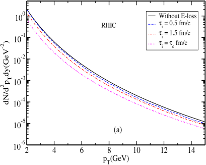
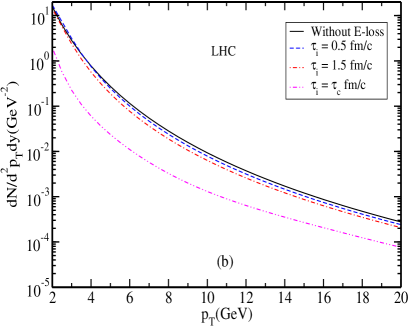
Figure 1: (Color online) $p_{T}$ distribution of parton at (a) RHIC energy (${T_{i}}=0.446$ GeV and ${\tau_{i}}=0.147$ fm/c) and at (b) LHC energy ($T_{i}=0.897$ GeV, $\tau_{i}=0.073$ fm/c).

However, in the above treatment, the infra-red cut-off is fixed by plasma effects, where only the medium part is considered, completely neglecting the vacuum contribution leading to ambiguity in the energy loss calculation. If the latter part is taken into account the strong coupling should be running. Thus for any consistent calculation one has to take into consideration this fact. In that case $\alpha_{s}=\alpha_{s}(k,T)$ ($k=\sqrt{|\omega^{2}-q^{2}|}$ in this case), and the above integrals must be evaluated numerically where the infra-red cut-off is fixed by Debye mass to be solved self-consistently:

$${m_{D}}(T)=4\pi\,\left(1+\frac{N_{F}}{6}\right)\,\alpha_{s}(m_{D}(T),T)T^{2}$$ (8)

We reiterate that the matrix elements in Eqs. (4) and (7) contains the strong coupling which we take as running, i. e. $\alpha_{s}=\alpha_{s}(\sqrt{|\omega^{2}-q^{2}|},T)$. We chose the following parameterization of $\alpha_{s}$ which respects the perturbative ultra-violet (UV) behavior and the 3D infra-red (IR) point prd75054031 :

$$\alpha_{s}(k,T)=\frac{u_{1}\frac{k}{T}}{1+exp(u_{2}\frac{k}{T}-u_{3})}$$ (9)

$$+ \frac{v_{1}}{(1+exp(v_{2}\frac{k}{T}-v_{3}))(ln(e+(\frac{k}{\lambda_{s}})^{a}+(\frac{k}{\lambda_{s}})^{b})},$$

with $k=\sqrt{|\omega^{2}-q^{2}|}$ in this case. The parameters $a$, $b$ and $\lambda_{s}$ are given by $a=9.07$, $b=5.90$ and $\lambda_{s}=0.263$ GeV. For the limiting behavior ($k<<T$) of the coupling we choose,

$$u_{1}={\alpha^{*}}_{3d}(1+exp(-u_{3}))$$ (10)

Here ${\alpha^{*}}_{3d}$ and ${\alpha^{*}}_{s}$ denote the values of the IR fixed point of $SU(3)$ Yang-Mills theory in $d=3$ and $d=4$ dimensions, respectively. The remaining four parameters ($u_{2}=5.47,u_{3}=6.01,v_{2}=10.13$ and $v_{3}=9.27$) fit the numerical results for pure Yang-Mills theory obtained from the RG equations in Ref. Braun_Gies .

So far we have discussed about the collisional energy loss which, although, dominates at lower energies, is not the only mechanism of energy loss. As the energy increases radiative energy loss starts to dominate and hence cannot be neglected. In case of jet-photon production, since the photon energy is almost equal to the jet energy, one has to include the radiative loss to account for the high $p_{T}$ photons. However, in order to see the effects of both the collisional and radiative energy losses, one must develop a formalism in which both the mechanisms can be taken into account in a consistent manner. The two mechanisms are not entirely independent, i.e., the collisional loss may influence the radiative loss. Thus both should be included to calculate transport coefficients. Since there is no rigorous way to implement this, the approximate way is to define effective drag (diffusion) in the following manner:

$$\eta = \eta_{\rm coll}+\eta_{\rm rad}$$ (11)

$$= \frac{1}{E}\left[\left(\frac{dE}{dx}\right)_{\rm coll}+\left(\frac{dE}{dx}\right)_{\rm rad}\right]$$

where $\left(\frac{dE}{dx}\right)_{\rm coll}$ can be calculated from Eq. (4) keeping in mind that $\eta p_{i}=A_{i}$. The collisional (differential) energy loss $(dE/dx)_{\rm coll}$ can be calculated from Eq. (4) using the method described in roy06 . For running $\alpha_{s}$ it is given by,

$$\left(\frac{dE}{dx}\right)_{\rm coll}=\frac{4}{3}\pi(1+\frac{N_{f}}{6})T^{2}{\int^{s}}_{{m_{D}}^{2}}d|t|\frac{{\alpha_{s}}^{2}(\sqrt{|t|},T)}{|t|^{2}}|t|$$

(12)

Where, $s=2ET$, $E$ is the energy of the incident quark. The radiative energy loss is given by,

$$\left(\frac{dE}{dx}\right)_{\rm rad}=\frac{C_{F}\alpha_{s}(E,T)}{N(E)}\frac{L\mu^{2}}{\lambda_{g}}\ln(\frac{E}{\mu}),$$ (13)

where $N(E)$ is an energy dependent factor and $N(E\rightarrow\infty)=4$ if kinematic bounds are neglected gyulassy00prl . It is important to point out here that $N(E)=7.3,10.1,24.4$ for $E=500,50,5$ GeV respectively and $N(E\rightarrow\infty)=4$ (see the Ref. gyulassy00prl ). $L$ is the distance traversed by the jets in the plasma. Similarly we can define the effective diffusion coefficients.

Having known the drag and diffusion, we solve the FP equation using Green’s function techniques: If $P(\vec{p},t|\vec{p_{0}},t_{i})$ is a solution to Eq. (3) with the initial condition

$$P(\vec{p},t=t_{i}|\vec{p_{0}},t_{i})=\delta^{(3)}(\vec{p}-\vec{p_{0}})$$ (14)

the full solution with an arbitrary initial condition can be obtained as moore05

$$f(t,\vec{p})=\int d^{3}{\vec{p}_{0}}P(\vec{p},t|\vec{p_{0}},t_{i})f_{0}(\vec{p}_{0})$$ (15)

where for the initial condition $f(t=0,\vec{p})=f_{0}(p_{0})$ and $P(\vec{p},t|\vec{p_{0}},t_{i})$ is the Green’s function of the partial differential Eq. (2).

We assume here that the plasma expands only longitudinally (Bjorken expansion scenario bj ). The reason is the following. The transverse expansion will have two effects on the parton energy loss: (i) The expanding geometry will increase the duration of propagation, (ii) the same expansion will cause the parton density to fall along its path. These two effects partially compensate each other and the energy loss is almost the same as in the case without transverse expansion plb526 . Since we are considering the central rapidity region $(|\eta|<0.35)$ the arguments given above is not applicable in the case of longitudinal expansion scenario.

The solution with an arbitrary initial momentum distribution can now be written as rapp ,

$$E\frac{dN}{d^{3}p}=\int\,d^{3}p_{0}\,P(\vec{p},t|\vec{p_{0}},t_{i})E_{0}\frac{dN}{d^{3}p_{0}}\,$$ (16)

We use the initial parton $p_{T}$ distributions (at the formation time $t_{i}$) taken from dks ; muller :

$$\frac{dN}{d^{2}p_{0T}dy_{0}}|_{y_{0}=0}=\frac{KN_{0}}{(1+\frac{p_{0T}}{\beta})^{\alpha}},$$ (17)

where $K$ is a phenomenological factor ($\sim 1.5-2$) which takes into account the higher order effects. The values of the parameters are listed in Table. 1.

	RHIC		LHC
	$q$	$\bar{q}$	$q$	$\bar{q}$
$N_{0}~{}[1/GeV^{2}]$	$5.0\times 10^{2}$	$1.3\times 10^{2}$	$1.4\times 10^{4}$	$1.4\times 10^{5}$
$\beta~{}[GeV]$	1.6	1.9	0.61	0.32
$\alpha$	7.9	8.9	5.3	5.2

Table 1: Parameters for initial parton $p_{T}$ distribution.

We note that the parametric form of Eq. (17) may not represent the true picture of the jet $p_{T}$ distribution. In recent years, more sophisticated calculations have been done using different parameterizations of the parton distribution functions. The $p_{T}$ distribution used here might differ substantially from these calculations and the results presented here is correct upto a factor that might come from using the more state of the art calculation.

II.3 Space time evolution

In order to obtain the space-time integrated rate we first note that the phase space distribution function for the incoming jet in the mid rapidity region is given by (see Ref. prc72 for details)

$$f_{jet}(\vec{r},\vec{p},t^{\prime})|_{y=0} = \frac{(2\pi)^{3}\mathcal{P}(|{\vec{w}}_{r}|)~{}t_{i}}{\nu_{q}\sqrt{{t_{i}}^{2}-{z_{0}}^{2}}}\frac{1}{p_{T}}$$ (18)

$$\times \frac{dN}{d^{2}{p_{T}}dy}(p_{T},t^{\prime})\delta(z_{0})$$

where $\frac{dN}{d^{2}{p_{T}}dy}(p_{T},t^{\prime})$ can be obtained from Eq. (16). $t_{i}$ is the jet formation time and $\nu_{q}$ is the spin-color degeneracy factor. $z_{0}$ is the jet formation position in the direction of QGP expansion and $\mathcal{P}(|{\vec{w}}_{r}|)$ is the initial jet production probability distribution at the initial radial position ${\vec{w}}_{r}$ in the plane $z_{0}=0$, where

$$|{\vec{w}}_{r}| = (\vec{r}-(t^{\prime}-t_{i})~{}\frac{\vec{p}}{\vec{|p|}})\cdot\hat{r}$$ (19)

$$= \sqrt{(r\cos{\phi}-t^{\prime})^{2}+r^{2}\sin^{2}{\phi}}\ \ {\rm for}\ t_{i}\sim 0$$

and $\phi$ is the angle in the plane $z_{0}=0$ between the direction of the photon and the position where this photon has been produced. We assume the plasma expands only longitudinally. Thus using $d^{4}x=rdrdt^{\prime}d\phi dz$ and the expression for $f_{jet}$ from Eq. 17 we obtain the transverse momentum distribution of photon as follows prc72 ; kapusta :

$$\frac{dN^{\gamma}}{d^{2}p_{T}dy} = \int d^{4}x~{}\frac{dN^{\gamma}}{d^{4}xd^{2}p_{T}dy}$$

$$= \frac{(2\pi)^{3}}{\nu_{q}}{\int_{t_{i}}}^{t_{c}}dt^{\prime}{\int_{0}}^{R}rdr\int d\phi\mathcal{P}(\vec{w_{r}})$$

$$\times \frac{{\mathcal{N}_{i}}}{16(2\pi)^{7}E_{\gamma}}\int d{\hat{s}}d{\hat{t}}|\mathcal{M}_{i}|^{2}\int{dE_{1}dE_{2}}$$

$$\times \frac{1}{p_{1T}}\frac{dN}{dp_{1T}^{2}dy}(p_{1T},t^{\prime})\frac{f_{2}(E_{2})(1\pm f_{3}(E_{3}))}{\sqrt{a{E_{2}}^{2}+2bE_{2}+c}}$$

$f_{jet}$ is the distribution function of the jet quark (see Eq. (18)) and rest of the distribution functions i.e $f_{2},f_{3}$ are Fermi-Dirac or Bose-Einstein distributions. $\phi$ dependence occurs only in $\mathcal{P}(\vec{w_{r}})$. So the $\phi$ integration can be done analytically as in Ref. prc72 . The temperature profile is taken from Ref. prc72 .

Besides the thermal photons from QGP and hadronic matter we also calculate photons from initial hard scattering from the reaction of the type $h_{A}\,h_{B}\,\rightarrow\,\gamma\,X$ using perturbative QCD. We include the transverse momentum broadening in the initial state partons wong ; owens . The cross-section for this process can then be written in terms of elementary parton-parton cross-section multiplied by the partonic flux which depends on the parton distribution functions (PDF) for which we take CTEQ parameterization cteq . A phenomenological factor $K$ is used to take into account the higher order effects. We also include photons from fragmentation process.

III Results

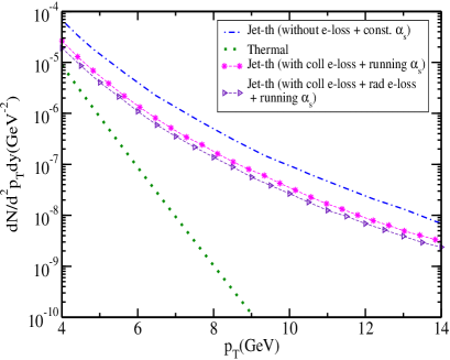
Figure 2: (Color online) $p_{T}$ distribution of photons at RHIC energy with ${T_{i}}=0.446$ GeV and ${\tau_{i}}=0.147$ fm/c. The violet (magenta) curve denotes the photon yield from jet-plasma interaction with collisional (collisional + radiative) energy loss. The blue curve corresponds to the case without any energy loss and the green curve represents the thermal contribution.

To obtain the quark momentum distribution we use Eqs. (3), (4), (7), (8) and (16). The transverse momentum distributions of quarks are shown in Fig. 1 for different times (proper) at RHIC and LHC energies respectively where the initial distributions are taken from Eq. (17). It is observed that the spectra are more reduced as the time increases. It is generally assumed that quarks fragment into hadrons around $\tau_{c}$ (the begining of the hadronic phase) where the quenching factor is the largest. At LHC energies (see Fig. 1b) this factor is more as the temperature in this case is large compared to RHIC energies. It is seen from Eq. (LABEL:last) the photon $p_{T}$ distribution is directly proportional to the quark $p_{T}$ spectra. Thus the photon yield will be affected as we shall see in the following.

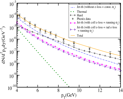
Figure 3: (Color online) $p_{T}$ distribution of photons at RHIC energy with ${T_{i}}=0.446$ GeV and ${\tau_{i}}=0.147$ fm/c. The magenta (blue) curve denotes the photon yield from jet-plasma interaction running (constant) $\alpha_{s}$. The black (green) curve corresponds to hard (thermal) photons. The orange represents the total photon yield compared with the Phenix measurements of photon data phenix .

In order to obtain the photon $p_{T}$ distribution we numerically integrate Eq. (LABEL:last) using Eq. (16). The results for jet-photons for RHIC energies are plotted in Fig. 2 where we have taken $T_{i}=446$ MeV and $t_{i}=0.147$ fm/c. As indicated earlier, the radiative energy loss starts dominating at higher energies of the jet, we include this in the calculation of photon $p_{T}$ distribution. We find that the yield is decreased with the inclusion of both the energy loss mechanisms as compared to the case when only collisional energy loss is considered. It is to be noted that when one considers collisional energy loss alone the yield with constant $\alpha_{s}$ is more compared to the situation when running $\alpha_{s}$ is taken into account. This is due to the fact that the energy loss in the later case is more prd75054031 . On the other hand, with the inclusion of the radiative loss the yield decreases further.

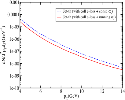
Figure 4: (Color online) $p_{T}$ distribution of jet-th photons at RHIC energy with ${T_{i}}=0.446$ GeV and ${\tau_{i}}=0.147$ fm/c. The red (blue) curve denotes the photon yield coming from jet-plasma interaction with collisional energy loss + running (constant) $\alpha_{s}$.

In order to compare our results with high $p_{T}$ photon data measured by the PHENIX collaboration phenix , we have to evaluate the contributions to the photons from other sources, that might contribute in this $p_{T}$ range. In Fig. 3 the results for jet-photons corresponding to the RHIC energies are shown, where we have taken $T_{i}=446$ MeV and $t_{i}=0.147$ fm/c. The individual contributions from hard and bremsstrahlung processes Owens are also shown for comparison. These are estimated using the formalism given in Ref. Owens . The total yield comprises of photons from jet-plasma interaction (with energy loss), hard and bremsstrahlung processes, thermal Compton and annihilation processes. We also show in a separate plot (in Fig. 4) photons from jet-plasma interaction corresponding to the cases with constant $\alpha_{s}$ and running $\alpha_{s}$ with collisional energy loss alone. It is observed that the spectra in the case of collisional energy loss with running coupling is depleted by a factor $1.7-2$ compared to the case where the strong coupling is constant. This is expected as the energy loss is more in the former case. The yield further reduces when both the mechanisms of energy loss are included. The total photon yield consisting of jet-photon, photons from initial hard collisions, jet-fragmentation and thermal photons is compared with the PHENIX photon data phenix . It is seen that the data is well reproduced in our model (see Fig. 3).

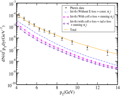
Figure 5: (Color online) $p_{T}$ distribution of photons at RHIC energies with $T_{i}=0.350$ GeV and $\tau_{i}=0.25$ fm/c. The orange line corresponds to total photon yield from all the sources as in Fig. 3 with both energy losses (collisional + radiative) included in the jet-photon contribution.

To cover the uncertainties in the initial conditions for a given beam energy, we consider another set of initial conditions at a lower temperature $T_{i}=0.350$ GeV and somewhat later initial time of $\tau_{i}=0.25$ fm/c. The yield for this set is shown in Fig. 5. We see that the data is reproduced reasonably well.

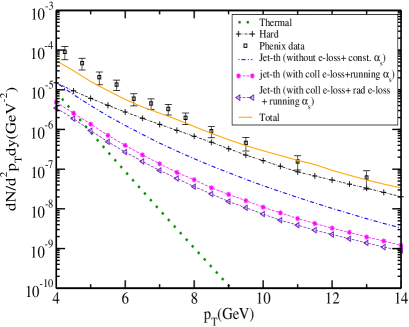
Figure 6: (Color online) $p_{T}$ distribution of photons at RHIC energy with ${T_{i}}=0.236$ GeV and ${\tau_{i}}=0.5$ fm/c. The magenta (blue) curve denotes the photon yield from jet-plasma interaction running (constant) $\alpha_{s}$. The black (green) curve corresponds to hard (thermal) photons. The orange represents the total yield compared with the Phenix measurements of photon data phenix .

In Fig. 6 we plot the $p_{T}$ distribution of photons for the RHIC energy ($T_{i}=0.236$ GeV and $\tau_{i}=0.5$ fm/c) for a lower value of $dN/dy=600$. It is clearly visible from Fig. 6 that we can not explain Phenix photon data satisfactorily in the $p_{T}$ range $4-8$ GeV. For the higher $p_{T}$ range Phenix photon data is well reproduced.

We also consider the high $p_{T}$ photon production at LHC energies. The contributions from various sources are shown in Figs. 7 where the jet-plasma contribution is calculated with running coupling constant ($\alpha_{s}$) (considering both the collisional and radiative energy losses). Since the initial temperature in this case is higher, the plasma lives for longer time. Thus the energy loss suffered by the parton is more. As a result, the difference between the cases with and without energy loss is slightly more than what is obtained at RHIC. It is observed that due to the inclusion of radiative energy loss along with collisional energy loss the jet photon yield is suppressed significantly. Also due to the inclusion of running coupling constant the jet photon yield is suppressed by a factor of $3-4$.

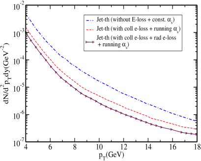
Figure 7: (Color online) Same as Fig.(3) at LHC energy ($T_{i}=0.897$ GeV and $\tau_{i}=0.073$ fm/c).

IV Summary

We have calculated the transverse momentum distribution of photons from jet plasma interaction with running coupling, i. e. with $\alpha_{s}=\alpha_{s}(k,T)$ where we have included both collisional and radiative energy losses. It is found that the assumption made in Ref. dks while calculating photons from jet-plasma interactions may not be good at LHC energies as we observe a difference is by a factor of $2-3$. Using running coupling we find that the depletion in the photon $p_{T}$ spectra is by a factor of $2-2.5$ more as compared to the case with constant coupling for RHIC energies. This is due to the fact that the energy loss (and hence drag and diffusion coefficients) is more by similar factor in the case of running coupling. Phenix photon data have been contrasted with the present calculation and the data seem to have been reproduced well in the low $p_{T}$ domain. The energy of the jet quark to produce photons in this range ($4<p_{T}<14$) is such that collisional energy loss plays important role here. It is shown that inclusion of radiative energy loss also describes the data reasonable well.

To check the sensitivity with the initial conditions, we consider two sets of initial conditions. In both the cases the data can be described quite well. This is due to the fact that both the initial conditions corresponds to the same $dN/dy=1150$.

As we validate our model through the description of Phenix photon data we also predict the high $p_{T}$ photon yield that might be expected in the future experiment at LHC. We notice that the inclusion of the radiative energy loss further reduces the yield at high $p_{T}$. It is observed that the contribution from jet-plasma interaction is slightly more reduced as compared to the RHIC case as the initial temperature is higher at LHC.

We do not consider transverse expansion as the energy loss of the partons remains just about the same as the case without transverse expansion. Finally, we conclude by noting that the role of running coupling constant should be explored in the context of other observables such as thermal photons, dileptons and so on.

References

- (1) J. Alam, S. Sarkar, P. Roy, T. Hatsuda, and B. Sinha, Ann. Phys. 286 159 (2000).
- (2) R. J. Fries, B. Muller, and D. K. Srivastava, Phys. Rev. Lett. 90, 132301 (2003).
- (3) P. Roy, J. Alam, S. Sarkar, B. Sinha, and S. Raha, Nucl. Phys. A624, 687 (1997).
- (4) J. Braun and H-J. Pirner, Phys. Rev. D75, 054031 (2007).
- (5) J. D. Bjorken, Fermilab-Pub-82/59-THY(1982) and Erratum (Unpublished); M. Gyulassy, P. Levai and I. Vitev, Nucl. Phys. B 571, 197 (2000); B. G. Zakharov, JETP Lett. 73, 49 (2001); M. Djordjevic and U. Heinz, Phys. Rev. Lett 101, 022302 (2008); R. Baier et al., J. High Ener. Phys. 0109, 033 (2001); S. Jeon and G. D. Moore, Phys. Rev. C71, 034901 (2005); A. K. Dutt-Mazumder, J. Alam, P. Roy, and B. Sinha, Phys. Rev. D 71, 094016 (2005); P. Roy, J. Alam, and A. K. Dutt-Mazumder, J. Phys. G. 35, 104047 (2008).
- (6) S. S. Adler et al., Phenix Collaboration, Phys. Rev. Lett.96 032301 (2006).
- (7) A. K. Dutt-Mazumder, J. Alam, P. Roy, B. Sinha, Phys. Rev. D71, 094016 (2005).
- (8) P. Roy, A. K. Dutt-Mazumder and J. Alam, Phys. Rev. C73, 044911 (2006).
- (9) A. Adil, M. Gyulassy, W. Horowitz and S. Wicks, Phy. Rev. C75 044906 (2007); M. Djordjevic, Phys. Rev. C74 064907 (2006); T. Renk, Phys. Rev. C76 064905 (2007).
- (10) S. Peigne, P. B. Gossiaux, and T. Gousset, J. High Energy Phys. 04, 011 (2006).
- (11) A. Ayala, J. Magnin, L. M. Montano, and E. Rojas, Phys. Rev. C77, 044904 (2008).
- (12) M. Gyulassy, I. Vitev, X. N. Wang, and B.W. Zhang, nucl-th/0302077.
- (13) P. B. Gossiaux and A. Aichelin, Phys. Rev. C78, 014904 (2008).
- (14) H. V. Hees and R. Rapp, Phys. Rev. C71 034907 (2005).
- (15) S. Wicks, W. Horowitz, M. Djordjevic, and M. Gyulassy, Nucl. Phys. A784, 426 (2007).
- (16) G -Y Qin, J. Ruppert, C. Gale, S. Jeon, G. Moore, and M. G. Mustafa, Phys. Rev. Lett 100, 072301 (2008).
- (17) M. H. Thoma, Phys. Lett. B273, 128 (1991).
- (18) K. Kajantie and P. V. Russkanen Phys. Lett. B121, 352 (1983).
- (19) R. D. Pisarski and E. Braaten, Nucl. Phys. B337, 569 (1990); ibid Nucl. Phys. B339, 310 (1990).
- (20) J. Alam, S. Raha and B. Sinha, Phys. Rev. Lett 73, 1895 (1994).
- (21) B. Svetitsky, Phys. Rev. D37, 2484 (1988).
- (22) G. D. Moore and D. Teaney, Phys. Rev. C71, 064904 (2005).
- (23) M. B. G. Ducati, V. P. Goncalves and L. F. Mackedanz, hep-ph/0506241.
- (24) J. Bjoraker and R. Venugopalan, Phys. Rev. C63, 024609 (2001).
- (25) G. Baym, Phys. Lett. B138 18 (1984).
- (26) M. H. Thoma and M. Gyulassy, Nucl. Phys. B351, 491(1991).
- (27) J. Braun and H. Gies, J. High energy Phys. 06 024 (2006).
- (28) M. Gyulassy, P. Levai and I. Vitev, Nucl. Phys. B571, 197 (2000).
- (29) J. D. Bjorken, Phys. Rev. D27 140 (1983).
- (30) M. Gyulassy, I. Vitev, X. N. Wang, and P. Huovinen, Phys. Lett. B526, 301 (2002).
- (31) B. Muller, Phys. Rev. C67 061901R (2003).
- (32) S. Turbide, C. Gale, S. Jeon and G. D. Moore, Phys. Rev. C72, 014906 (2005).
- (33) J. Kapusta, P. Lichard, and D. Seibert, Phys. Rev. D44 2774 (1991).
- (34) C. Y. Wong and H. Wang, Phys. Rev. C58, 376 (1998).
- (35) J. F. Owens, Rev. Mod. Phys. 59, 465 (1987).
- (36) J. Pumplin, D.R. Stump, J.Huston, H.L. Lai, P. Nadolsky, W.K. Tung, J. High Energy Phys. 012 0207 (2002).
- (37) S. S. Adler et al., Phys. Rev. Lett. 98 012002 (2007).
- (38) J. F. Owens, Reviews of Modern Physics, Vol-59, No. 2, 465 (1987).