Development of Richtmyer-Meshkov and Rayleigh-Taylor Instability in presence of magnetic field

Abstract

Fluid instabilities like Rayleigh-Taylor,Richtmyer-Meshkov and Kelvin-Helmholtz instability can occur in a wide range of physical phenomenon from astrophysical context to Inertial Confinement Fusion(ICF).Using Layzer’s potential flow model, we derive the analytical expressions of growth rate of bubble and spike for ideal magnetized fluid in R-T and R-M cases. In presence of transverse magnetic field the R-M and R-T instability are suppressed or enhanced depending on the direction of magnetic pressure and hydrodynamic pressure. Again the interface of two fluid may oscillate if both the fluids are conducting. However the magnetic field has no effect in linear case.
Keywords:Rayleigh-Taylor,Richtmyer-Meshkov instability,magnetic effect

1. Introduction

At the two fluid interface if heavier fluid is supported by lighter fluid, Rayleigh-Taylor instability (RTI) can occur. When a shock(storng/weak)is passed through the interface of two fluid the interface will be unstable and Richtmyer-Meshkov instability (RMI) can occur. The nonlinear structure resemble like a bubble(when the lighter fluid pushes across the unperturbed interface into the heavier fluid) and a spike (if the fluids are altered) arise due to this kind of fluid instability. RTI and RMI can occur from astrophysical situation to Inertial Confinement Fusion (ICF).

In ICF, high density fuel is compressed and accelerated towards the origin of the target sphere by multi KJ laser shock. During shock passage, the interface become unstable which inhibits the compression in the fusion process. Researchers are searching ways to stabilize these fluid instabilities. Using Layzer’s approximations several authors[1-3] derive the velocity of bubble and spike in linear and nonlinear domain. Magnetic fields can also be generated due to the ponderomotive force when the fluids are ionized [4,5]. The effect of magnetic field on Rayleigh - Taylor instability has been studied in details previously by Chandrasekhar [6]. The growth rate has been found to be lowered both for continuously accelerated (RTI) and impulsively accelerated (RMI) two fluid interface when $\vec{k}$ has a component parallel to the magnetic field [7,8].

Our paper is addressed to the problem of the temporal development of the nonlinear interfacial structure caused by RM and RT instability in presence of a magnetic field parallel to the surface of separation and perpendicular to the acceleration of the two fluids. The wave vector is assumed to lie in the same plane and perpendicular to the magnetic field.In this type of geometrical situation, no effect of the magnetic field is found in the linear approximation. However, in the nonlinear regime, the effect of magnetic field is predominant. It has been seen that the nonlinear growth rate may be enhanced or depressed according as the magnetic pressure contribution is either positive or negative. We have studied analytically and numerically the non linear behavior of the fluid interface in presence of magnetic field.

2. Basic equations and geometry of the problem

We have considered two infinite fluids of different constant density separated at $y=0$. The heavier fluid of density $\rho_{h}$ is along +ve y axis where as the lighter fluid of density $\rho_{l}$ lies along -ve y axis. Gravity also acts along-ve y direction. The magnetic field acts along $\hat{z}$ direction. So the Maxwell equation is easily valid i.e. $\vec{\nabla}.\vec{B}=0$.
After perturbation the finger like nonlinear surface is assumed to be parabolic

$$y(x,t)=\eta_{0}(t)+\eta_{2}(t)x^{2}$$ (1)

$$\mbox{where}\quad\quad\eta_{0}>0\quad\mbox{and}\quad\eta_{2}<0\quad\mbox{for bubble}\quad\qquad\qquad\eta_{0}<0\quad\mbox{and}\quad\eta_{2}>0\quad\mbox{spike}$$

Again we consider constant fluid density and hence equation of continuity gives $\vec{\nabla}.\vec{v}=0$, which satisfies the irrotational fluid motion. Since we are interested the motion the tip of the bubble, we can neglect the higher order term of $x^{i}(i\geq 3)$[9].

Now let us consider the potential function for heavier and lighter fluid, respectively,

$$\phi_{h}(x,y,t)=a_{1}(t)\cos{(kx)}e^{-k(y-\eta_{0}(t))};\quad y>0$$ (2)

$$\phi_{l}(x,y,t)=b_{0}(t)y+b_{1}(t)\cos{(kx)}e^{k(y-\eta_{0}(t))};\quad y<0$$ (3)

The fluid motion is governed by the ideal MHD equations

$$\rho\left[\frac{\partial\vec{v}}{\partial t}+(\vec{v}.\vec{\nabla})\vec{v}\right]=-\vec{\nabla}p-\rho\vec{g}+(\vec{J}\times\vec{B})$$ (4)

where $v=-\nabla\phi$ and $J=\frac{\nabla\times B}{\mu}$

$$\mbox{and magnetic induction equation}\quad\frac{\partial\vec{B}}{\partial t}=\vec{\nabla}\times[\vec{v}\times\vec{B}]$$ (5)

According to our magnetic field consideration

$$\frac{1}{\mu}(\vec{\nabla}\times\vec{B})\times\vec{B}=\frac{1}{\mu}(\vec{B}.\vec{\nabla})\vec{B}-\frac{1}{2\mu}\vec{\nabla}(\vec{B^{2}})$$ (6)

Using above relations and substituting in $\vec{v}$ in Eq. (4) followed by use of Eq. (6) leads to Bernoulli’s equation for the MHD fluid

$${\rho}\left[-\frac{\partial\phi}{\partial t}+\frac{1}{2}(\vec{\nabla}\phi)^{2}\right]=-{p}-\rho gy-\frac{1}{2\mu}{B}^{2}+{f(t)}$$ (7)

For RM instability the gravitation acceleration g should be replaced by$g=\Delta u\delta(t)$,where $\Delta u$ is the jump velocity at the interface and $\delta(t)$ is the delta function.

3. Kinematical and Dynamical boundary conditions at two fluid interface

The kinematical boundary conditions are

$$\frac{\partial\eta}{\partial t}+(v_{h})_{x}\frac{\partial\eta}{\partial x}=(v_{h})_{y}$$ (8)

$$(v_{h})_{x}\frac{\partial\eta}{\partial x}-(v_{l})_{x}\frac{\partial\eta}{\partial x}=(v_{h})_{y}-(v_{l})_{y}$$ (9)

The Bernoulli’s equations for both fluids are

$$\rho_{h}[-\frac{\partial\phi_{h}}{\partial t}+\frac{1}{2}(\vec{\nabla}\phi_{h})^{2}]-\rho_{l}[-\frac{\partial\phi_{l}}{\partial t}+\frac{1}{2}(\vec{\nabla}\phi_{l})^{2}]=-[g(\rho_{h}-\rho_{l})y+(p_{h}-p_{l})$$

$$+(\frac{{B^{2}}_{h}}{2\mu_{h}}-\frac{{B^{2}}_{l}}{2\mu_{l}})]+f_{h}(t)-f_{l}(t)$$ (10)

Further with the help of Eqs. (1) and (2) and the incompressibility condition $\vec{\nabla}.\vec{v_{h(l)}}=0$, Eq. (11) simplifies to

$$\frac{\partial[\vec{B}_{h(l)}(x,y,t)]}{\partial t}+(\vec{v}_{h(l)}.\vec{\nabla})\vec{B}_{h(l)}=0$$ (11)

The above Eqs.[8-11]give the temporal development bubble at the two fluid interface.

4. Equation for the structure and instability parameters

Substituting the $\frac{\partial\eta}{\partial x},\frac{\partial\eta}{\partial t}$ and expanding the velocity terms in powers of the transverse coordinate of x and keeping up to $x^{2}$,we obtain the following equations

$$\frac{d\xi_{1}}{d\ t}=\xi_{3}$$ (12)

$$\frac{d\xi_{2}}{d\ t}=-\frac{1}{2}(6\xi_{2}+1)\xi_{3}$$ (13)

$$b_{0}=-\frac{6\xi_{2}}{(3\xi_{2}-\frac{1}{2})}ka_{1}$$ (14)

$$b_{1}=\frac{(3\xi_{2}+\frac{1}{2})}{(3\xi_{2}-\frac{1}{2})}a_{1}$$ (15)

$$\xi_{1}=k\eta_{0};\qquad\xi_{2}=\eta_{2}/k;\qquad\xi_{3}=k^{2}a_{1}/\sqrt{kg}$$ (16)

Where $\xi_{1}$,$\xi_{2}$ and $\xi_{3}$ are nondimensionalized (with respect to the wave length) displacement,curvature and velocity of the tip of the bubble.

Now we are interested in magnetic field induction equations.We set the magnetic field induction equation to satisfy Maxwell’s relation as follows

$$B_{h}(x,y,t)=\beta_{h0}(t)+\beta_{h1}(t)\cos{(kx)}e^{-k(y-\eta_{0}(t))};\quad y>0$$ (17)

for heavier fluid and for lighter fluid

$$B_{l}(x,y,t)=\beta_{l0}(t)+\beta_{l1}(t)\cos{(kx)}e^{k(y-\eta_{0}(t))};$$ (18)

Using Eq. (11) and expanding the terms up to $x^{2}$for both magnetic field induction equations and we get

$$\dot{\beta}_{h0}(t)+(\dot{\beta}_{h1}(t)+\beta_{h1}(t)k\dot{\eta}_{0})\cos{(kx)}e^{-k(y-\eta_{0}(t))}-k^{2}a_{1}\beta_{h1}e^{-2k(y-\eta_{0}(t))}=0$$ (19)

for $x^{0}:$  ${\beta}_{h0}(t)+{\beta}_{h1}(t)=constant=B_{h0}\quad,say$ similarly for lighter fluid

$$\beta_{l0}(t)+\beta_{l1}(t)=constant=B_{l0}$$ (20)

For $x^{2}:$

$$\frac{\delta\dot{B}_{h}}{\delta B_{h}(t)}=\frac{(\xi_{2}-\frac{1}{2})}{(\xi_{2}+\frac{1}{2})}\xi_{3};\quad\delta B_{h}(t)=\frac{\beta_{h}(t)}{B_{h0}}$$ (21)

which gives

$$\delta{B}_{h}(t)=\delta{B}_{h}(t=0)\exp\left[{\int_{0}^{t}\xi_{3}\frac{(\xi_{2}-\frac{1}{2})}{(\xi_{2}+\frac{1}{2})}}d\tau\right]$$ (22)

Similarly for lighter fluid

$$\frac{\delta\dot{B}_{l}}{\delta B_{l}(t)}=\frac{(\xi_{2}+\frac{1}{2})}{(\xi_{2}-\frac{1}{2})}\frac{(\xi_{2}+\frac{1}{6})}{(\xi_{2}-\frac{1}{6})}\xi_{3};\quad\delta B_{l}(t)=\frac{\beta_{l}(t)}{B_{l0}}$$ (23)

Hence

$$\delta B_{l}(t)=\delta B_{l}(t=0)exp\left[{\int_{0}^{t}\xi_{3}\frac{(\xi_{2}+\frac{1}{2})}{(\xi_{2}-\frac{1}{2})}}\frac{(\xi_{2}+\frac{1}{6})}{(\xi_{2}-\frac{1}{6})}d\tau\right]$$ (24)

so that $\delta B_{h}(t)<(>0)$ if $\delta B_{h}(t=0)>(<0)$ and $\delta B_{l}(t)>0(<0)$ if $\delta B_{l}(t=0)>(<0)$.

The magnetic pressure difference at the two fluid interface will be

$$\frac{1}{2\mu_{h}}B^{2}_{h}(x,y,t)-\frac{1}{2\mu_{l}}B^{2}_{l}(x,y,t)=(\frac{B^{2}_{h0}}{2\mu_{h}}-\frac{B^{2}_{l0}}{2\mu_{l}})+k^{2}\left[\frac{{B^{2}}_{h0}}{\mu_{h}}\delta B_{h}(t)(\xi_{2}+\frac{1}{2})-\frac{{B^{2}}_{l0}}{\mu_{l}}\delta B_{l}(t)(\xi_{2}-\frac{1}{2})\right]x^{2}$$ (25)

Now the Bernoulli’s Eq.(10) becomes

$$\rho_{h}[-\frac{\partial\phi_{h}}{\partial t}+\frac{1}{2}(\vec{\nabla}\phi_{h})^{2}]-\rho_{l}[-\frac{\partial\phi_{l}}{\partial t}+\frac{1}{2}(\vec{\nabla}\phi_{l})^{2}]=-g(\rho_{h}-\rho_{l})y+k^{2}\frac{B^{2}_{h0}}{\mu_{h}}\delta B_{h}(t)(\xi_{2}+\frac{1}{2})x^{2}$$

$$+\frac{B^{2}_{l0}}{\mu_{l}}\delta B_{l}(t)(\xi_{2}-\frac{1}{2})x^{2}+f_{h}(t)-f_{l}(t)$$ (26)

Now we get the following nonlinear equation which describe temporal development of the tip of the bubble and the velocity of the bubble

$$\frac{d\xi_{1}}{d\tau}=\xi_{3}\hskip 750.0pt$$

$$\frac{d\xi_{2}}{d\tau}=-\frac{1}{2}(6\xi_{2}+1)\xi_{3}\hskip 690.0pt$$

$$\frac{\frac{d}{d\tau}{\delta B_{h}(t)}}{{\delta B_{h}(t)}}=\frac{(\xi_{2}-\frac{1}{2})}{(\xi_{2}+\frac{1}{2})}\xi_{3}\hskip 685.0pt$$

$$\frac{\frac{d}{d\tau}{\delta B_{l}(t)}}{{\delta B_{l}(t)}}=\frac{(\xi_{2}+\frac{1}{2})}{(\xi_{2}-\frac{1}{2})}\frac{(\xi_{2}+\frac{1}{6})}{(\xi_{2}-\frac{1}{6})}\xi_{3}\hskip 645.0pt$$

$$\frac{d\xi_{3}}{d\tau}=-\frac{N(\xi_{2},r)}{D(\xi_{2},r)}\frac{(\xi_{3}}{(6\xi_{2}-1)}+2(r-1)\frac{\xi_{2}(6\xi_{2}-1)}{D(\xi_{2},r)}\hskip 560.0pt$$

$$-\frac{(6\xi_{2}-1)}{D(\xi_{2},r)}[r\frac{kV^{2}_{h}}{g}\delta B_{h}(t)(2\xi_{2}+1)+\frac{kV^{2}_{l}}{g}\delta B_{l}(t)(2\xi_{2}-1)]\hskip 500.0pt$$

$$where,\tau=t\sqrt{kg};\quad r=\frac{\rho_{h}}{\rho_{l}};\quad D(\xi_{2},r)=12(1-r)\xi_{2}^{2}+4(1-r)\xi_{2}+(r+1);$$

$$N(\xi_{2},r)=36(1-r)\xi_{2}^{2}+12(4+r)\xi_{2}+(7-r);V_{h(l)}=\sqrt{B^{2}_{h0(l0)}/\rho_{h(l)}\mu_{h(l)}}$$ (28)

$V_{h(l)}$is the Alfven velocity in the heavier (lighter) fluid.

5. Asymptotic growth rate

To find out the asymptotic value of growth rate of bubble we set $d\xi_{2}/d\tau=0$ which gives $\xi_{2}=-1/6$ and at $\tau\rightarrow\infty$ integrating the last equation of the set of Eq.(27),

For RTI when lighter fluid is conducting:

$$[(\xi_{3})_{asymp}]_{bubble}=\sqrt{\frac{2Akg}{3(1+A)}}\sqrt{1-2(\frac{1-A}{A})\frac{kV^{2}_{l}}{g}[\delta B_{l}(\infty)]_{bubble}}$$ (29)

for spike

$$[(\xi_{3})_{asymp}]_{spike}=\sqrt{\frac{2Akg}{3(1-A)}}\sqrt{1-2(\frac{1+A}{A})\frac{kV^{2}_{l}}{g}[\delta B_{l}(\infty)]_{spike}}$$ (30)

and for RMI when the lighter fluid is conducting, the asymptotic growth rate is calculated omitting the second part of the last Eq. of the set of Eq.(27)and integrating,we get

$$[(\xi_{3})_{asymp}]_{bubble}=\sqrt{\frac{4V^{2}_{l}(1-A)}{3(\Delta u)^{2}(1+A)}\delta B_{l}(\infty)_{bubble}}cot\left[\left\{\frac{3(1+A)}{(1+A)}\sqrt{\frac{4V^{2}_{l}(1-A)}{3(\Delta u)^{2}(1+A)}\delta B_{l}(\infty)_{bubble}}\right\}\tau\right]$$ (31)

for spike

$$[(\xi_{3})_{asymp}]_{spike}=\sqrt{\frac{4V^{2}_{l}(1+A)}{3(\Delta u)^{2}(1-A)}\delta B_{l}(\infty)_{spike}}cot\left[\left\{\frac{3(1-A)}{(1-A)}\sqrt{\frac{4V^{2}_{l}(1+A)}{3(\Delta u)^{2}(1-A)}\delta B_{l}(\infty)_{spike}}\right\}\tau\right]$$ (32)

6. Results and discussions

We have solved the above set of equations using Runge-Kutta-Fehlberg method to describe the tip of the bubble and the velocity of the tip of the bubble for different cases.

Case 1

Assuming lighter fluid is conducting $B_{l0}\neq 0$ and the heavier one nonconducting, the hydrodynamic pressure driven force is suppressed by magnetic pressure.In case of weak shock the RMI also suppress.For density ratio $\rho_{h}/\rho_{l}=r=1.5,$ it has been seen that RT instability is suppressed (Fig.1).The RM instability is also suppressed in such situation (Fig.2).If the density ratio is increased, the Atwood number increases,consequently the growth rate increases. The growth rate may decrease if the density ratio is decreased.

Case 2

If the heavier fluid is conducting and lighter one nonconducting, the magnetic pressure acts along +ve y direction which increases the bubble growth for both case RT(Fig.3) and RM(Fig.4).

Case 3

If both the fluids are conducting the magnetic pressure difference and hydrodynamical pressure difference act in different direction and also in opposite phase at the interface.Hence the bubble will shows oscillatory behavior for both cases. For weak shock the oscillation frequency will be increased with the Alfven velocity(Fig.5).

Applications:

Super Nova explosion starts in a white dwarf as a laminar deflagration and RT instability begins to act.In white dwarf, magnetic field $\sim 10^{8}$G at the surface and RT instability arising during type Ia supernova explosion is associated with the strong magnetic field[10]. In the solar corona, magnetic field exist in a range of few Gauss to kilo Gauss. The lower limit of magnetic field is $\sim$ 10-20 Gauss, having temperature $2\times 10^{6}$ k[11]. Our model suggest that RT instability may show oscillatory stabilization if the magnetic field is greater than 34 gauss in solar corona.

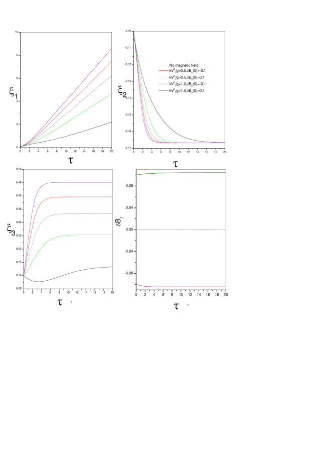
Figure 1: Variation of $\xi_{1}$, $\xi_{2}$,bubble growth rate $\xi_{3}(=\dot{\xi}_{1})$ and $\delta B_{l}$ with $\tau$ for $V^{2}_{h}=0$ for RTI . Initial values are $\xi_{1}=0.1,\xi_{2}=-0.1,\xi_{3}=0.1$ and $r=1.5$

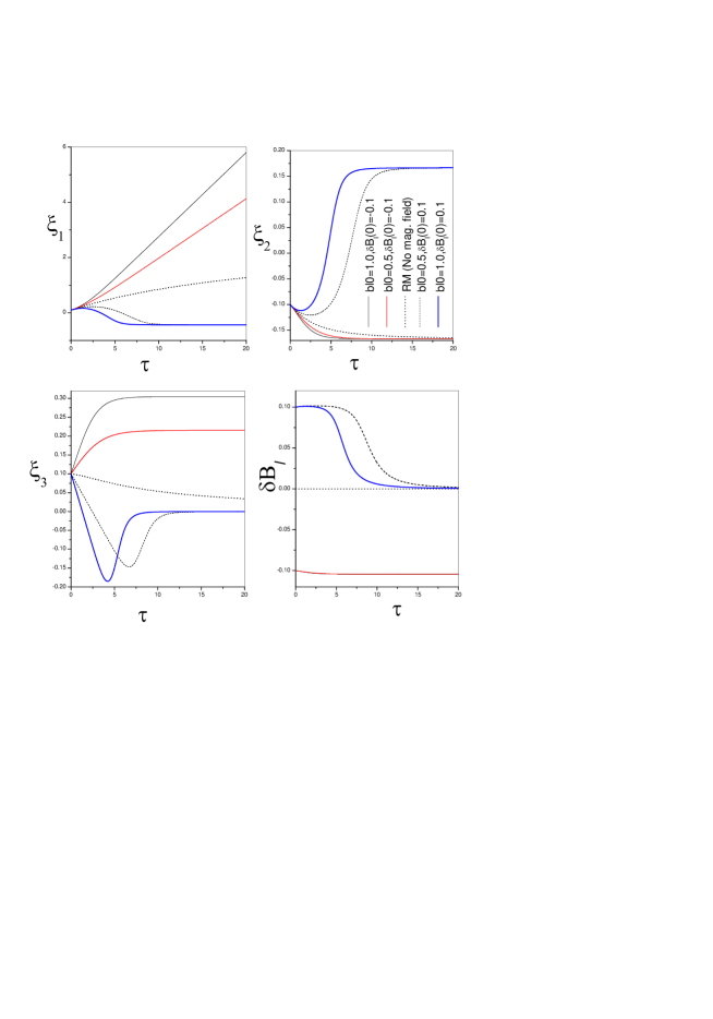
Figure 2: Variation of $\xi_{1}$, $\xi_{2}$,bubble growth rate $\xi_{3}(=\dot{\xi}_{1})$ and $\delta B_{l}$ with $\tau$ for $V^{2}_{h}=0$ for RMI . Initial values are as in fig1.

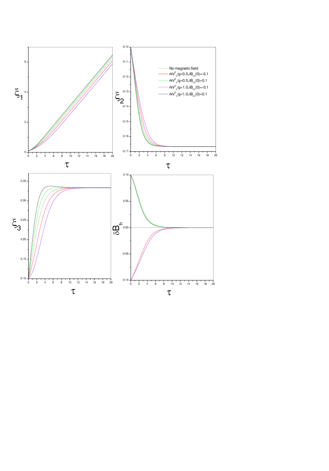
Figure 3: Variation of $\xi_{1}$, $\xi_{2}$, bubble growth rate $\xi_{3}(=\dot{\xi}_{1})$ and $\delta B_{l}$ with $\tau$ for $V^{2}_{l}=0$for RTI .Initial values are as in fig1.

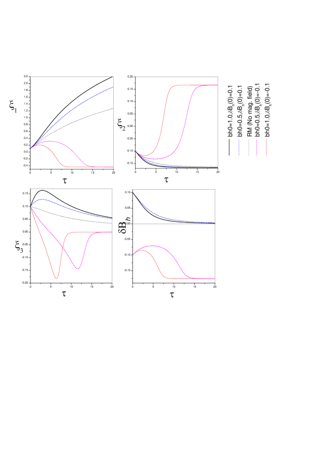
Figure 4: Variation of $\xi_{1}$, $\xi_{2}$, bubble growth rate $\xi_{3}(=\dot{\xi}_{1})$ and $\delta B_{h}$ with $\tau$ for $V^{2}_{l}=0$ for RMI.Initial values are as in fig1.

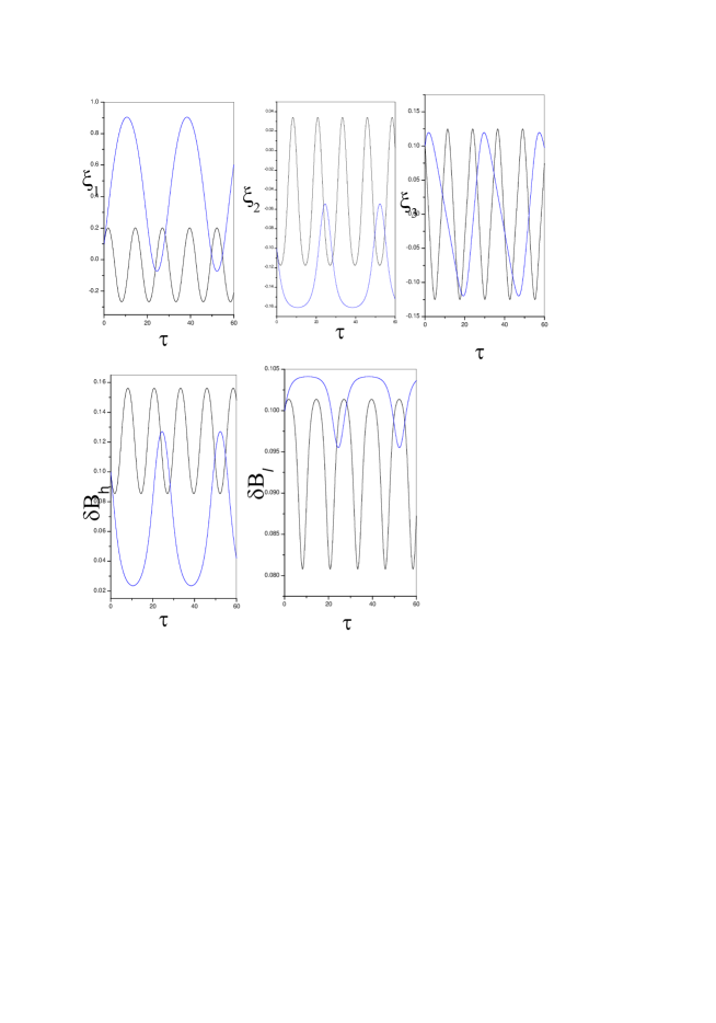
Figure 5: Variation of $\xi_{1}$, $\xi_{2}$, bubble growth rate $\xi_{3}(=\dot{\xi}_{1})$,$\delta B_{h}$ and $\delta B_{l}$with $\tau$. Initial values $\xi_{1}=0.1,\xi_{2}=-0.1,\xi_{3}=0.1,\delta B_{h}=\delta B_{l}=0.1,B_{h0}=B_{l0}=1.5$ and $r=1.5$ blue line for RTI and black line for RMI.

References

[1] J. Hecht, U. Alon and D. Shvarts, Phys. Fluids 6 (1994) 4019 .
[2] Qiang Zhang, Phys. Rev. Lett. 81 (1998) 3391 .
[3] V.N. Goncharov, Phy. Rev. Lett. 88 134502 (2002) .
[4] M.K.Srivastava,S.V.Lawande,Manoranjan Khan,Chandra Das and B.Chakraborty , Phys. Fluids B 4 (1992) 4086 .
[5] R.J.Mason and M.Tabak, Phys. Rev. Lett. 80 (1998) 524 .
[6] S. Chandrasekhar, Hydrodynamic and Hydromagnetic Stability, (Clarendon Press, Oxford,1968).
[7] V.Wheatley,D.I.Pullin, and R.Samtaney , Phys. Rev. Lett. 95 (2005) 125002 .