Fidelity Between Unitary Operators and the Generation of Gates Robust Against Off-Resonance Perturbations

Abstract

We perform a functional expansion of the fidelity between two unitary matrices in order to find the necessary conditions for the robust implementation of a target gate. Comparison of these conditions with those obtained from the Magnus expansion and Dyson series shows that they are equivalent in first order. By exploiting techniques from robust design optimization, we account for issues of experimental feasibility by introducing an additional criterion to the search for control pulses. This search is accomplished by exploring the competition between the multiple objectives in the implementation of the NOT gate by means of evolutionary multi-objective optimization.

To appear at J. Phys. A: Math. Theor.

1 Introduction

One of the challenges of coherent control of quantum systems is to achieve high fidelity in the presence of errors and/or noise that may be difficult or impossible to reduce by directly applying more precise controls. This situation is also exacerbated for systems with either complex underlying interactions or composed of heterogeneous ensembles. An example is the goal of achieving broadband inversion of spin ensembles [1, 2] and more generally broadband excitation of spin systems. Such needs have lead to the development of composite pulses [3, 4, 5, 6] which have been studied in the demanding field of quantum computing [7, 8, 9]. This technique was extended to include the use of shaped pulses [10, 11]. A more systematic approach is through the application of quantum optimal control [12, 13, 14, 15], with conceptual foundations lying in the control landscape topology for generating unitary transformations [16, 17]. The Magnus expansion is commonly used [20] to assess the robustness of implementing a unitary gate, in contrast to utilizing the Dyson series. The reason for this preference seems to arise from the fact that the Magnus expansion maintains unitarity while the truncated Dyson series does not. However, the fidelity between unitary matrices as an objective function is more naturally expressed in terms of the Dyson series. The next section validates the use of the Dyson series as an appropiate method for the assessment of robustness and shows how this relates with the Magnus expansion and the series expansion of the fidelity.

2 Formulating Conditions for Robustness

The optimal control of quantum gates for a system of $N$ discrete levels may be formulated in terms of the fidelity between two unitary operators as a scalar cost function

$$\mathcal{J}(U(T,0))\equiv\frac{1}{N}Re(Tr[W^{\dagger}U(T,0)]),$$ (1)

where $W$ is the target unitary operator [18], and the unitary evolution operator obeys the Schrödinger equation

$$i\frac{\partial}{\partial t}U=HU,$$ (2)

with $\hbar$ absorbed in the Hamiltonian and $T$ being the target time. A perturbation in the Hamiltonian $H\rightarrow H+\delta H$ implies a variation in $U$, which can be assimilated in an auxiliary operator $V$, defined such that

$$U\rightarrow U^{\prime}=UV.$$ (3)

The Schrödinger equation (2) implies

$$i\frac{d}{dt}V=\delta\hat{H}(t)V,$$ (4)

with $\delta\hat{H}(t)=U^{\dagger}(t,0)\delta H\,U(t,0)$. The solution of this equation can be expressed in terms of the Dyson series as

$$V(T,0)=\mathcal{T}e^{-i\int_{0}^{T}\delta\hat{H}(t)dt}=\mathbf{1}+\sum_{n=1}^{\infty}(-i)^{n}P_{n},$$ (5)

where $P_{n}$ are the time-ordered integrals

$$P_{n}=\int_{0}^{T}dt_{1}\int_{0}^{t_{1}}dt_{2}...\int_{0}^{t_{n-1}}dt_{n}\delta\hat{H}(t_{1})\delta\hat{H}(t_{2})...\delta\hat{H}(t_{n}),$$ (6)

with, for example $P_{1}=\int_{0}^{T}dt\,\delta\hat{H}(t)$.

Defining $\Delta U(T,0)=U^{\prime}(T,0)-U(T,0)$, the following expression can be obtained

$$\Delta U(T,0)=U(T,0)\sum_{n=1}^{\infty}(-i)^{n}P_{n}.$$ (7)

Equation (7) also can be written as a functional Taylor expansion,

$$\Delta U(T,0)=\sum_{n=1}^{\infty}\frac{1}{n!}\delta^{n}U(T,0),$$ (8)

which implies the following identity

$$\delta^{n}U(T,0)=n!\,U(T,0)(-i)^{n}P_{n}.$$ (9)

To proceed we define the action of the following brackets that specify the Hermitian and anti-Hermitian operators as well as the real trace

$$\langle X\rangle_{H} \equiv \frac{1}{2}(X+X^{\dagger})$$ (10)

$$\langle X\rangle_{A} \equiv \frac{1}{2}(X-X^{\dagger})$$ (11)

$$\langle X\rangle_{0} \equiv \frac{1}{N}Tr[\langle X\rangle_{H}]=\frac{1}{N}Re(Tr(X)),$$ (12)

such that we can verify the following identities

$$X=\langle X\rangle_{A}+\langle X\rangle_{H}$$ (13)

$$\langle\langle X\rangle_{A}\rangle_{H}=\langle\langle X\rangle_{H}\rangle_{A}=0$$ (14)

$$\langle\langle Y\rangle_{H}\langle X\rangle_{A}\rangle_{0}=0$$ (15)

$$\langle Y\langle X\rangle_{A}\rangle_{0}=\langle\langle Y\rangle_{A}\langle X\rangle_{A}\rangle_{0}$$ (16)

$$\langle Y\langle X\rangle_{H}\rangle_{0}=\langle\langle Y\rangle_{H}\langle X\rangle_{H}\rangle_{0}$$ (17)

With these definitions, the fidelity maybe written as

$$\mathcal{J}(U(T,0))=\langle W^{\dagger}U(T,0)\rangle_{0},$$ (18)

and the functional Taylor expansion of the fidelity takes the form

$$\Delta\mathcal{J}(U(T,0))=\sum_{n=1}^{\infty}\frac{1}{n!}\Big{\langle}W^{\dagger}\delta^{n}U(T,0)\Big{\rangle}_{0}$$ (19)

The first order term becomes

$$\Big{\langle}W^{\dagger}\delta U(T,0)\Big{\rangle}_{0}=\left\langle\langle W^{\dagger}U(T,0)\rangle_{A}(-i)P_{1}\right\rangle_{0},$$ (20)

which can be used to define the condition for the regular critical points of $\mathcal{J}(U)$ [19, 17] as

$$\langle W^{\dagger}U(T,0)\rangle_{A}=\frac{1}{2}(W^{\dagger}U(T,0)-U(T,0)^{\dagger}W)=0.$$ (21)

Thus, only the Hermitian part of $W^{\dagger}U(T,0)$ remains at the critical points

$$W^{\dagger}U(T,0)|_{critical}=\langle W^{\dagger}U(T,0)\rangle_{H}.$$ (22)

This implies that the expansion (19) evaluated at the regular critical points becomes

$$\Delta\mathcal{J}(U(T,0))|_{critical}=\sum_{n=2}^{\infty}{\Big{\langle}}\langle W^{\dagger}U(T,0)\rangle_{H}\left\langle(-i)^{n}P_{n}\right\rangle_{H}\Big{\rangle}_{0},$$ (23)

which can be used to identify the relevant factors $\left\langle(-i)^{n}P_{n}\right\rangle_{H}$ that depends on the control field. Elimination of the first order term characterizes a critical point and elimination of higher orders can be used as indicators of robustness. The robustness condition extracted from the second order term is

$$\left\langle(-i)^{2}P_{2}\right\rangle_{H}=0.$$ (24)

The Magnus expansion of a unitary operator [23], around the target $U(T,0)$ can be written as

$$W=U(T,0)\exp({\sum_{k=1}^{\infty}i\Omega_{k}}),$$ (25)

where $\Omega_{k}$ are Hermitian operators that can be written in terms of $P_{n}$ [24, 25] according to the identity

$$\sum_{k=1}^{\infty}i\Omega_{k}=\log(\mathbf{1}+\sum_{n=1}^{\infty}(-i)^{n}P_{n}).,$$ (26)

such that

$$i\Omega_{1} = -iP_{1}$$ (27)

$$i\Omega_{2} = -P_{2}+\frac{1}{2}P_{1}^{2}$$ (28)

$$i\Omega_{3} = iP_{3}+\frac{i}{3}P_{1}^{2}-\frac{i}{2}(P_{1}P_{2}+P_{2}P_{1})$$ (29)

$$i\Omega_{4} = P_{4}-\frac{1}{2}(P_{1}P_{3}+P_{3}P_{1})-\frac{1}{2}P_{2}^{2}+$$ (31)

$$\frac{1}{3}(P_{1}P_{1}P_{2}+P_{1}P_{2}P_{1}+P_{2}P_{1}P_{1})-\frac{1}{4}P_{1}^{4}$$

The criteria for robustness is based on sequential elimination of $\Omega_{k}$ [20, 21, 22], starting from the leading term

$$\Omega_{1}=0.$$ (32)

This condition implies $P_{1}=0$, which seems to be unrelated with the condition in (24). Applying condition (32) the leading terms of $i\Omega_{k}$ become

$$\Omega_{1} = 0$$ (33)

$$i\Omega_{2} = (-i)^{2}P_{2}$$ (34)

$$i\Omega_{3} = (-i^{3})P_{3}$$ (35)

$$i\Omega_{4} = (-i)^{4}P_{4}+\frac{1}{2}(-i)^{2}P_{2}^{2}.$$ (36)

Extracting the Hermitian part of each term

$$\langle i\Omega_{2}\rangle_{H} = \langle(-i)^{2}P_{2}\rangle_{H}$$ (37)

$$\langle i\Omega_{3}\rangle_{H} = \langle(-i)^{3}P_{3}\rangle_{H}$$ (38)

$$\langle i\Omega_{4}\rangle_{H} = \langle(-i)^{4}P_{4}\rangle_{H}+\frac{1}{2}\langle(-i)^{2}P_{2}^{2}\rangle_{H}$$ (39)

and recalling the anti-Hermiticity of each term of the the Magnus series $i\Omega_{n}$, one obtains

$$0 = \langle(-i)^{2}P_{2}\rangle_{H}$$ (40)

$$0 = \langle(-i)^{3}P_{3}\rangle_{H}$$ (41)

$$0 = \langle(-i)^{4}P_{4}\rangle_{H}+\frac{1}{2}\langle(-i)^{2}P_{2}^{2}\rangle_{H}.$$ (42)

indicating that $\Omega_{1}=0$ implies $\langle(-i)^{2}P_{2}\rangle_{H}=0$, showing the complete equivalence of conditions (32) and (24). Moreover, $\Omega_{1}=0$ also implies $\langle(-i)^{3}P_{3}\rangle_{H}=0$ and the relation $\langle(-i)^{4}P_{4}\rangle_{H}=-\frac{1}{2}\langle(-i)^{2}P_{2}^{2}\rangle_{H}$, which is useful for writing the two leading terms characterizing the robustness according with (23) as

$$P_{1} = 0$$ (43)

$$\langle P_{2}^{2}\rangle_{H} = 0.$$ (44)

However, the last condition can be further simplified considering $\left\langle P_{2}\right\rangle_{H}=0$ from (24) leading to the conditions on the Dyson series

$$P_{1} = 0$$ (45)

$$P_{2} = 0.$$ (46)

Moreover, these conditions are consistent if and only if

$$\Omega_{1} = 0$$ (47)

$$\Omega_{2} = 0.$$ (48)

Convergence of the Dyson series for N-level systems is assured if the field is bounded for a finite interaction time $T$ [26]. In contrast, convergence of the Magnus expansion demands more severe conditions [27]. The convergence is not relevant if the analysis is done in terms of the infinitesimal form of the perturbation Hamiltonian $\delta H$. However, in practice the perturbation Hamiltonian is finite, implying that the Magnus expansion may not necessarily converge. For this reason, any proposed robust implementation must be numerically verified for a finite range of small perturbations, as performed later in this paper, for a specific case.

3 NOT Gate

This section is concerned with the implementation of a robust NOT gate against off-resonant perturbations based on the lowest order condition $P_{1}=0$ for robustness. A general form for a single-qubit Hamiltonian with a resonant interaction is

$$H=\frac{1}{2}\omega_{0}\sigma_{3}+\boldsymbol{\Omega}(t)\sigma_{1}\cos(\omega_{0}t),$$ (49)

where $\boldsymbol{\Omega}(t)$ is the time-dependent modulated Rabi frequency. The corresponding time dependent Schrödinger equation is

$$H\psi=i\frac{\partial}{\partial t}\psi.$$ (50)

A transformation to the rotating frame will remove the diagonal term of the Hamiltonian. In the present case we consider a more general transformation with a time-dependent phase that can be controlled using a chirped pulse. The proposed transformation is

$$\psi=\mathcal{U}\Psi$$ (51)

with

$$\mathcal{U}=e^{-i(\omega_{0}t-\Phi(t))\sigma_{3}/2},$$ (52)

where $\Phi(t)$ is the accumulated off-resonant phase generated by chirping the pulse. The Schrödinger equation becomes

$$(\mathcal{U}^{\dagger}H\mathcal{U}-i\mathcal{U}^{\dagger}\frac{\partial}{\partial t}\mathcal{U})\Psi=i\frac{\partial}{\partial t}\Psi.$$ (53)

The first term is explicitly given as

$$\mathcal{U}^{\dagger}H\mathcal{U} = \frac{1}{2}\omega_{0}\sigma_{3}+\frac{\boldsymbol{\Omega}(t)}{2}\sigma_{1}(e^{i\omega_{0}t\sigma_{3}}+e^{-i\omega_{0}t\sigma_{3}})e^{-i(\omega_{0}t-\Phi(t))\sigma_{3}}$$ (54)

$$= \frac{1}{2}\omega_{0}\sigma_{3}+\frac{\boldsymbol{\Omega}(t)}{2}\sigma_{1}(e^{i\Phi(t)\sigma_{3}}+e^{(-2i\omega_{0}t+i\Phi(t))\sigma_{3}})$$ (55)

The last term is highly oscillatory if $\omega_{0}>>\Phi(t)$. This leads to a generalized rotating wave approximation as

$$\mathcal{U}^{\dagger}H\mathcal{U}\approx\frac{1}{2}\omega_{0}\sigma_{3}+\frac{\boldsymbol{\Omega}(t)}{2}\sigma_{1}e^{i\Phi(t)\sigma_{3}}.$$ (56)

Additional comments concerning the conditions specifying this approximation are found in A. The second term on the left side of (53) becomes

$$-i\mathcal{U}^{\dagger}\frac{\partial}{\partial t}\mathcal{U}=(-i)^{2}\frac{1}{2}\left(\omega_{0}-\frac{\partial\Phi(t)}{\partial t}\right)\sigma_{3}=(-\frac{1}{2}\omega_{0}+\frac{1}{2}\frac{\partial\Phi(t)}{\partial t})\sigma_{3}$$ (57)

and the final form of the Schrödinger equation in the rotating frame is

$$\left(\frac{1}{2}\frac{\partial\Phi(t)}{\partial t}\sigma_{3}+\frac{1}{2}\boldsymbol{\Omega}(t)\sigma_{1}e^{i\Phi(t)\sigma_{3}}\right)\Psi=i\frac{\partial}{\partial t}\Psi,$$ (58)

or, in a more expanded form

$$\left(\frac{1}{2}\frac{\partial\Phi(t)}{\partial t}\sigma_{3}+\frac{1}{2}\boldsymbol{\Omega}(t)(\cos\Phi\,\sigma_{1}+\sin\Phi\,\sigma_{2})\right)\Psi=i\frac{\partial}{\partial t}\Psi,$$ (59)

where both the off resonance phase $\Phi(t)$ and the Rabi frequency $\boldsymbol{\Omega}(t)$ are considered as the control functions. The term $\nu(t)=\frac{\partial\Phi(t)}{\partial t}$ is the shift of the resonant frequency as a function of time. It is important to note that the adiabatic condition was not required in the formulation above.

The simplest off-resonance perturbation is a constant, which can be modeled as

$$\delta H=\frac{\delta\epsilon_{0}}{2}\sigma_{3},$$ (60)

taking the following form in the interaction picture

$$\delta\hat{H}(t)=\frac{\delta\epsilon_{0}}{2}U^{\dagger}(t)\sigma_{3}U(t).$$ (61)

Consideration of this constant perturbation is restrictive, but a significant degree of robustness remains even for more general off-resonance perturbations including the important case of random perturbations as shown at the end of this section.

The NOT gate, up to a global phase, can be generated with the following unitary operator that may be implemented with a simple square pulse

$$NOT=e^{\frac{i}{2}\theta\sigma_{1}}|_{\theta=0\rightarrow\pi},$$ (62)

where the time of interaction occurs on the interval $t\in[0,T]$. Implementation of the robust gate can be achieved by introducing a composite unitary operator, which can be written as

$$U(\theta)=e^{\frac{i}{2}\theta\sigma_{1}}V(\theta),$$ (63)

with $V(\theta)=e^{\frac{i}{2}L(\theta)\sigma_{1}}e^{\frac{i}{2}R(\theta)\sigma_{3}}$, such that the following boundary conditions are imposed

$$L(0)=R(0)=L(\pi)=R(\pi)=0,$$ (64)

in order to ensure that $V(0)=V(\pi)=\mathbf{1}$. The associated Hamiltonian can be determined as

$$H=i\frac{\partial U}{\partial\theta}U^{\dagger},$$ (65)

where the energy is measured in units of $\frac{\pi\hbar}{T}$. This Hamiltonian may be explicitly evaluated as

$$H=-\frac{1}{2}(1+L^{\prime}(\theta))\sigma_{1}-\frac{1}{2}\sin[\theta+L(\theta)]R^{\prime}(\theta)\sigma_{2}-\frac{1}{2}\cos[\theta+L(\theta)]R^{\prime}(\theta)\sigma_{3},$$ (66)

which can be compared with (59) to identify

$$\boldsymbol{\Omega}(\theta) = \sqrt{(1+L^{\prime}(\theta))^{2}+\sin^{2}[\theta+L(\theta)]R^{\prime}(\theta)^{2}}$$ (67)

$$\nu(\theta) = -\cos(\theta+L(\theta)R^{\prime}(\theta)).$$ (68)

The boundary conditions (64) ensure that the target operator will be achieved, but it is necessary to impose additional conditions in order to assure that $\boldsymbol{\Omega}(\theta)$ is zero at the boundaries and therefore avoid sharp corners at the beginning and at the end of the pulse. The additional boundary conditions are

$$L^{\prime}(0)=L^{\prime}(\pi)=-1$$ (69)

Furthermore, we also require the modulation of the Rabi frequency $\boldsymbol{\Omega}(\theta)$ to be symmetric around $\pi/2$. The complete set of boundary conditions is satisfied by the following harmonic forms

$$L(\theta) = -\sum_{k=1}^{n}\frac{a_{k}}{2k}\sin(2k\theta)$$ (70)

$$R(\theta) = \sum_{k=1}^{n}b_{k}\sin(2k\theta),$$ (71)

for integer $n\geq 1$ and $\sum_{k=1}^{n}a_{k}=1$, where the coefficients are assumed to satisfy $|a_{k}|\leq 2\pi$ and $|b_{k}|\leq 2\pi$. Dropping the symmetry of $\boldsymbol{\Omega}(\theta)$ would result in $R(\theta)=\sum_{k=1}^{n}b_{k}\sin(k\theta)$.

The minimization of $P_{1}$ can be carried out through the numerical minimization of the following associated objective function for a finite number of harmonics $n$

$$J_{\delta\hat{H}}(a_{1},a_{2},...a_{n},b_{1},b_{2},...b_{n})=\left|\int_{0}^{\pi}U(\theta)^{\dagger}\sigma_{3}U(\theta)d\theta\right|,$$ (72)

with $a_{n}=1-\sum_{k=1}^{n-1}a_{k}$. The minimization of this cost function ensures a robust implementation of the target gate but there is the additional desire to implement the pulse with limited experimental resources. This problem can be addressed by introducing additional objective functions associated with the shape of $\boldsymbol{\Omega}(\theta)$ and $\nu(\theta)$. It is natural to consider a Gaussian form as model for $\boldsymbol{\Omega}(\theta)$ due to its smoothness and analytical properties

$$\hat{\Omega}(\theta)=A_{0}\exp{\left(-\frac{(\theta-\pi/2)^{2}}{2\sigma}\right)}.$$ (73)

The Gaussian function obeys the following differential equation

$$\hat{\Omega}^{\prime\prime}(\theta)=\hat{\Omega}^{\prime}(\theta)\left(\frac{\hat{\Omega}^{\prime}(\theta)}{\hat{\Omega}(\theta)}+\frac{1}{\theta-\frac{\pi}{2}}\right).$$ (74)

The following integral of the residual measures the degree of dissimilarity with respect to a Gaussian, thus, it can be used as a cost function for minimization

$$J_{\Omega}=\int_{0}^{\pi}d\theta\left|\boldsymbol{\Omega}^{\prime\prime}(\theta)-\boldsymbol{\Omega}^{\prime}(\theta)\left(\frac{\boldsymbol{\Omega}^{\prime}(\theta)}{\boldsymbol{\Omega}(\theta)}+\frac{1}{\theta-\frac{\pi}{2}}\right)\right|.$$ (75)

The same technique can be applied to the chirp frequency $\nu(\theta)$, but in this case the simplest chirp available in the laboratory is linear, which leads to the minimization of the following cost function

$$J_{\nu}=\int_{0}^{\pi}d\theta|\nu^{\prime\prime}(\theta)|.$$ (76)

In studies on robust design optimization, accounting for practical feasibility is typically carried out by introducing an additional criterion into the search for a control [28, 29]. We choose to follow this scheme, and therefore strive to explore the competition between $J_{\delta\hat{H}}$ and $J_{\Omega}$ by means of Pareto optimization, employing the MO-CMA-ES algorithm (for details, see B). A series of runs, considering five control parameters ($a_{1},~{}a_{2},~{}b_{1},~{}b_{2},~{}b_{3}$) and a population of 100 candidate solutions, produced the Pareto front shown in Figure 1. The front has an interesting shape, revealing a non-trivial conflict between $J_{\delta\hat{H}}$ and $J_{\Omega}$, yet allowing a reasonable trade-off, e.g., in the knee point shown in Figure 1 .

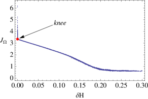
Figure 1: The attained approximate Pareto front describing the competition between $J_{\delta\hat{H}}$ and $J_{\Omega}$. The figure depicts the set of 300 non-dominated points, constructed by means of Pareto ranking of 10 fronts obtained in 10 individual runs. The enlarged dot is the knee point, chosen as the best compromise.

Setting a threshold of $J_{\delta\hat{H}}<0.0005$, the minimum value of $J_{\Omega}$ in the distribution is found to be $3.33$, which corresponds to the knee point. This point is characterized by the harmonics shown in Table 1. The corresponding plots of the Rabi modulation and chirp frequency are shown in Figures 2 and 3. The robustness of this implementation is evident in Figure 4, which shows the loss of fidelity as a function of the perturbation in comparison with an implementation with a square pulse (62). This figure also shows the response of the fidelity to a random Gaussian perturbation (instead of a constant perturbation) applied along the Pareto front. This figure implies that even though most random perturbations result in a fidelity lower than that obtained with a constant perturbation, there are some cases where the fidelity is actually higher.

n	$a_{n}$	$b_{n}$
1	0.896833	3.0578
2	0.302287	0.429276
3	-0.207685	0.0881475

Table 1: Set of harmonics that produce $J_{\delta\hat{H}}=0.00023$ and $J_{\Omega}=3.33$.

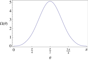
Figure 2: The modulation of the Rabi frequency $\boldsymbol{\Omega}(\theta)$ for the harmonics shown in Table 1.

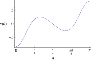
Figure 3: The chirp frequency $\nu(\theta)$ for the harmonics shown in Table 1.

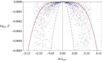
Figure 4: Fidelity plots of the square pulse (dashed lines) and optimized implementation of the NOT gate (solid curve), for the harmonics shown in Table 1. The fidelity is shown as a function of the perturbation amplitude normalized with respect to the maximum amplitude of $\boldsymbol{\Omega}(\theta)$. The dots show the response of the robust optimized implementation to a random Gaussian perturbation with mean $\epsilon$ and standard deviation $|\epsilon|/2$.

Upon deploying the MO-CMA-ES algorithm on a second bi-criteria minimization problem, where the chirp objective $J_{\nu}$ competes against the coherent average objective $J_{\delta\hat{H}}$, the redefined goal is observed to possess no conflict, which is not a priori evident. This is the case because the introduction of an additional objective usually leads to a conflict with the original objective(s). It is thus possible to obtain a robust implementation by practically ignoring the chirp. A solution of this kind is shown in Table 2. The respective plot of the Rabi frequency modulation is shown in Figure 5 and the response of the fidelity to perturbation is practically identical to that in Figure 4. Overall, this is a good illustration of scenarios where Pareto optimization may confirm or dispute the existence of competition between objectives where intuition may be misleading.

n	$a_{n}$	$b_{n}$
1	2.35701	$5.\times 10^{-7}$
2	-1.56989	$1.\times 10^{-7}$
3	0.21289	$1.\times 10^{-8}$

Table 2: Set of harmonics that produce $J_{\delta\hat{H}}=10^{-6}$ and $J_{\Omega}=0.00002$.

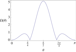
Figure 5: Modulation of the Rabi frequency $\boldsymbol{\Omega}(\theta)$ for the harmonics shown in Table 2.

In this section we proved that the robustness condition $P_{1}=0$ can be used to find a modulation of the Rabi frequency for a qubit system. This condition can in principle be applied to higher dimensions but in these cases the field cannot be directly extracted from the Schrödinger equation and more involved numerical techniques, such as D-MORPH [16], need to be applied.

4 Conclusions

We presented an analysis of the functional Taylor expansion of the fidelity between unitary operators with the aim of extracting conditions for the robust implementation of target gates. This expansion was written in terms of the Dyson expansion and compared with the Magnus expansion of unitary operators. The first order term of the fidelity expansion is zero when the target is achieved while higher orders are associated with the robustness of the implementation. The analysis of the Magnus expansion differs because the robustness is associated with all the higher order terms including the first one. We showed that the second order term of the fidelity expansion and the first order of the Magnus expansion are equivalent measures of the fidelity because eliminating either of them implies elimination of the other. This analysis was extended to the next leading order term showing additional connection between the fidelity and Magnus expansions.

Furthermore, we considered the implementation of the NOT gate as a case study, while taking into account an additional objective to obtain more desirable control pulse shapes. The competition between the objectives was successfully identified by means of an evolutionary multi-objective algorithm, allowing for a systematic exploration of the objectives and the nature of the conflicts. One case revealed an interesting Pareto front, with a promising trade-off area, while the competition in the other case was demonstrated to be non-existent despite initial expectations of conflict. This case study constitutes an example of a scenario where Pareto optimization is needed for balancing possibly conflicting gate control objectives, and at the same time assessing the validity of initial assumptions, often led by intuition.

Appendix A Generalized Rotating Wave Approximation

Section 3 makes use of a form of the rotating wave approximation. The justification of this approximation is best understood by analyzing the exact case and its limitations. The Schrödinger equation (53) without any approximation is

$$\frac{1}{2}\frac{\partial\Phi(t)}{\partial t}\sigma_{3}+\frac{1}{2}\boldsymbol{\Omega}(t)\cos(\omega_{0}t)(\cos(\Phi(t)-\omega_{0}t)\sigma_{1}+\sin(\Phi(t)-\omega_{0}t)\sigma_{2})\Psi=i\frac{\partial}{\partial t}\Psi,$$ (77)

which can be identified with (66) to obtain

$$-(1+L^{\prime}(\theta)) = \boldsymbol{\Omega}(\theta)\cos(\omega_{0}\theta)\cos(\Phi(\theta)-\omega_{0}\theta)$$ (78)

$$-\sin(\theta+L(\theta))R^{\prime}(\theta) = \boldsymbol{\Omega}(\theta)\cos(\omega_{0}\theta)\sin(\Phi(\theta)-\omega_{0}\theta)$$ (79)

$$-\cos(\theta+L(\theta))R^{\prime}(\theta) = \frac{\partial\Phi(\theta)}{\partial\theta},$$ (80)

such that the modulated Rabi frequency can be extracted as

$$\boldsymbol{\Omega}(\theta)=\frac{1}{|\cos(\omega_{0}\theta)|}\sqrt{(1+L^{\prime}(\theta))^{2}+\sin(\theta+L(\theta))^{2}R^{\prime}(\theta)^{2}}.$$ (81)

If the frequency of the free Hamiltonian $\omega_{0}$ is on the order of the Rabi frequency, there are possible singularities due to the division by $\cos(\omega_{0}\theta)$. These singularities can be lifted by proper selection of $L(\theta)$ and $R(\theta)$, but they are avoided altogether with a shorter pulse (larger Rabi frequency). Unfortunately, such a strong pulse may be difficult to implement experimentally and in extreme cases the conditions on the form of the dipole interaction may not be met. These situations are avoided in section 3 by taking a pulse which is weak enough to allow evolution under the free Hamiltonian to contain many cycles over the control interval.

Appendix B Pareto Optimization with Evolutionary Algorithms

Pareto optimization aims at simultaneously optimizing a number of conflicting objectives, and thereby revealing the Pareto optimal set or a region of interest in the trade-off surface between the objectives. In this appendix we summarize the principles of Pareto optimization, and especially provide some details on our employment of the method. Let a vector of objectives in $\mathbb{R}^{m}$,

$$\vec{f}\left(\vec{x}\right)=\left(f_{1}\left(\vec{x}\right),f_{2}\left(\vec{x}\right),\ldots,f_{m}\left(\vec{x}\right)\right)^{T},$$

be subject to minimization, and let a partial order be defined in the following manner. Given any $\vec{f}^{(1)}\in\mathbb{R}^{m}$ and $\vec{f}^{(2)}\in\mathbb{R}^{m}$, we state that $\vec{f}^{(1)}$ strictly Pareto dominates $\vec{f}^{(2)}$, which is denoted as

$$\vec{f}^{(1)}\prec\vec{f}^{(2)},$$

if and only if the following holds:

$$\forall i\in\{1,\dots m\}:f^{(1)}_{i}\leq f^{(2)}_{i}~{}\wedge~{}\exists i\in\{1,\dots,m\}:f^{(1)}_{i}<f^{(2)}_{i}$$ (82)

The crucial claim is that for any compact subset of $\mathbb{R}^{m}$, there exists a non-empty set of minimal elements with respect to the partial order $\preceq$ (see, e.g., [30]). Non-dominated points are then defined as the set of minimal elements with respect to the partial order $\preceq$. The aim of Pareto optimization is thus to obtain the non-dominated set and its pre-image in the control space, the so-called Pareto optimal set, also referred to as the efficient set. Finally, the Pareto front is defined as the set of all points in the objective space that correspond to the solutions in the Pareto-optimal set.

Evolutionary Algorithms (EAs) [31, 32], are powerful search methods, based on natural evolution, which have been successful in treating high-dimensional optimization problems. Here, we are especially interested in evolutionary multi-objective optimization algorithms (EMOA), which have undergone considerable development in the last two decades (see, e.g., [33, 34, 35]). Following the broad success of the Covariance Matrix Adaptation Evolution Strategy (CMA-ES) (see, e.g., [36]) in real-valued single-objective optimization, a multi-objective version has been released recently [37]. The Multi-Objective CMA-ES ( MO-CMA-ES) is the Pareto optimization approach used in our calculations.

In short, the CMA-ES is an evolution strategy variant that has been successful in treating correlations among decision (control) parameters by efficiently learning optimal mutation distributions. Explicitly, a set of $\mu$ search points comprise the evolving population of candidate solutions, which correspond to $\mu$ independently evolving single-parent CMA core strategies. The ultimate goal is thus to approximate the Pareto front of the given multi-objective optimization problem by means of these $\mu$ points. Given the $i^{th}$ search point in generation $(g)$ of the MO-CMA-ES, $\vec{x}^{(g)}_{i}$, an offspring is generated by means of a Gaussian variation:

$$\vec{x}^{(g+1)}_{i}\sim\mathcal{N}\left(\vec{x}^{(g)}_{i},\sigma^{(g)^{2}}_{i}\mathbf{C}^{(g)}_{i}\right)$$ (83)

The covariance matrices, $\left\{\mathbf{C}^{(g)}_{i}\right\}_{i=1}^{\mu}$, are initialized as unit matrices and are learned during the course of evolution, based on cumulative information of successful past mutations. The step-sizes, $\left\{\sigma^{(g)}_{i}\right\}_{i=1}^{\mu}$, are updated according to the so-called success rule based step-size control. The set of parents and offspring undergoes two evaluation phases, corresponding to two selection criteria: the first criterion is Pareto domination ranking, followed by the hypervolume contribution criterion. For more details we refer the reader to [37].

References

• [1] R.ย Tycko. Broadband Population Inversion. Physical Review Letters, 51(9):775โ€“777, 1983.
• [2] Jr-Shin Li and Navin Khaneja. Control of inhomogeneous quantum ensembles. Physical Review A (Atomic, Molecular, and Optical Physics), 73(3):030302, 2006.
• [3] M.H. Levitt. Composite pulses. Prog. Nucl. Magn. Reson. Spectrosc, 18:61โ€“122, 1986.
• [4] S.ย Wimperis. Broadband, narrowband and passband composite pulses for use in advanced NMR experiments. Journal of magnetic resonance. Series A(Print), 109(2):221โ€“231, 1994.
• [5] MJย Testolin, CDย Hill, CJย Wellard, and LCL Hollenberg. Robust controlled-NOT gate in the presence of large fabrication-induced variations of the exchange interaction strength. Physical Review A, 76(1):12302, 2007.
• [6] W.G. Alway and J.A. Jones. Arbitrary precision composite pulses for NMR quantum computing. eprint arXiv: 0709.0602, 2007.
• [7] H.K. Cummins, G.ย Llewellyn, and J.A. Jones. Tackling systematic errors in quantum logic gates with composite rotations. Physical Review A, 67(4):42308, 2003.
• [8] Kennethย R. Brown, Aramย W. Harrow, and Isaacย L. Chuang. Arbitrarily accurate composite pulse sequences. Phys. Rev. A, 70(5):052318, Nov 2004.
• [9] D.ย Mc Hugh and J.ย Twamley. Sixth-order robust gates for quantum control. Physical Review A, 71(1):12327, 2005.
• [10] Evanย M. Fortunato, Marcoย A. Pravia, Nicolas Boulant, Grum Teklemariam, Timothyย F. Havel, and Davidย G. Cory. Design of strongly modulating pulses to implement precise effective hamiltonians for quantum information processing. The Journal of Chemical Physics, 116(17):7599โ€“7606, 2002.
• [11] Matthias Steffen and Rogerย H. Koch. Shaped pulses for quantum computing. Physical Review A (Atomic, Molecular, and Optical Physics), 75(6):062326, 2007.
• [12] A.P. Peirce, M.A. Dahleh, and Herschel Rabitz. Optimal control of quantum-mechanical systems: Existence, numerical approximation, and applications. Physical Review A, 37(12):4950โ€“4964, 1988.
• [13] P.ย Brumer and M.ย Shapiro. Laser Control of Molecular Processes. Annual Reviews in Physical Chemistry, 43(1):257โ€“282, 1992.
• [14] B.ย Amstrup, J.ย D. Doll, R.ย A. Sauerbrey, G.ย Szabรณ, and A.ย Lorincz. Optimal control of quantum systems by chirped pulses. Phys. Rev. A, 48(5):3830โ€“3836, Nov 1993.
• [15] T.ย Schulte-Herbruggen, SJย Glaser, G.ย Dirr, and U.ย Helmke. Gradient Flows for Optimisation and Quantum Control: Foundations and Applications. focus, 13:14.
• [16] Raj Chakrabarti and Herschel Rabitz. Quantum control landscapes. International Reviews in Physical Chemistry, 26(4):671โ€“735, 2007.
• [17] Tak-San Ho, Jason Dominy, and Herschel Rabitz. Landscape of unitary transformations in controlled quantum dynamics. Physical Review A (Atomic, Molecular, and Optical Physics), 79(1):013422, 2009.
• [18] Herschel Rabitz, Michael Hsieh, and C.ย Rosenthal. Landscape for optimal control of quantum-mechanical unitary transformations. Physical Review A, 72(5):52337, 2005.
• [19] Michael Hsieh and Herschel Rabitz. Optimal control landscape for the generation of unitary transformations. Physical Review A (Atomic, Molecular, and Optical Physics), 77(4):042306, 2008.
• [20] Lorenza Viola, Emanuel Knill, and Seth Lloyd. Dynamical decoupling of open quantum systems. Phys. Rev. Lett., 82(12):2417โ€“2421, Mar 1999.
• [21] K.ย Khodjasteh and DAย Lidar. Fault-Tolerant Quantum Dynamical Decoupling. Physical Review Letters, 95(18):180501, 2005.
• [22] L.F. Santos and L.ย Viola. Advantages of randomization in coherent quantum dynamical control. New Journal of Physics, 10(083009):083009, 2008.
• [23] W.ย Magnus. On the exponential solution of differential equations for a linear operator. Communications on pure and applied mathematics, 7(4), 1954.
• [24] S.ย Blanes, F.ย Casas, J.A. Oteo, and J.ย Ros. The magnus expansion and some of its applications. Physics Reports, 470(5-6):151 โ€“ 238, 2009.
• [25] WRย Salzman. An alternative to the magnus expansion in time-dependent perturbation theory. The Journal of Chemical Physics, 82:822, 1985.
• [26] Abhra Mitra and Herschel Rabitz. Identifying mechanisms in the control of quantum dynamics through hamiltonian encoding. Phys. Rev. A, 67(3):033407, Mar 2003.
• [27] S.ย Blanes, F.ย Casas, JAย Oteo, and J.ย Ros. Magnus and Fer expansions for matrix differential equations: the convergence problem. J. Phys. A: Math. Gen, 31:259โ€“268, 1998.
• [28] Igorย N. Egorov, Gennadiyย V. Kretinin, and Igorย A. Leshchenko. How to Execute Robust Design Optimization. In 9th AIAA/ISSMO Symposium and Exhibit on Multidisciplinary Analysis and Optimization, September 2002.
• [29] Yaochu Jin and Bernhard Sendhoff. Trade-Off between Performance and Robustness: An Evolutionary Multiobjective Approach. In Proc.ย Evolutionary Multi-Criterion Optimization: Second Intโ€™l Conference (EMO 2003), volume 2632 of Lecture Notes in Computer Science, pages 237โ€“251, Berlin, 2003. Springer.
• [30] Matthias Ehrgott. Multicriteria Optimization. Springer, Berlin, second edition, 2005.
• [31] Thomas Bรคck. Evolutionary Algorithms in Theory and Practice. Oxford University Press, New York, NY, USA, 1996.
• [32] A.E. Eiben and J.E. Smith. Introduction to Evolutionary Computing. Springer, Berlin, 2007.
• [33] K.ย Deb. Multi-Objective Optimization Using Evolutionary Algorithms. Wiley, New York, 2001.
• [34] C.ย A.ย Coello Coello, G.ย B. Lamont, and D.ย A. VanVeldhuizen. Evolutionary Algorithms for Solving Multiobjective Problems. Springer, Berlin, 2007.
• [35] Joshua Knowles, David Corne, and Kalyanmoy Deb. Multiobjective Problem Solving from Nature: From Concepts to Applications. Natural Computing Series. Springer, Berlin, 2008.
• [36] Nikolaus Hansen and Stefan Kern. Evaluating the CMA Evolution Strategy on Multimodal Test Functions. In Parallel Problem Solving from Nature - PPSN V, volume 1498 of Lecture Notes in Computer Science, pages 282โ€“291, Amsterdam, 1998. Springer.
• [37] C.ย Igel, N.ย Hansen, and S.ย Roth. Covariance Matrix Adaptation for Multi-objective Optimization. Evolutionary Computation, 15(1):1โ€“28, 2007.