Star Clusters in M31: II. Old Cluster Metallicities and Ages from Hectospec Data

Abstract

We present new high signal$-$to$-$noise spectroscopic data on the M31 globular cluster (GC) system, obtained with the Hectospec multifiber spectrograph on the 6.5m MMT. More than 300 clusters have been observed at a resolution of 5Å and with a median S/N of 75 per Å, providing velocities with a median uncertainty of 6  km s^-1 . The primary focus of this paper is the determination of mean cluster metallicities, ages and reddenings. Metallicities were estimated using a calibration of Lick indices with [Fe/H] provided by Galactic GCs. These match well the metallicities of 24 M31 clusters determined from HST color$-$magnitude diagrams, the differences having an rms of 0.2 dex. The metallicity distribution is not generally bimodal, in strong distinction with the bimodal Galactic globular distribution. Rather, the M31 distribution shows a broad peak, centered at [Fe/H]=$-1$, possibly with minor peaks at [Fe/H]=$-1.4$, $-0.7$ and $-0.2$, suggesting that the cluster systems of M31 and the Milky Way had different formation histories. Ages for clusters with [Fe/H] $>-1$ were determined using the automatic stellar population analysis program EZ_Ages. We find no evidence for massive clusters in M31 with intermediate ages, those between 2 and 6 Gyr. Moreover, we find that the mean ages of the old GCs are remarkably constant over about a decade in metallicity ($-0.95\buildrel<\over{\sim}$ [Fe/H]$\buildrel<\over{\sim}0.0$).

1. Introduction

Star clusters in the Andromeda galaxy have been studied since Hubble (1932), and have long been known to comprise ages from young to old. It is the latter which are the topic of this paper. Initially, cataloging was all that was possible for clusters, work which indeed continues to this day with searches for distant clusters (Huxor et al., 2008). But spectroscopic studies as a means of measuring stellar populations and group kinematics also began early, starting with van den Bergh (1969), with substantial contributions by Huchra et al. (1982), Burstein et al. (1984), Tripicco (1989), Huchra et al. (1991), and Federici et al. (1993). Barmby et al. (2000) added much spectroscopy and photometry to the sample, and presented the largest study before the use of multiobject spectrographs on M31. At the time of the Barmby et al (2000) work, it was generally thought that the old M31 globular clusters (GCs) numbered several hundred, spanned a range of metallicity (as deduced from colors and absorption line strengths) equal to that of the galactic GCs, and likewise did not have a simple single Gaussian distribution of metallicities. The metal$-$poor clusters were thought to be roughly spherically distributed and to show a small amount of systemic rotation, while the most metal$-$rich clusters were thought to be confined to the disk of M31, and to show more systemic rotation, although the specifics of those and subsequent results will be further refined in this paper and other papers in this series.

Two large multifiber studies of M31 clusters have been presented in the last decade: Perrett et al. (2002) who used WYFFOS on the WHT, and Kim et al. (2007) who used Hydra on the WIYN telescope. The former paper produced more than 200 new velocities, and also found a bimodality of the old cluster metallicities, using spectral indices rather than colors. A subsequent kinematic analysis of those data by Morrison et al. (2004) suggested that the globulars could be explained using two kinematic components: a thin, cold rotating disk and a higher velocity dispersion component whose properties resemble M31’s bulge. The second study (where the kinematic results were presented in Lee et al., 2008) provided spectra for an additional 150 objects. However, in both studies, the kinematic analysis suffered from the inclusion of young disk clusters, which in particular led to statements that there were metal$-$poor clusters with thin disk kinematics (Morrison et al., 2004) or that the metal$-$poor clusters showed strong systemic rotation (Lee et al., 2008), in conflict with what Huchra et al. (1991) had reported, and what we will also conclude in a subsequent paper (A. Romanowsky et al., in preparation).

The important task of distinguishing M31’s young clusters from old was one of the topics in Caldwell et al. (2009, Paper I), made possible with new spectroscopy taken on the 6.5m MMT and using the Hectospec multi$-$fiber spectrograph (Fabricant et al., 2005). Ages and masses for more than 140 young clusters were determined by comparison with models, finding clusters with masses as great as $10^{4}M_{\sun}$, and a median cluster age of 0.25 Gyr. Table 1 of that paper also listed all the clusters, regardless of age, for which we added new information to the long$-$standing cataloging efforts by Galleti et al. (2007). That new information included revised coordinates, magnitudes, reddenings, and cluster classifications based on images and spectroscopy.

With the distinction between the young and old clusters now better clarified, we present here the first results of our high signal$-$to$-$noise (S/N) spectroscopic study of the old clusters in M31 (where we define old to be those with ages greater than 6 Gyr). This paper presents the velocities, ages and metallicities for the old clusters, and discusses the spatial, abundance and age properties of these clusters. The improved data allow us to revisit the topics addressed by previous authors. Where possible, we present comparisons with metal abundances derived from cluster color$-$magnitude diagrams (CMDs) using HST imaging, some of which is presented here. Subsequent papers will discuss kinematics and abundance ratios of these clusters.

We assume a distance of 770 kpc throughout (Freedman & Madore, 1990).

2. Spectroscopy

2.1. Sample

Subsequent to the publication of Paper I, more HST images of M31 clusters became available, which were inspected closely to further aid in the classification of objects in the cluster catalog. These images were particularly useful for objects in the bulge of M31, because the ground$-$based images (Massey et al., 2006) were often saturated in that high surface brightness area. There were no objects previously called clusters that are now thought to be stars, but several objects classified as stars based on spectra alone have been verified to be stars from these images. The Web site http://www.cfa.harvard.edu/oir/eg/m31clusters/
M31_Hectospec.html contains images for all old clusters, young clusters, stars and background galaxies in the catalog of Paper I, and may be profitably used to view individual cluster images as an adjunct to the spectroscopy of this paper. Spectra of the young clusters may also be found there; those of the old clusters will also appear there upon publication of this paper.

The observations we report on here are comprised of objects called “old” in Table 1 of Paper I; indeed those classifications were based on the information to be presented here.

2.2. Hectospec Observations

The data were all taken at the MMT with the Hectospec multifiber spectrograph (Fabricant et al., 2005) during the years 2004$-$2007. Twenty$-$five different but overlapping 1° diameter fields were observed, providing coverage except for an area due west of the center (Caldwell et al., 2009, Figure 2). Each field had targets of various kinds: clusters, HII regions and planetary nebulae, but the exact kind of cluster being observed, whether old or young, was often uncertain until the data were analyzed. Exposure times were typically 3600$-$4800s. Of the 367 clusters contained in our catalog (Caldwell et al., 2009) that we thought were old, we report on new spectra of 346, all but 26 of which we maintain are indeed old. We also report briefly on more than 30 clusters that appear to be younger than 2 Gyr upon further examination of their spectra, and which should have appeared in Table 2 of Paper I. A few cataloged old clusters within 1.°6 of M31’s center were missed in the spectroscopic observations either because they were outside of the area surveyed (the massive cluster G001 was missed for this reason), or initially had bad coordinates and were not re-observed after their coordinates had been corrected. There are as well several candidate clusters from Kim et al. (2007) that may be old clusters, judging from their ground-based images, but for which we have no spectra. These are concentrated in the disk of M31. Finally, aside of one case, we did not observe the outer clusters that have recently been discovered and cataloged by Huxor et al. (2008) and succeeding papers. The Hectospec fields covered a radius of about 1.6°= 21 kpc. Within that circle, there are 339 old clusters; we observed 316 of those, for a completeness of 93%.

Our spectra cover the wavelength range of 3700$-$9200 Å at 5Å resolution, with dispersion 1.2Å pixel^-1, and were reduced as described in Paper I. The fibers are 1.5˝ in diameter. Thus an important distinction needs to be made concerning the fraction of total cluster light these spectra represent, and the amount contained in typical spectra of galactic GCs. According to Barmby et al. (2007), the half-light radii of M31 GCs range from 0.5 to 1.0˝ . Thus, the Hectospec data sample the cluster light very well for most of the clusters. The Milky Way (MW) GC spectra by contrast sample mainly the cores of those clusters (Schiavon et al., 2005).

Sky subtraction was performed using several object-free spectra as near as possible to each target, except for targets in the bulge area, where the local background was high. In those cases, only sky spectra far from the bulge of M31 were used. A separate offset exposure for such fields, taken concurrently and about 5˝ offset from the targets, was reduced in a similar way (so that contemporaneous sky subtraction was performed for on- and off-target exposures), and then the off-target spectra were subtracted from the on-target. Tests done using spectra of the same bulge clusters reduced with and without the local background subtraction revealed errors of up to 100 km s^-1 and systematic errors of order 20 km s^-1 , if a local background was not used. The errors were in the sense that the observed velocities were pulled toward the velocity of the local background. Thus for this project local background measurements were crucial for obtaining accurate results, and this paper is the first to present precise velocities for a large number of clusters projected on the inner few kpc of M31.

The median S/N at 5200Å of the main set of spectra is 75 per Å, with some as high as 300 and others as low as 8 (Figure 1).

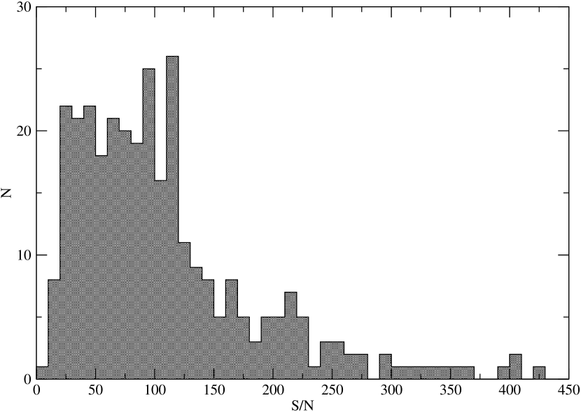
Figure 1.— Distribution of S/N at 5200 Å for 316 GC spectra.

The spectra were corrected to relative fluxes using standard star measurements taken at irregular intervals during the observation period. The spectrograph throughput was remarkably consistent over this period (Fabricant et al., 2008), thus we are confident in the corrections to fluxed spectra. The fluxing process was needed only for determining the reddening values.

A small number of clusters were observed with a higher ruling grating, which gave spectra with a resolution of 2.1Å over the range of $6000-8500$Å. These spectra are useful for velocities, but not for analyzing the stellar populations. Therefore, the ages of these clusters are still unknown.

2.3. Velocity Measurements

Subsequent to the Hectospec project, a HectoChelle project of many of these same targets was initiated (Strader & Caldwell, 2011), resulting in more precise velocities which allowed us to refine the Hectospec velocity zero$-$points. The HectoChelle spectra have a resolution of 30,000 and mean internal errors less than 1  km s^-1 (Szentgyorgyi et al., 1998) . In order to set the velocity zero$-$point for the Hectospec data, we first wavelength calibrated, and then set the velocities for the Hectospec spectra of 149 objects in common to be equal to the values found from the HectoChelle spectra. (There are 186 old clusters in total for which we have good HectoChelle spectra). These Hectospec spectra were then shifted and rebinned to zero$-$velocity, and combined into a single template. That template was then used as the cross$-$correlation template for the full set of Hectospec spectra, using the SAO xcsao software (Kurtz & Mink, 1998). By doing this, we minimized zero$-$point errors due to stellar template velocity errors and coarse spectral type mismatches that can occur when using a single star template on a composite spectrum. We did however include the entire range of metal abundances for the M31 GCs to make the template, thus there may still be some residual velocity errors due to template mismatching, for instance in a case where the cluster spectrum is very different from the mean cluster spectrum. The HectoChelle data (see below) proved to be a useful check on systematic errors.

The cross$-$correlation analysis for the Hectospec spectra used wavelengths from 4000-6800 Å, excluding wavelengths from 3700-4000 Å (the H&K region) even though the spectra cover that bluer region. If we incorporated that spectral region, we found a moderate dependence of velocity difference with velocity; as compared with the HectoChelle velocities. The trend was 20  km s^-1 over the range of 0 to $-$700  km s^-1 . This was probably the result of wavelength calibration errors for the bluest wavelengths. With the bluest spectral region excluded, the trend was reduced to 5  km s^-1 . The median offset in velocity became +2.9  km s^-1 (Spec$-$Chelle) and the rms became 5.7 km s^-1 . We did not remove this small residual offset from the velocities reported here.

Table Star Clusters in M31: II. Old Cluster Metallicities and Ages from Hectospec Data lists the objects believed to be old globular clusters from our sample, along with their coordinates, velocities and uncertainties. The other data presented in this table are discussed below. The velocities in this table come solely from the Hectospec data (with 3 exceptions where we had only HectoChelle data); the HectoChelle velocities will be reported in Strader & Caldwell (2011). Table 2 lists clusters thought to be old in Paper I, but which are now realized to be younger than 2 Gyr. Their velocities and uncertainties are also reported. The ages were determined as in Paper I, and again have uncertainties of about a factor of 2.

We can assess the quality of the Hectospec velocities in three ways: internally via repeated measurements, externally with the HectoChelle velocities, and externally with literature values. We have repeat observations for 213 GCs, some more than once for a total of 369 measurements. The median of the velocity differences is 1.2  km s^-1 , with an rms=8.8. This implies a median single measurement uncertainty of 6.2  km s^-1 . Figure 2 shows a histogram of these velocity repeat differences.

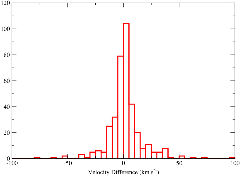
Figure 2.— Distribution of velocity differences derived from repeated measurements of 213 M31 GCs. The median of the velocity differences is 1.2  km s^-1, with an rms=8.8. This implies a median single measurement uncertainty of 6.2  km s^-1.

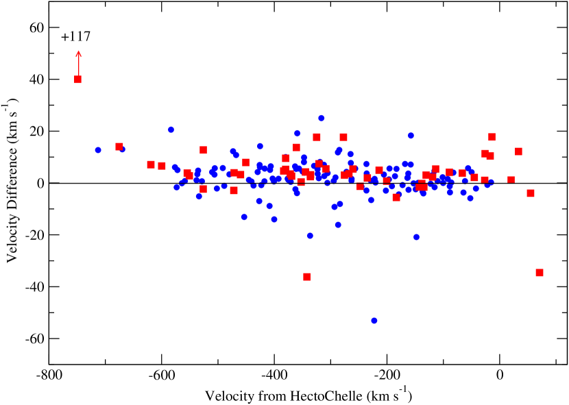
Figure 3.— Comparison with HectoChelle measurements. Velocity differences in the sense Hectospec - HectoChelle are plotted against the HectoChelle velocity. Squares indicate clusters in the bulge. The median offset in velocity is +2.9  km s^-1 (Spec$-$Chelle) and the rms is 5.7 km s^-1 . The worst case is that of B070-G133, which is just outside our defined bulge area, and thus its velocity may also be affected by bulge contamination.

Figure 3 shows the velocity differences of the 187 GCs that have HectoChelle velocities with cross correlation coefficients higher than 7, plotted against their velocities to allow the detection of velocity dependent errors. Four of these GCs have discrepant velocities in the Hectospec spectra: B070-G133 differs from the HectoChelle velocity by $-53$ km s^-1, B132 by $-35$ km s^-1, B262 by $-36$ km s^-1, and NB21 by $+117$ km s^-1. These errors probably resulted because all four are in the bulge. The first did not have an offset background exposure at all, and NB21 is the cluster closest to M31’s nucleus for which we have a spectrum, and thus it is the most affected by contamination from the surrounding light. The rms of the other 183 velocity differences is 5.7 km s^-1, whereas the median formal uncertainty in HectoChelle velocities is 0.5  km s^-1. Thus, the 5.7  km s^-1 is probably largely due to the Hectospec data, and therefore is close to the true median external uncertainty of objects in the Hectospec velocity catalog. The median Hectospec formal uncertainty from xcsao (the internal uncertainty) of those same objects is 9.8 km s^-1 , so the formal uncertainties listed in Table Star Clusters in M31: II. Old Cluster Metallicities and Ages from Hectospec Data are somewhat of an overestimate of the external uncertainties. For objects with listed uncertainties less than 20  km s^-1 , the external uncertainties can be estimated as $external=0.9+0.4*internal$. Figure 3 also shows the remaining zero$-$point offset of 3 km s^-1 and the remnant velocity$-$correlated velocity differences. The HectoChelle velocities will be presented in Strader & Caldwell (2011).

There are two large collections of M31 GC velocities with which we can compare our data, Barmby et al. (2000) and Perrett et al. (2002). There are not enough velocities in common with those reported by Kim et al. (2007) to construct a meaningful comparison. Figure LABEL:compare_vels shows a comparison of Hectospec velocities with those two sources. For the Perrett et al. (2002) comparison, there were two cases where the object called a cluster by that source was in fact a background galaxy; these we have excluded from the comparison. In the Barmby comparison, we have 186 objects in common, and the median velocity difference is $-$6  km s^-1 , with an rms of 90  km s^-1 . This is not too surprising given the heterogeneity of that catalog. For the Perrett comparison, there are 185 in common, with a median difference of $-$1 km s^-1, and an rms of 52 km s^-1, dropping to 30 if the remaining four worst, all of which are bulge clusters, are thrown out. Perrett quoted an overall uncertainty of 12 km s^-1, thus we find their uncertainties to be underestimates. Comparison of the Perrett velocities with the HectoChelle velocities allows us to derive a median uncertainty of 26  km s^-1 for their data set.

After putting them on a flux scale, the spectra were corrected to zero$-$velocity using our derived velocities, in preparation for index measurements and reddening determination.

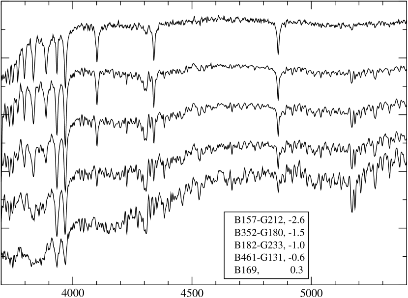
Figure 4.— Sample spectra from Hectospec. The [Fe/H] values are listed next to the objects’ names, and are those derived in this paper. The S/N ranges from 20 per Å (B169) to 100 (B182-G233) at 4000Å, and 50 to 200 at 5200Å. These spectra have been flux calibrated and Gaussian smoothed using a $\sigma=0.7$ Å. The full spectral coverage of 3650-9200Å has been truncated for display purposes.

Figure 4 shows a sample of the spectra, covering the full range of metallicities, which are described in the next section.

3. Cluster Metallicities via Milky Way GC Calibration

In this section we will discuss the measurement of the overall cluster metal abundances, characterized by [Fe/H], using absorption line indices from the M31 GC spectra. The indices can be converted to [Fe/H] using a calibration of the same indices found in the integrated spectra of Milky Way (MW) GCs, whose metallicities have previously been measured through abundance analysis of high resolution spectra of bona fide cluster member stars. Using such a calibration implicitly assumes that all the clusters, M31 and MW, are the same age. Thus we ignore not only the possibility that clusters in the two galaxies span a different range of ages, but also the observation that stars within many MW clusters may themselves have a range of ages (e.g., Piotto et al., 2007). The latter is very likely to be of negligible importance for the purposes of this study, as the age differences are found to be in most cases exceedingly small, or involve a small fraction of the total cluster’s stellar population. A larger difficulty is that the coarse Lick line indices we employ have complicated behaviors with [Fe/H]. For instance, the Fe, Mg b and Balmer indices all have a break in their relations at [Fe/H] values near $-1.5$. Also, the Balmer indices become insensitive at the high metallicity end, [Fe/H] $>-1$, which of course makes them useful when combined with an Fe index to determine ages and metallicities simultaneously, but useless to determine metallicities for metal$-$rich clusters. First, we will examine the distribution of the indices themselves.

3.1. Line Indices and Their Distribution

To measure the line indices, we used the lick_ew code, which is part of the EZ_Ages package (Graves & Schiavon, 2008). We smoothed the M31 spectra to the lower Lick/IDS resolution (see Worthey & Ottaviani (1997) for details) and measured the equivalent widths (EWs) adopting the passbands defined by Worthey et al. (1994) and Worthey & Ottaviani (1997). The instrumental EWs were converted to the Lick system (as redefined by Schiavon, 2007) using zero$-$points determined from measurements taken in spectra of six Lick standards also observed with Hectospec. These data, taken typically through one fiber only, were reduced following the same procedure as for the GC spectra and provided small zero point shifts used to convert the instrumental EWs into the Lick system. The details of the transformation to the standard Lick system will be covered in a subsequent paper (Schiavon et al. 2010, in preparation).

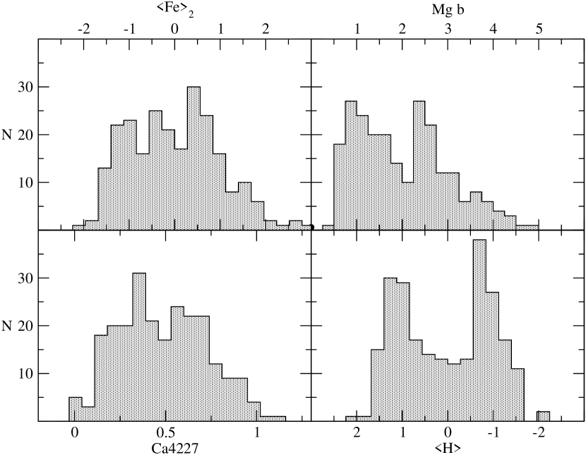
Figure 5.— Histogram of 4 different indices. The $\langle$Fe$\rangle_{2}$ and $\langle$H$\rangle$ indices are described in the text. Units are equivalent width in Å for Ca4227 and Mg b, standard deviations for the other two. Indices for 240 clusters with S/N $>$ 50 at 5200Å are shown here. Note that the X axis for $\langle$H$\rangle$ has been reversed so that metallicity increases to the right as in the other index plots.

Figure 5 shows the distribution of several selected indices: $\langle$Fe$\rangle_{2}$, Mg b, $\langle$H$\rangle$, and Ca4227. The $\langle$Fe$\rangle_{2}$ index is the average of 2 Lick Fe indices : Fe5270 and Fe5335, formed by converting the cluster values for each index to zero mean, unit variance values, and then averaging. $\langle$H$\rangle$ is the average of H$\delta_{\rm F}$, H$\gamma_{\rm F}$ and H$\beta$ indices (definitions contained in Worthey et al., 1994; Worthey & Ottaviani, 1997), formed in the same way. The index histograms are roughly bimodal, but complex. The conversions of these integrated light indices to [Fe/H] are not linear however, and thus the index distributions are not simple indicators of the underlying metallicity distribution, which we show below is neither unimodal nor bimodal.

3.2. [Fe/H] using Lick Fe indices

Early methods of ranking integrated light spectra of MW GCs by metallicities essentially used the similarity of the integrated spectra to those of single stars, and typed the cluster spectra as one would type a single star (Mayall, 1946; Morgan, 1956). Strong Balmer lines due to the presence of A-F stars indicated metal$-$poor clusters, while features due to G-K stars of course were found in metal$-$rich ones. Our method here for the M31 clusters derived from the methods of Da Costa & Mould (1988) and Brodie & Huchra (1990), who measured strong metallic lines in the spectra of MW GCs which had existing estimates for [Fe/H], and used the correlations of the line indices with [Fe/H] to then derive [Fe/H] values for extragalactic clusters. The difference in our method is that with our high S/N, we could make use of weaker lines that are more closely related to the actual Fe abundance in the stars of the clusters.

The disadvantage of our ignoring the stronger lines was that the uncertainties for the metal$-$poor clusters were larger than would have been the case had we considered such lines as the Balmer series or the Mg b lines. Galleti et al. (2009) recently used a heterogeneous set of spectra to estimate M31 GC metallicities, using a combination of weak and strong spectral features. Indeed, one can imagine other techniques that use more information in the spectra, perhaps in a $\chi^{2}$ matching method in comparison with a set of MW GC spectra, but given the incomplete set of MW GC spectra, that method is beyond the scope of this paper.

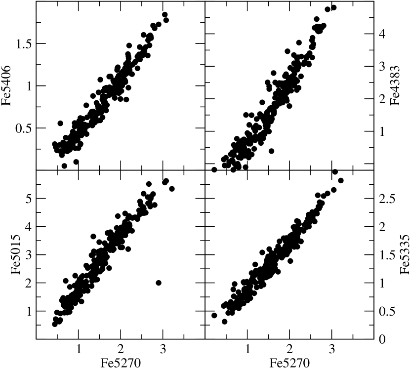
Figure 6.— Comparison of 5 Lick iron indices derived from the M31 GC spectra. Fe4383, Fe5015, Fe5335, and Fe5406 are plotted against Fe5270. The indices plotted here are from spectra with S/N $>$ 30 at 5200Å, typically the index uncertainties are less than 0.2Å. The discrepant point in the Fe5015 plot is B115-G177, which has strong [OIII]$\lambda 5007$ emission affecting the index measurement.

Figure 6 shows the mutual correlation of five Lick indices that were originally designed to measure Fe in stellar populations, and indeed they all correlate very well with each other. However, we calibrated the Lick indices with [Fe/H] using spectra of MW GCs, and one of those indices was not measurable using the available MW GC spectra. Also, including Fe4383 and Fe5406 did not improve the errors in the derived [Fe/H]. Thus we restricted ourselves to using an average, $\langle$Fe$\rangle$, of just the Fe5270 and Fe5335 indices to estimate [Fe/H].

The calibration was based on the library of MW GC spectra by (the “Tololo” sample, Schiavon et al., 2005). This library consists of flux-calibrated, intermediate-resolution, spectra of 41 Galactic GCs obtained with the Blanco 4 m telescope at CTIO. The spectral coverage is approximately 3350–6430 ${\rm\AA}$, and the spectral resolution $\sim$ 3.1 ${\rm\AA}$. Lick Fe indices were measured for the MW spectra in the same manner as for the M31 spectra.

The iron abundances spanned by the MW GCs in the Schiavon et al. (2005) study cover essentially the entire range of metallicities of the MW GC system ($-2.5<$ [Fe/H]$<0$) and are based on the metallicity scale of Carretta & Gratton (1997). Our relation between $\langle$Fe$\rangle$ and [Fe/H] for 31 MW clusters with Carretta & Gratton (1997) abundances is shown in Figure 7.

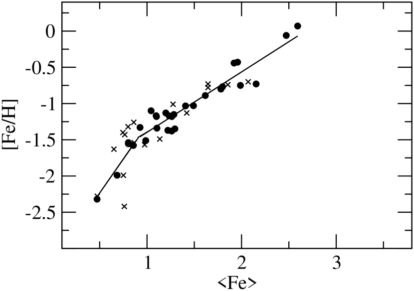
Figure 7.— Relation of the Lick $\langle$Fe$\rangle$ spectral index derived from the data of Schiavon et al. (2005) and [Fe/H] for Galactic Globulars (circles). This bi-linear relation was used to derive the [Fe/H] values for the M31 clusters. Crosses represent Lick indices of additional Galactic Globulars from Burstein et al. (1984). These were not used in the fit, but serve to confirm the validity of the fit.

A bi$-$linear fit was deemed to be best, and avoided the problems of wild extrapolated values that a quadratic or cubic fit would give. The transformation we derived is:

[Fe/H] = $-2.23+0.83*$ $\langle$Fe$\rangle$ ; for $\langle$Fe$\rangle$ $>0.9$;
[Fe/H] = $-3.18+1.88*$ $\langle$Fe$\rangle$ ; for $\langle$Fe$\rangle$ $\leq 0.9$.

Indices for different MW clusters reported in Burstein et al. (1984) are shown here as well to confirm the break in the relation (these were not used in deriving the bi$-$linear relation). Though we do not show them here, relations between [Fe/H] and Mg b and Balmer indices also showed a break. These breaks occurred at about [Fe/H]$=-1.2$ to $-1.5$, and like the one for $\langle$Fe$\rangle$, had the effect of broadening the low metallicity side of the index distributions when they were converted into metallicity distributions. Similar behavior was seen in the relation between line indices and MW GC [Fe/H] values shown in Galleti et al. (2009). If instead we used a single linear relation for any of these relations, the result was an overestimate of the metallicities of the most metal$-$poor clusters. Those with [Fe/H] $\simeq-2.5$ were then estimated to have [Fe/H] $\simeq-2.0$ while those with [Fe/H] $\simeq-1.8$ were then estimated to have [Fe/H] $\simeq-1.7$.

The MW GC bi$-$linear relation was then used to derive [Fe/H] values for the M31 clusters from these Lick indices, which are listed in Table Star Clusters in M31: II. Old Cluster Metallicities and Ages from Hectospec Data. We allow an extrapolation in [Fe/H] to $+0.3$, beyond the last MW GC data point at [Fe/H]$\sim-0.1$. For that reason, [Fe/H] values beyond that limit are obviously less reliable, though we do use a linear extrapolation. (Table Star Clusters in M31: II. Old Cluster Metallicities and Ages from Hectospec Data also includes the few clusters thought to be old based on their images that were observed only with the 600gpm grating centered at 7000Å. These were of course useful for velocities but not for the stellar population analysis. Thus, they have no [Fe/H] values listed. These include B056D and six clusters from the Kim et al. (2007) catalog.)

Now, the break in an index$-$[Fe/H] relation can transform the nature of the line index histogram from clearly bimodal to a more complex distribution, and this is what has apparently happened to our M31 data using our MW GC $\langle$Fe$\rangle$$-$[Fe/H] relation (see Figure 8, top panel), where the [Fe/H] histogram is not as obviously bimodal as is the $\langle$Fe$\rangle$ distribution. The GC color bimodality seen in most other external galaxies is taken to be caused by an intrinsic bimodality in the GC metallicity distribution (e.g., Brodie & Strader, 2006), but Yoon et al. (2006) examined the relation of color and metallicity, and found that relation also to be non$-$linear. Thus Yoon et al. doubted the universality of bimodal metallicity distributions in galaxies.

The uncertainties in the tabulated [Fe/H] values are derived from the statistical uncertainties in the $\langle$Fe$\rangle$ line indices used and from the formal uncertainties in the fit of [Fe/H] to the MW GC indices. Of course, there is an additional systematic uncertainty due to the choice of [Fe/H] values for the MW clusters used in the fit, the functional form of the fit that we chose, and the particular indices we chose to fit to [Fe/H]. To characterize one aspect of the systematic uncertainties, we show a comparison of the metallicity distributions of the entire M31 sample where the metallicities are derived from three different [Fe/H] calibrations, the adopted $\langle$Fe$\rangle$$-$[Fe/H] relation, and similar (bi$-$linear) relations involving Mg b and a Balmer index.

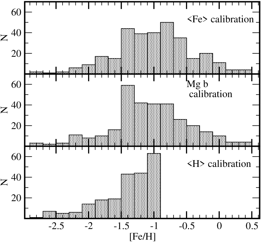
Figure 8.— Metallicity distribution of M31 GCs using three different calibration relations for transforming an index to [Fe/H]. Values in the top plot were derived using $\langle$Fe$\rangle$, those in the middle from Mg b, and those in the bottom plot from $\langle$H$\rangle$. Only the more metal-poor clusters are shown in the $\langle$H$\rangle$ panel, because the calibration is ill-defined for the more metal-rich clusters. This plot serves as an indication of the systematic errors in the [Fe/H] values contained in Table Star Clusters in M31: II. Old Cluster Metallicities and Ages from Hectospec Data.

These histograms are shown in Figure 8. The basic difference is a stronger peak at [Fe/H]=$-1.4$ from the Mg b relation, but otherwise the agreement is good. There is no systematic trend between the two determinations, and excluding five outliers, the rms between them is 0.18 dex for 316 clusters. The data for the [Fe/H] derived from $\langle$H$\rangle$ are cut off at [Fe/H]=$-1.0$ because the index has little sensitivity at higher metallicities. Still, it is clear that the strong bimodality shown in the $\langle$H$\rangle$ index distribution is not reflected in the derived metallicity distribution.

We do not consider the calibration of the Lick indices with [Fe/H] to be a solved question, though, and thus the resultant conclusions regarding the metallicity histogram (contained in Section 8 below) are preliminary. Clearly, more metal$-$poor MW GCs would address some of the shortcomings of the calibrations we have employed here, but verification of [Fe/H] values via individual stars for a representative sample of M31 GCs is also desirable.

4. Metallicities and Ages via Population Synthesis

Both ages and chemical composition estimates for the M31 GCs were obtained simultaneously from comparisons of the Lick indices with the SPS models from Schiavon (2007). The details of the models are contained in that paper, but in brief, polynomial functions describing the relations between various spectral indices and physical parameters of a stellar library were computed, and then combined with theoretical isochrones in order to produce predictions of integrated indices of single stellar populations. The isochrones employed were those from the Padova group for both the solar$-$scaled (Girardi et al., 2000) and $\alpha$$-$enhanced cases (Salasnich et al., 2000).

Figure 9 shows a comparison of data and models in two index$-$index diagrams. Both panels have the average $\langle$Fe$\rangle$ of the Lick Fe5270 and Fe5335 in the abscissa, plotted against Balmer line indices H$\beta$ and H$\delta_{F}$, in the top and bottom panels, respectively. Data points correspond to measurements of Lick indices in the spectra of 316 M31 GCs. Average error bars are displayed in the lower left corner on both panels. Because H$\beta$ and $\langle$Fe$\rangle$ are relatively insensitive to abundance ratio variations (for constant [Fe/H]), these indices provide reliable first guesses on the ages and iron abundances of the clusters under analysis.

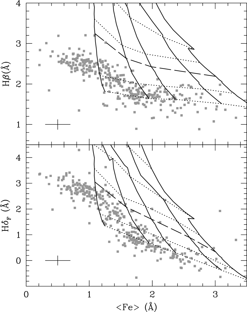
Figure 9.— Comparison between data for M31 GCs and the Schiavon (2007) models. Model same-[Fe/H] lines (solid), from left to right, are for [Fe/H] = $-$1.3, $-$0.7, $-$0.4, 0.0, and +0.2, whereas same-age lines (dashed), from bottom to top, are for 14, 8, 3.5, 2.5, 1.5, and 0.9 Gyr. Both panels show $\langle$Fe$\rangle$ (average of Lick indices Fe5270 and Fe5335) plotted against a Balmer line: H$\beta$ (top) and H$\delta_{F}$ (bottom). Average error bars are shown in the bottom left corner of each panel. Clusters with blue horizontal branches (mostly with [Fe/H] $\lesssim-1.0$) have artificially young ages. EZ_Ages does not deal with model extrapolations, and as a result, clusters outside the model grid are excluded from the analysis (see text for discussion).

Age and metallicity determination was achieved through application of the EZ_Ages code, developed by Graves & Schiavon (2008) for automatic stellar population analysis. EZ_Ages is an IDL implementation of a method developed by Schiavon (2007) to estimate the luminosity$-$weighted ages of stellar populations, as well as their luminosity$-$weighted abundances of iron, magnesium, carbon, nitrogen, and calcium, from Lick indices measured in their integrated spectra. The method has been successfully tested through application to Galactic GCs with known ages and chemical composition. Briefly, the method relies on a sequential grid inversion algorithm, which resolves for the parameters that fit best various index pairs, starting with age and the abundance that affects the most observables ([Fe/H]), then going down hierarchically to estimate abundances that impact fewer and fewer observables. Thus, adopting a first guess on the abundance pattern of the object stellar population, EZ_Ages finds the age and [Fe/H] combination that matches H$\beta$ and $\langle$Fe$\rangle$ best. Because these two indices are relatively insensitive to abundance$-$ratio variations, they provide a very good first guess on age and [Fe/H]. Assuming the latter values, EZ_Ages next finds the [Mg/Fe] value that provides a best match to magnesium$-$sensitive indices (Mg $b$ and/or Mg₂). Also adopting age and [Fe/H] inferred from the match to the H$\beta$$-$$\langle$Fe$\rangle$ pair, EZ_Ages finds the [C/Fe] abundance ratio that matches C${}_{2}4668$ best. Once that is known, it searches the [N/Fe] that matches CN indices best, then it finally finds the [Ca/Fe] abundance ratio that matches the Ca4227 index best. Note that the order in which those abundances are performed is important, given that CN indices are sensitive to the abundances of both carbon and nitrogen (as well as Fe), so that the abundance of the latter can only be determined once that of the former is known. Models with the new abundances are then used to redetermine age and [Fe/H] by returning to the H$\beta$$-$$\langle$Fe$\rangle$ pair, in order to account for their small sensitivity to abundance ratios. The process then is iterated until a final set of age and abundances is converged to. Convergence is typically achieved in no more than a couple of iterations. Readers interested in further details on both the models and EZ_Ages details on the models and age/abundance determination methods, are referred to Graves & Schiavon (2008) and Schiavon (2007). In this paper, we focus on the results for ages and [Fe/H], deferring the discussion of abundance ratios to a forthcoming paper (Schiavon et al. 2010, in preparation).

4.1. Caveats

Before discussing the ages and metallicities resulting from application of EZ_Ages to the data displayed in Figure 9, we highlight a few of the limitations of our method. First, EZ_Ages extrapolate from the models, and as a result, ages and abundances cannot be obtained for clusters falling off the model grids in Figure 9. Therefore, clusters with metallicities lower than [Fe/H]$\sim-1.3$, or higher than [Fe/H] $\sim+0.2$ are excluded from the analysis. Also excluded are clusters falling below the oldest models, for which EZ_Ages would find nonphysically old (i.e., older than the universe) solutions. Most of these clusters are in fact formally consistent with physically acceptable ages, given the index error bars. However, even after S/N considerations, a small minority of the clusters are still consistent with older$-$than$-$the$-$universe ages. This may possibly result from a combination of model zero$-$point uncertainties due to inadequate treatment of stellar luminosity function and abundance ratio effects (e.g., Schiavon et al., 2002) and Balmer$-$line infill from evolved giants and/or intra$-$cluster medium (Schiavon et al., 2005)—see Poole et al. (2010) for a discussion of this issue. Second, the treatment of horizontal branch stars in Padova isochrones, adopted in the Schiavon (2007) models, is such that there are blue horizontal branch stars in the metallicity range spanned by those models. As a result, metal$-$poor clusters with a blue HB tend to have stronger Balmer lines than predicted by models for the same age and metallicity, with the result that their ages are artificially younger according to the models. This can be seen on the top panel of Figure 9, where the ages of clusters with [Fe/H]$\buildrel<\over{\sim}-1.0$ are on average apparently $\sim$ 8 Gyr or younger. This is a well$-$known problem that has been discussed in detail in previous works (e.g., Freitas Pacheco & Barbuy, 1995; Lee et al., 2000), and which at present has no satisfactory solution, in view of the absence of a physically motivated theory capable of predicting the envelope mass (and consequently the effective temperature) of a star of given initial mass and chemical composition, when it reaches the core$-$He burning phase. Stellar population models relying on prescriptions based on free parameters have limited predictive power for ages. Our approach to this problem is that of singling out systems where the presence of blue HB stars may render spectroscopic age determinations unreliable. A method has been developed for that purpose by Schiavon et al. (2004), which relies on the differential effect of blue HB stars on higher and lower order Balmer lines (H$\delta$ and H$\beta$, respectively). Because blue HB stars are brighter in the blue they affect H$\delta_{F}$$-$based ages more strongly than those based on H$\beta$, which can be promptly seen from comparison of the top and bottom panels of Figure 9. Metal$-$poor GCs in the bottom panel appear to have “younger” ages than on the top panel, suggesting the presence of blue HB stars in these clusters. It is therefore not surprising that there is a significant difference between H$\beta$ and H$\delta_{F}$$-$based ages for clusters more metal$-$poor than [Fe/H]$\sim-0.95$ in the bottom panel of Figure 10. For these metal$-$poor clusters, ages from H$\beta$ and H$\delta_{F}$ differ by 2.7 $\pm$ 1.4 Gyr, and we deem their ages and abundances unreliable, excluding them from the present analysis.

4.2. EZ_Ages Results

Figure 10.— Top Panel: Ages and iron abundances resulting from application of EZ_Ages to the data shown in Figure 9. Bottom Panel: Difference between ages determined from $H\beta$ and $H\delta_{F}$, as a function of iron abundance. Ages for clusters more metal-poor than [Fe/H]$\sim-0.95$ can not be trusted due to the presence of blue horizontal branch stars, which are not considered in the Schiavon (2007) models, leading to artificially younger ages for metal-poor systems. The same effect is responsible to the systematic difference between the H$\beta$ and H$\delta_{F}$ ages for metal-poor systems in the bottom panel. Ages for clusters with [Fe/H] $\buildrel>\over{\sim}-0.95$ are reliable. See text for details.

Results from the application of EZ_Ages are shown in Figure 10. In the top panel, [Fe/H] is plotted against spectroscopic age for all the clusters falling within the model grids in the top panel of Figure 9. Following the above discussion, we do not consider clusters with [Fe/H]$\buildrel<\over{\sim}-0.95$. The higher metallicity group occupies a locus in the age$-$metallicity space characterized by a uniformly old population, with an age of 11.8 $\pm$ 1.9 Gyr, ranging in metallicity from [Fe/H]$\sim-0.95$ to solar. Because older clusters may have been left out of the analysis, and because of the model and data limitations discussed above, we make no claims on the absolute age of the oldest globular clusters in M31. On the other hand, EZ_Ages can provide very accurate relative ages (the internal age uncertainties are 2 Gyr), and with that in mind, we call attention to the fact that the mean ages of the old GCs in M31 seem to be remarkably constant over about a decade in metallicity ($-0.95\buildrel<\over{\sim}$ [Fe/H]$\buildrel<\over{\sim}0.0$). The apparent, small trend of age with metallicity could be artificially generated by a dependence of HB morphology with metallicity that is slightly different from that contained in the Tololo spectral sample, which is relatively devoid of clusters with blue HBs with $-0.95<$[Fe/H]$<-0.7$. This small trend will be examined in a future paper. One is of course also left wondering whether age remains nearly constant towards the lower metallicity regime, where age determination is unfortunately rendered unreliable due to the lingering gaps in our knowledge of stellar evolution in the post$-$He flash phase, as discussed above.

The ages found here are also recorded in Table Star Clusters in M31: II. Old Cluster Metallicities and Ages from Hectospec Data. However, the [Fe/H] values listed are those from Section 3.2 above, for reasons already discussed. If the indices for the cluster fell outside of the grids of Figure 9, or if the metallicity was lower than -0.95 as determined from the method of Section 3.2, the age was set to 14.

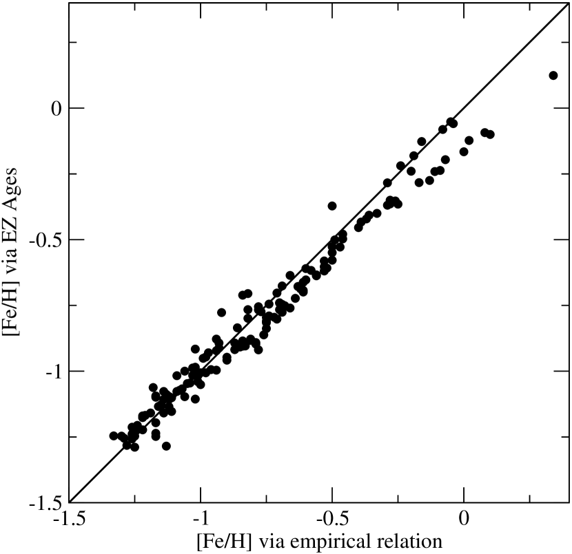
Figure 11.— [Fe/H] as derived by empirical fitting of galactic GC indices compared with [Fe/H] from EZ_Ages. The line represents equal values in the axes. For [Fe/H]$>-0.95$, the mean offset is small, between 0.05 and 0.08dex.

Figure 11 shows a comparison of [Fe/H] measured from Section 3.2 and the values using EZ_Ages. This indicates excellent agreement between the two methods for [Fe/H]$>-0.95$, with a small mean offset of 0.05$-$0.08dex. The detailed discussion of the M31 GC metallicity distribution will be taken up in Section 8. First, we compare the [Fe/H] values derived from the MW GC calibration with those from other sources.

5. Comparison of [Fe/H] with other measurements

5.1. [Fe/H] from other Integrated Light Studies

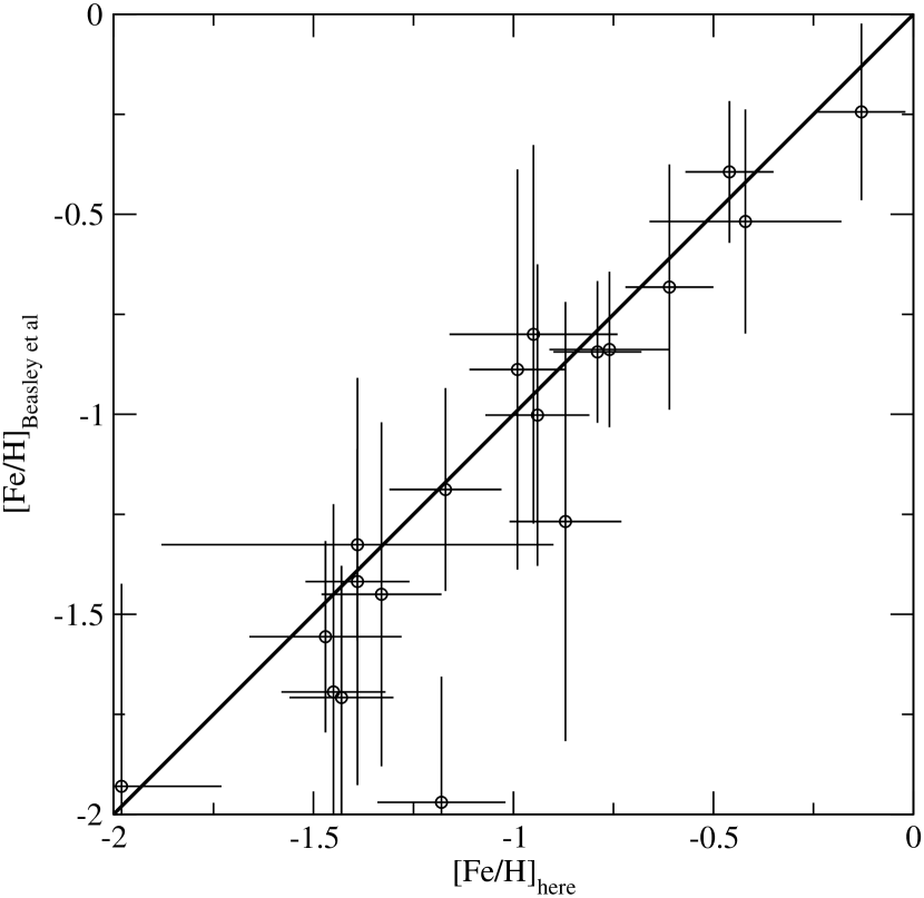
Figure 12.— Comparison of [Fe/H] derived from Hectospec spectra and inferred [Fe/H] values from Beasley et al. (2005), derived from spectra also taken with the MMT, but using the Blue Channel spectrograph. The stellar population models used for the Beasley results plotted here were those of Thomas et al. (2003). [Fe/H] values were calculated by using the published [Z/H] and [$\alpha$/Fe] values. The diagonal line represents equal values in the axes.

Beasley et al. (2005) derived [Z/H] values from MMT Blue Channel spectrograph spectra for 23 M31 objects. One of these is a star as noted below, otherwise we have 20 objects in common. Figure 12 shows a comparison of our [Fe/H] values derived from the MW GC Lick index calibration, and the Beasley et al. [Z/H] values converted to [Fe/H] using their published [Z/H] and [$\alpha$/Fe] values (and assuming that [Z/H]= [Fe/H] + 0.94[$\alpha$/Fe], from (Thomas et al., 2003). (Beasley et al. used two models to determine [Z/H] $-$ the differences between the two are small.) We find excellent agreement for the objects in common.

Colucci et al. (2009) measured [Fe/H], among other abundance ratios, for 5 M31 GCs using high resolution spectra and a method that matches observed equivalent widths of weak metallic lines with simple stellar population modelled equivalent widths. Four of their clusters are in common with our measurements (B045-G108, B381-G315, B386-G322, and B405-G351), and though the metallicity range is limited ($-0.86$ to $-1.22$), the mean offset is gratifyingly small, 0.08 dex, and the standard deviation of the differences is very small, 0.02 dex.

5.2. [Fe/H] from New Color$-$Magnitude Diagrams

We are fortunate that M31 is near enough to allow metallicity estimates to also be made using the mean colors of giant branch stars as resolved in HST imaging. Thus comparisons between [Fe/H] for clusters derived from spectra and CMDs can be performed. The HST/ACS images of the seven fields in the disk of M31 that were used to study the CMDs of several young clusters in Paper I also contain more than 10 old clusters. To add to the small but important literature of M31 CMDs, we have obtained point$-$spread function (PSF) photometry of five old clusters from that new data set (the other clusters are in extremely crowded fields). Data for four of these clusters were also analyzed by Perina et al. (2009). These HST data were processed as described in Paper I. In brief, we used the DAOPHOT package of Stetson (1987), modeling the spatially variable PSFs for each of the combined images separately, using only stars on those images. PSFs were constructed using $5-10$ bright stars which had no pixels above a level of 20,000 counts, the point at which an ostensible non$-$linearity sets in. Aperture corrections were also measured using these stars, to determine any photometric offset between the PSF photometry and the aperture magnitude within 0.5˝. Sirianni et al. (2005) have provided aperture corrections from that aperture size to infinity, in all Advanced Camera for Surveys (ACS) filters. The photometry was then placed on the standard Johnson/Kron-Cousins VI system using the aperture corrections and synthetic transformations provided in Sirianni et al. (2005). To lessen the severe problems with crowding in these clusters, only stars that fall in an annulus with radii of 15 and 50 pixels (0.75 and 2.5˝ ) from the center are shown in the color$-$magnitude diagrams (Figure 13).

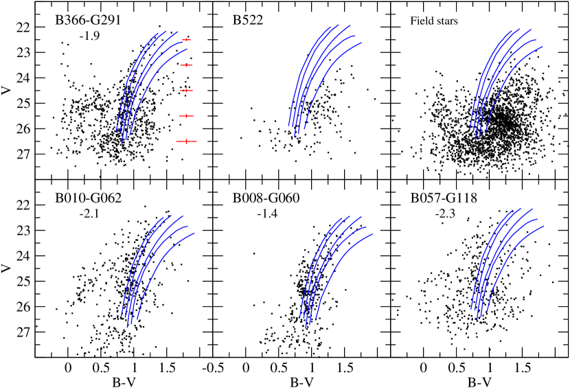
Figure 13.— CMDs of 5 old clusters and the field for B057-G118. Also shown are fiducial giant branches for 5 galactic globulars with a range of abundances : NGC4590 ([Fe/H]$=-2.3$), NGC 6809 ($-1.9$), NGC6752 ($-1.6$), NGC362 ($-1.3$) and 47 Tuc ($-0.8$) (G.S. Da Costa, priv.comm., metallicities from Carretta et al., 2009). Reddenings for the clusters listed in Table Star Clusters in M31: II. Old Cluster Metallicities and Ages from Hectospec Data were used to shift the fiducial curves. A distance modulus of 24.43 was assumed. Abundances of the M31 clusters as derived from these CMDs are shown, and are listed in Table 3 along with those derived from the spectra. Median photometric error bars are shown in the figure for B366-G291, at a range of magnitudes. The field stars were collected over an area 25 times larger than that for the clusters.

Figure 13 shows the CMDs of the five clusters, along with fiducial giant branches of galactic GCs, shifted assuming a distance modulus of 24.43 and the clusters’ reddenings derived below and listed in Table Star Clusters in M31: II. Old Cluster Metallicities and Ages from Hectospec Data. [Fe/H] values for the clusters were then visually estimated by the position of the observed giant branch compared to the fiducial branches, and the values are listed in Table 3. The uncertainties in the derived [Fe/H] values are 0.2 dex. A CMD comprised of field stars in an area 25 times larger than the cluster areas is also shown. B522 was too poor in giant stars for an estimate to be made. The giant branch of B057-G118 is bluer than our most metal$-$poor fiducial cluster, but we have left the derived metallicity at the minimum of $-2.3$.

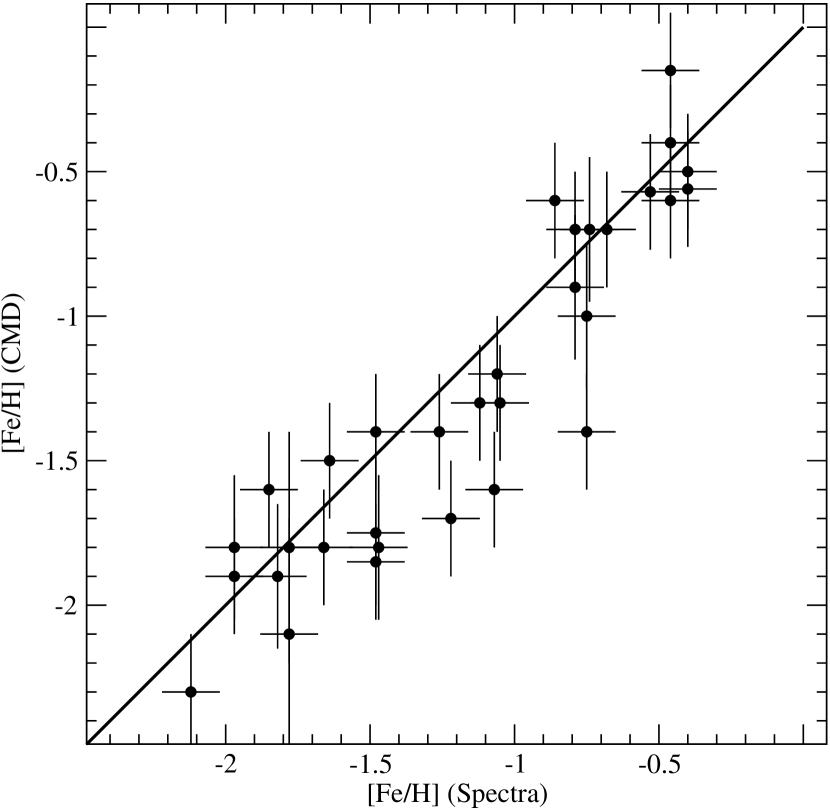
Figure 14.— Comparison of [Fe/H] derived from HST CMDs and from the spectra reported here. Clusters with more than one CMD value are shown multiple times, at the same value for [Fe/H](Spectra). The diagonal line represents equal values in the axes. The rms of the differences between the two methods is 0.2 dex.

Figure 14 shows the comparison of [Fe/H] values derived from our spectra and from CMDs either from this paper, or from the literature, for 22 clusters. These values are also listed in Table 3. Errors in the spectroscopic values are all 0.1 dex, while most of the errors in the CMD values are around 0.2 dex, except for the most metal$-$poor clusters for which we estimate the uncertainties to be 0.4 dex because the giant branch colors change slowly with metallicity. Overall the agreement is surprisingly good, given the dependence on assumed reddening for the CMD values and the uncertainties inherent in the spectroscopic values. The tendency for the middle range metallicity clusters to have higher spectroscopic estimates than those from CMDs could be due to small calibration problems with one or both of the methods The rms of the two methods is 0.2 dex.

6. Cluster Masses

Before we look further at the age and metallicity distributions, we must attend to the detail of estimating cluster masses.

6.1. New Reddenings

To estimate masses for the old clusters from the photometry in Paper I and assumed $M/L$ ratios, reddenings must be also known. Paper I described the technique used here. To repeat in brief, first the flux$-$calibrated spectra of clusters with low$-$reddening were dereddened using the Barmby et al. (2000) values. Then the spectra were ordered in metallicity, and interpolation formulae were created via a least$-$squares fit for intensity as a function of both wavelength and metallicity. This allowed a cluster spectrum of arbitrary metallicity to be formed, dereddened to the accuracy of the Barmby et al. (2000) reddenings. Reddenings for each cluster could then be found by comparing the spectra with the metallicity$-$appropriate interpolated spectrum, and adjusting reddenings as needed to bring continuum shapes close to that of the expected shape. We assumed $R_{\rm V}$=3.1, though there have been some reports that $R_{\rm V}$ is lower in M31 (Iye & Richter, 1985; Sharov & Lyutyi, 1989). Thus this method is similar to methods that used relations of metallicity and color among MW GCs to derive reddening$-$free colors of M31 clusters which had spectroscopic metallicity estimates (as was done by Barmby et al.), except that we used our flux$-$calibrated spectra to derive both the metallicities and colors.

The interpolation formulae were used to derive reddenings for the 150 GCs for which we have spectra and whose reddenings were not measured in Barmby et al. (2000), as well as to modify the reddenings that had been estimated by Barmby et al. Where we could not determine new reddenings because the spectra could not be accurately fluxed (some observations were taken with a malfunctioning ADC), we use the modal reddening of $E(B-V)$=0.13. Table Star Clusters in M31: II. Old Cluster Metallicities and Ages from Hectospec Data lists the reddenings for the clusters.

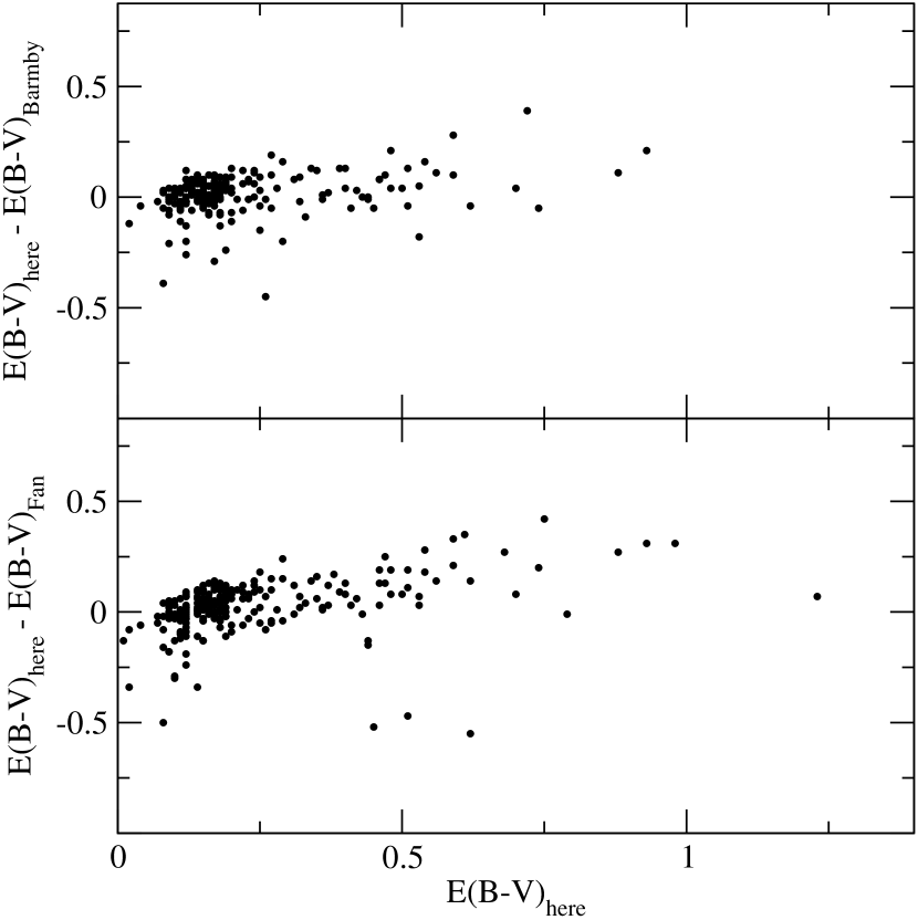
Figure 15.— Comparison with Barmby et al. (2000) and Fan et al. (2008) reddenings. The differences in reddenings determined here and by Barmby et al. (2000), top and Fan et al. (2008), bottom, are plotted against the reddenings given here in Table Star Clusters in M31: II. Old Cluster Metallicities and Ages from Hectospec Data.

Figure 15 shows a comparison of our $E(B-V)$ values with those for the same clusters contained in Barmby et al. (2000) and Fan et al. (2008). Since the Barmby et al. (2000) reddenings were used as the starting point, it is not surprising that there is no mean offset, but it is gratifying that the rms is small, at 0.09mag. The mode of our $E(B-V)$ values, like that of Barmby et al., is 0.13. The comparison with Fan et al. (2008) is good, except for 10 clusters where they show reddenings larger than ours by $>$ 0.5mag. These differences are not correlated with any obvious parameter such as reddening value or metallicity, so we have no explanation. Our reddenings are about 0.1 smaller than those of Fan et al. (2008) at low reddenings, and about 0.2 mag redder at reddenings around 0.6. van den Bergh (2007) reported a mean M31 foreground reddening of 0.06, and Massey et al. (2006) reported a mean reddening of 0.13 for OB associations, in fair and good accord respectively with the mode of our values. We estimate the uncertainties in our reddenings to be 0.1 mag.

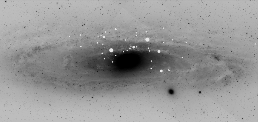
Figure 16.— Location of highly reddened clusters (image from the DSS, the diameter of the disk shown is 1.8°= 26 kpc). All white circles have reddening $E(B-V)>0.4$. Largest circles have $E(B-V)>1.2$; intermediate sized circles have reddening between 0.8 and 1.2.

Figure 16 shows the location of the most highly extincted clusters. As noted by Fan et al. (2008), these are mostly found on the NW side, which is the nearer side (the upper part in this rotated figure). B037-V327 still has the highest reddening known in M31 at $E(B-V)$=1.6, followed closely by B129 with 1.2. The former cluster actually has differential reddening across its face (Ma et al., 2006), and this is confirmed in our analysis, by the exceptionally poor correction to an unreddened spectrum. That is, using a single reddening value for the spectrum does not result in a spectrum with a continuum shape that matches other clusters with its metallicity, or any metallicity. No such problem is seen for any other cluster, thus we would state that no other cluster has significant differential reddening (though the HST image of B151-G205 shows some strong extinction in its outer parts). The reddening for B037-V327 is higher than found by Barmby et al. (2000) (1.4) and much higher than found by Strader et al. (2009) (0.92), who forced the cluster to fall on their GC fundamental plane. Our high value results in the cluster becoming the most massive cluster associated with M31, by a factor of 2.5 over the next cluster (B023-G078). Using the Barmby value still leaves it as the most massive, but brings it more in line with the other clusters.

There are 13 known MW clusters with reddenings higher than any of the known M31 clusters, which can be understood as being due to our vantage point in studying M31, not looking through its disk plane (the highest extinction MW clusters are seen at low galactic latitude). Still, it is possible that some M31 clusters remain to be found that are currently hidden behind dust lanes in the disk of M31.

6.2. Calculating the Cluster Masses

To calculate the photometric masses of the clusters, we assumed $M/L_{\rm V}$=2 independent of [Fe/H] . Stellar population models have long predicted that $M/L_{\rm V}$ should increase with [Fe/H] if age and initial mass function are fixed (Tinsley, 1980), but recently Strader et al. (2009) have shown for a small number of M31 GCs that $M/L_{\rm V}$ apparently declines with [Fe/H]. Since the matter is an active area of study, we elected to use a constant at this time and chose the value of 2 from examining the values measured in Strader et al. (2009) . The $V$ band photometry was taken from Table 1 of Paper I (obtained from images reported in Massey et al., 2006), and the reddenings from Table Star Clusters in M31: II. Old Cluster Metallicities and Ages from Hectospec Data of this paper.

Before we discuss the results, we should comment on the completeness of our catalog of M31 GCs. While we have provided much new data on the clusters contained in the catalog (including whether the catalog entry was in fact a GC), the construction of the input catalog itself was not systematic, being more of a historical document (see Caldwell et al., 2009; Galleti et al., 2007). It is likely to be nearly complete at the bright end, but the completeness at the faint end is unknown. Indeed, as we write, a new survey of the disk of M31 is being undertaken which may find many more old but low$-$mass clusters projected on the disk (HST program GO 12055, PI Dalcanton). Thus, our comments about the mass distribution here will be limited.

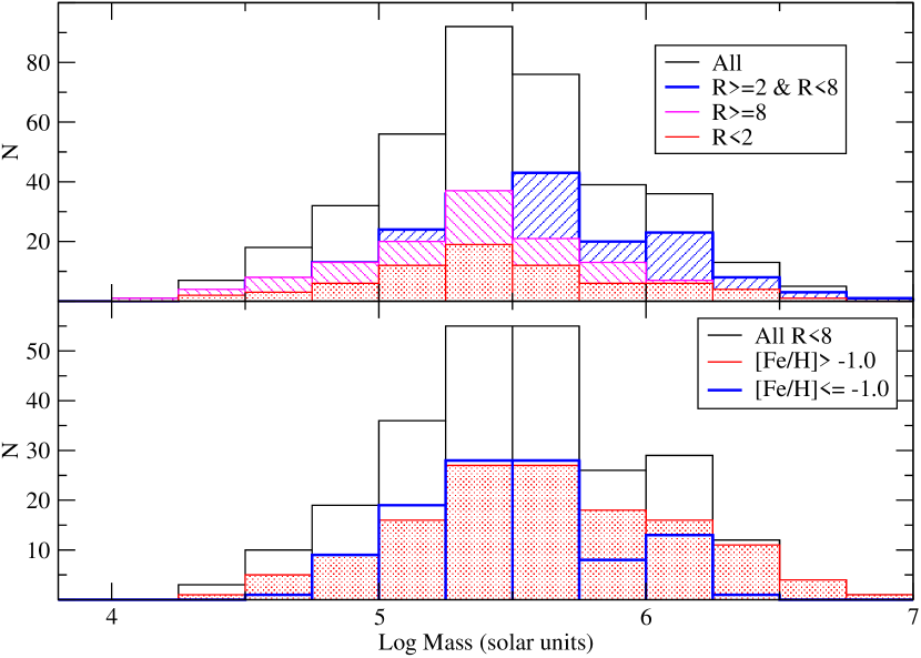
Figure 17.— Histogram of total masses of M31 GCs. Top: Clusters divided into three radial bins. Clusters inside of 8 kpc but outside of the bulge (R$>2$ kpc) tend to be more massive than those in the other two radial bins. Bottom: Clusters with R$<8$ kpc divided into two bins of metallicity. There is no obvious difference in the two mass distributions, aside of a tendency for the most and least massive clusters to be more metal-rich than [Fe/H]=$-1$.

Figure 17 shows the distribution of derived GC masses, divided into radial and metallicity bins, indicating that the masses extend from about $2\times 10^{4}$ to $10^{7}M_{\sun}$, with the most massive cluster being B037-V327 in our calculations (but see the caveat in the previous section). It is interesting that our six most massive clusters all have reddenings greater than 0.4 mag. The median cluster mass is about $3\times 10^{5}M_{\sun}$ (or $M_{\rm V}=-8.0$), which is about twice that of the MW median cluster (for which $M_{\rm V}=-7.4$, Harris, 1991). There may be a difference in the distributions when separated into mass bins, in the sense that more massive clusters tend to prefer the projected area outside of the bulge area ($R$=2 kpc) but within 8 kpc. This could be due to the most massive clusters near the bulge being destroyed. If the clusters within 8 kpc are divided in two parts at a metallicity of [Fe/H]=$-1.0$, we see another slight tendency for the metal$-$rich group to have both more massive and less massive clusters.

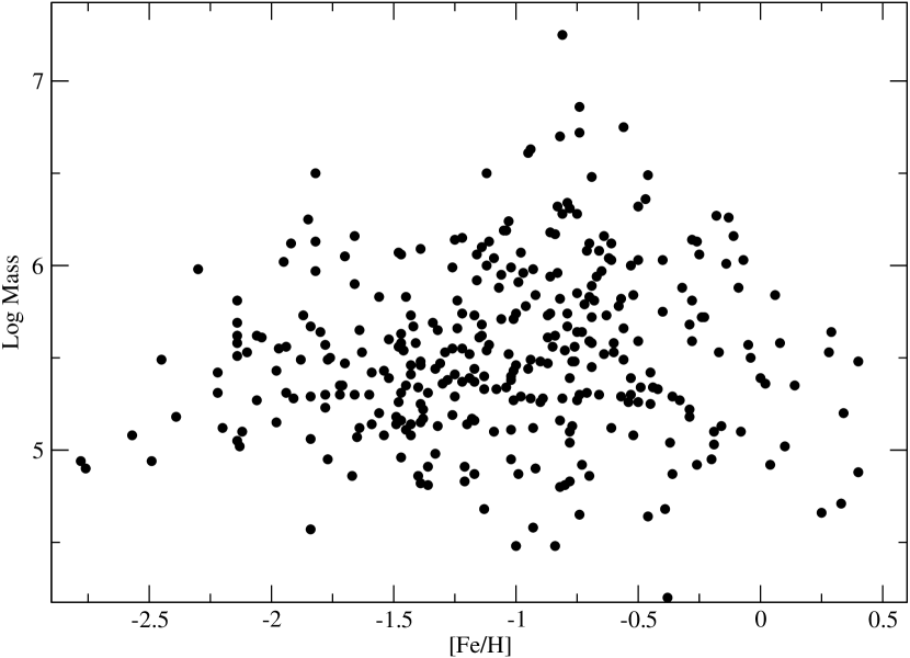
Figure 18.— Distribution of M31 clusters in the metallicity-mass plane. Mass is shown in log of solar masses. There is no evident trend of mass and metallicity for low metallicity clusters as might be expected if there was a “blue tilt” (Strader & Smith, 2008). Thus, there is no evidence for self-enrichment in the metal-poor clusters in M31.

Figure 18 shows there is no evident relation of mass and metallicity for low metallicity clusters, which might have indicated self$-$enrichment in the metal$-$poor clusters (the “blue$-$tilt”). This is in accord with Figure 21 of the Barmby et al. (2000) M31 paper. Strader & Smith (2008) noted that such a relation is not seen for MW clusters either, though it is common in early type galaxies (Harris, 2009). This figure also demonstrates that the most metal$-$rich clusters are not the most massive.

7. Discussion of Ages

We now discuss the issue of age variations among the M31 globular clusters, comparing the results found using EZ_Ages and the statements of previous authors that a number of M31 clusters have intermediate ages.

Based on archival spectra, Beasley et al. (2005) stated that, in particular, B158-G213 and B337-G068 had similar metallicities but different ages. They also stated that five M31 clusters were intermediate in age, with ages between 2 and 5Gyr: B126-G184, B301-G022, NB16, NB67 and also, B337-G068. Brodie & Strader (2006) compared the spectrum of NB67 with two other M31 clusters and concluded that it was an intermediate age cluster. Our response to those claims follows. From the Hectospec data in Table Star Clusters in M31: II. Old Cluster Metallicities and Ages from Hectospec Data, we found that (a) B158-G213 and B337-G068 are old and have dissimilar metallicities ($-0.8$ and $-1.2$, respectively), (b) B126-G184, B301-G022, NB16, and B337-G068 are all older than 9 Gyr, with [Fe/H] values ranging from $-0.8$ to $-1.5$. As it turns out, NB67 is a foreground F star (Caldwell et al., 2009). Using at the time fresh data, Burstein et al. (2004) additionally claimed that B232-G286 and B311-G033 had ages of 5 Gyr. We found that both of these clusters are old, and simply very metal$-$poor ( [Fe/H] = $-2.0$ and $-1.9$, respectively). In general, previous authors have mistaken lower metallicity clusters for younger ones. To demonstrate our claim graphically, Figure 19 highlights the six purportedly intermediate age clusters in the $\langle$Fe$\rangle$$-$H$\beta$ index diagram, similar to the top panel of Figure 9. If these clusters were substantially younger than the mean cluster age at any given metallicity (as measured by $\langle$Fe$\rangle$), we would expect them to have H$\beta$ indices stronger than the mean H$\beta$ index. Such is not the case.

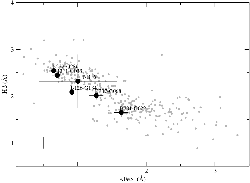
Figure 19.— $\langle$Fe$\rangle$ (average of Lick indices Fe5270 and Fe5335) plotted against H$\beta$. All of the old clusters are plotted in small, gray filled circles. The six clusters previously reported to be intermediate age are shown as large black circles, with their names attached. None of these shows any evidence for enhanced H$\beta$ strength, and hence none has evidence for an intermediate age. Average error bars for all the clusters are again shown in the bottom left corner.

A series of papers using the BATC photometric system combined with other photometry has produced several tables of ages for clusters, young and old (Fan et al., 2006; Ma et al., 2009; Wang et al., 2010). The ages were derived using SSP models, based on Padova isochrones. There is very little correlation of the ages in those papers and those we have reported here and in Paper I. The main source of the discrepancy is that many of the clusters identified by the cited papers as being young are in fact old and metal$-$poor. Of the 77 clusters in common with Wang et al. (2010), 50 clusters stated to be younger than 5 Gyr are older than 10 Gyr based on our analysis.

Returning to our own age determinations, we note again that from the EZ_Ages analysis, some clusters marked as old in Paper I were realized to be younger than 2 Gyr after publication of that paper. These are all disk clusters; Table 2 lists these clusters with their revised ages, all under 2 Gyr, as derived from the method of Paper I and confirmed by EZ_Ages. Aside of those, there are a small number of clusters (12) with ages younger than 8 and older than 2 Gyr, but six of these have abundances close to the problem [Fe/H] value of $-0.95$ and whose ages are thus suspect (see above). Thus only six are worth further consideration with regard to intermediate ages. These are B015, B071, B138, B140, B268, and AU010. Their ages are all around 7 Gyr, and all but B015 are within 2 kpc of M31’s center. These have masses between $10^{5}$ and $4\times 10^{5}M_{\sun}$, close to the median mass for all the M31 GCs. Interestingly, they are all metal$-$rich (five out of the six have [Fe/H] $>-0.2$, and have very strong CN bands.

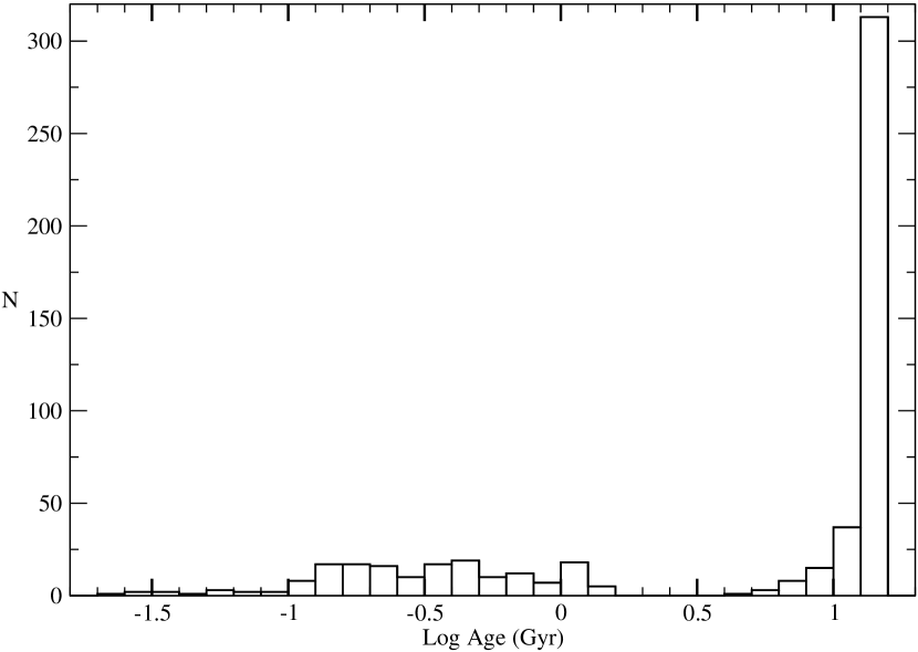
Figure 20.— Histogram of ages. Ages for clusters older than 1 Gyr were determined via EZ_Ages, ages for younger clusters come from Caldwell et al. (2009). Ages for old clusters with [Fe/H]$<-0.95$ were set to 14 (1.15 in the log).

To conclude the age discussion, we find no evidence for any massive clusters in M31 with intermediate ages, those between 2 and 6 Gyr. Figure 20 shows the age histogram, including the young clusters whose ages were determined in Paper I. For this diagram, we assumed that all clusters with [Fe/H] $<-0.95$ (whether we determined the metallicity here or others did so elsewhere) have ages of 14 Gyr. We also required the clusters to have masses greater than $5\times 10^{3}M_{\sun}$. This diagram clearly shows the gap in ages between 2 and 6 Gyr. Moreover, we have found that the mean ages of the old GCs in M31 seem to be remarkably constant over about a decade in metallicity ($-0.95\buildrel<\over{\sim}$ [Fe/H]$\buildrel<\over{\sim}0.0$).

8. M31 GC Metallicity Distribution

Next, we discuss the distribution of metal abundances for the entire M31 GC sample. For clusters we did not observe with Hectospec, we have drawn [Fe/H] values from the literature, but only when [Fe/H] values were derived from CMDs. Huxor et al. (2008) supplied 14 values for their distant sample, and 4 others came from other sources. These are G001, B468, B358-G219 (Fusi Pecci et al., 1996), and B293-G011 (Rich et al., 2005). By including these other clusters, we have expanded the discussion radius out to 100 kpc, though unfortunately many of the distant clusters do not yet have published, accurate [Fe/H] values (25 out of 38).

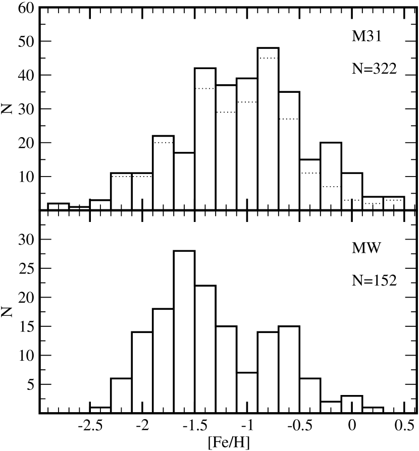
Figure 21.— Comparison of metallicity distributions for 322 M31 globulars mostly derived from spectra here (top panel), and for 152 Milky Way globulars, for which the metallicity sources are described in the text (bottom panel). The dotted histogram in the M31 panel shows that the distribution changes very little if clusters with a distance of less than 2 kpc from M31’s center are excluded.

Figure 21 shows the distribution in [Fe/H] for the 322 M31 clusters where the estimated error in [Fe/H] is less than 0.5 dex or the spectral S/N is greater than 20. We do not show clusters associated with NGC 205 here, since they are still bound to that galaxy. The distribution is not generally bimodal, because of the lack of a strong minimum, rather it shows a broad peak, centered at [Fe/H]=$-1$ . A Kolmogorov$-$Smirnoff test indicates that the observed distribution has a 28% chance of being drawn from a single Gaussian distribution, with mean [Fe/H]=$-1.08$ and sigma=0.61. (By contrast, the MW distribution has essentially no chance of coming from a single Gaussian.) To be clear, we are not stating that the distribution is unimodal, rather we find the distribution not to be clearly bimodal. Visually, the observed distribution could also contain two equal sized Gaussian distributions centered at [Fe/H]=$-0.7$ and $-1.4$, for instance, and possibly a third peak at [Fe/H]=$-0.2$, though such interpretations can not be verified statistically. A mixture$-$model KMM test (Ashman et al., 1994) of two and three peaks, with either homo$-$ or heteroscedastic variances reveals that such multimodes are not statistically significant. If we consider only the 257 clusters outside of the bulge area (roughly those farther than 2 kpc from the center), the peaks at [Fe/H]=$-0.7$ and $-1.4$ become visually slightly more prominent, though the KMM test still shows no significance to them. Also, even with that artificial restriction, there is certainly no indication that the M31 metal$-$poor peak is similar in strength or in location to the MW metal$-$poor peak at [Fe/H]$=-1.6$ (bottom panel of Figure 21).

The [Fe/H] distribution obtained from the Mg b index does show a somewhat more definite peak in the M31 clusters at $-1.4$ (Figure 8), still more metal$-$rich than the MW metal$-$poor peak. By further inspection, we found that all of the line indices that have strongly bimodal distributions also have inflections in the index versus [Fe/H] relation at low metallicity (between [Fe/H] $-1.7$ and $-1.2$, varying from index to index). The inflection is responsible for the piling up of low$-$metallicity clusters at constant index values, which leads to the low$-$metallicity peak in the index histograms (low values for metal indices, high values for Balmer indices). Therefore, the low$-$metallicity peak in those index histograms does not translate into a corresponding low$-$metallicity peak, but is rather a by$-$product of the index$-$[Fe/H] relation, which is such that metal$-$poor clusters in a wide range of metallicities have approximately the same index values.

Whether a peak at [Fe/H]=$-1.4$ is real or not will require better calibration than we currently have, in particular more metal$-$poor MW GCs are necessary. We maintain that our $\langle$Fe$\rangle$$-$[Fe/H] method is the best one to use $-$ previous calibrations used stronger lines, and even less data to calibrate the MW GCs $-$ but the calibration here must still be seen as preliminary, and thus the M31 [Fe/H] distribution is not yet firmly established, though we are much closer than previously. The M31 GC metallicity distribution is definitely different from the MW GC distribution, and certainly it is not simple to divide the clusters into two groups as has been done for the MW GCs. This fact must indicate that the formation of the M31 cluster system was substantially different from that in the MW.

8.1. Comparison with MW GCs

In order to compare the metallicities of M31’s old clusters with the Milky Way’s, we took the MW cluster data originally compiled by Harris (1991), and subsequently updated by Bica et al. (2006), and further updated it with 17 new metallicities of Carretta et al. (2009). This results in values for 152 MW clusters, whose distribution is shown below that of the M31 clusters in Figure 21, indicating the well$-$known peaks at [Fe/H]=$-1.6$ and $-0.6$ (e.g., Bica et al., 2006).

It is interesting to note that Huchra et al. (1991) presented a metallicity distribution for the M31 globulars which was quite similar to the Milky Way’s, prompting the comment “Like the Milky Way, only more so.” We do not find this to be the case. The modal metallicity in their M31 histograms was quite low, near [Fe/H]=$-1.7$. As more clusters which were projected on the disk were studied, the modal metallicity moved higher, to $-1.3$ (Barmby et al., 2000) and then to $-1.1$ (Perrett et al., 2002). Both our measurement and that of Galleti et al. (2009), based on metallicities found in the literature prior to this paper, agree on a modal metallicity that is actually higher than [Fe/H]=$-1.0$. Ashman & Bird (1993) derived a bimodal metallicity distribution using the data of Huchra et al. (1991), and Barmby et al. (2000) reported marginal confirmation of bimodality using $U-V$, $U-R$ and $V-K$ colors (marginal in the sense that bimodality was found at the 92$-$95% confidence level). Fan et al. (2008) used literature spectroscopic metallicity values and newly derived metallicities from colors and also derived a bimodal M31 GC metallicity distribution (significant at a level greater than 95%). However, all of those studies suffered from the inclusion of clusters now thought to be young, which may explain in part why those studies found more significance to bimodality. An additional factor must be the conversion of colors to metallicity (Yoon et al., 2006), which is non$-$linear at the metal$-$poor end, leading to further difficulties interpreting bimodality.

It has been known for some time (see, for example Mould & Kristian, 1986) that the field stars in M31’s halo are significantly more metal$-$rich than the MW halo’s field stars. This, combined with the early results on the M31 cluster metallicity distribution being similar to the MW clusters, prompted Durrell et al. (1994) to point out that there was a curious offset between the M31 halo cluster and field metallicities. Freeman (1996) suggested that perhaps the $R^{1/4}$ bulge contributed significantly to the halo field (but not the globular clusters) at large distances from its center. However, it now seems that the metallicity distribution of old clusters in M31 is also relatively metal$-$rich, removing the need for such distinctions.

What of the extremes of the distribution? Do we have evidence that the globulars in M31 have metallicities that reach higher or lower than the MW system? The M31 cluster distribution does apparently extend further to the metal$-$rich and metal$-$poor ends than the MW’s, but for the metal$-$poor end the most we can say is that there are M31 clusters as metal$-$poor as those in the MW, such as NGC7089 (which has [Fe/H]=$-2.4$). Our technique of using only Fe indices to measure [Fe/H] has a natural failing at the metal$-$poor end because of the decreasing S/N of those features, which is compounded by the break in the relation of the Lick Fe indices and [Fe/H] for MW clusters (see Figure 7). The clusters B157-G212 and B028-G088 have very high S/N spectra and are definitely as metal$-$poor as NGC7089, but whether they are more metal$-$poor as our table indicates would require higher spectral resolution data or individual star spectra.

However, there are several M31 old clusters with [Fe/H] greater than solar and low measurement errors. Such super$-$metal$-$rich globulars are not seen in the MW. While previously it was possible to suppose that these clusters existed in the MW but were hidden by dust extinction, both the 2MASS and GLIMPSE surveys have only identified a handful of new clusters. This means that our catalog of MW GCs is close to complete. It is likely that we are seeing a real difference in the metallicity distributions at the metal$-$rich end, perhaps caused by the significantly larger number of M31 old clusters. By contrast, the absence of strong evidence for more metal$-$poor clusters in M31 (added to the dearth of clusters with metallicity less than $-$2.5 in the LMC, Sgr and Fornax dwarfs, Mackey & Gilmore, 2004) hints that there is some physical mechanism which prevents the formation of extremely metal$-$poor globular clusters.

The other obvious difference between the metallicity distributions of M31 and MW GCs is the bimodality in the Milky Way distribution, which has been known for some time. In an influential early paper, Zinn (1985) pointed out the clear division of the globular clusters into two systems, which he named the halo and disk clusters. This division can be seen clearly in a number of different properties of the clusters. First, MW disk clusters have small distances from both the galactic center and the galactic plane while halo clusters extend out to large values of both. Second, the MW disk GCs are on the metal$-$rich side of the metallicity distribution, having [Fe/H]$>-0.8$, and the halo clusters are of course metal$-$poor. Finally, the disk globulars are rotationally supported, although they have hotter kinematics than the Galaxy’s thin disk, while the halo globulars have a mean rotation close to zero and a high velocity dispersion.

Minniti (1995) and Côté (1999) later suggested that the metal$-$rich clusters are associated with the galactic bulge or perhaps the bar. Others have proposed divisions into young halo, old halo, bulge/disk (Mackey & van den Bergh, 2005; Fraix-Burnet et al., 2009) based on numerous observed properties of the clusters.

While the M31 globulars do not have a clearly bimodal metallicity distribution, it is interesting to examine the variation of metallicity with position in M31. Because we do not have 3$-$D positions of our clusters in M31, we cannot simply plot [Fe/H] against $z$ distance to make comparisons with Zinn’s results; but because M31 is quite highly inclined to the line of sight, we can reasonably use the distance from the major axis, Y, as a proxy.

Figure 22.— Relation between metallicity and position in M31. In the top panel we show the variation of [Fe/H] with log(radius), and in the bottom panel with the log of the minor axis distance Y, which is the closest comparison we can make to the 3-D distance above or below the galactic mid-plane. The dotted line in the bottom panel marks [Fe/H]= $-0.4$. Clusters with higher metallicities than this appear to be confined to distances close to the midplane.

We can contrast the spatial and chemical properties of the two old cluster systems by examining Figure 22, which plots both projected radial distance from M31’s center and the minor axis distance Y against [Fe/H]. We see that M31 shows marked similarities to the MW populations first noted by Zinn, with some intriguing differences. We see that, as in the MW, the most metal$-$rich clusters in M31 are restricted to its inner regions, both in radius and in minor axis distance, which is our best proxy for height above the plane. Conversely, the more metal$-$poor clusters occupy a large range in radial and minor$-$axis distance. However, in M31 it is only the clusters with [Fe/H] greater than $-0.4$ (see the dotted line in the bottom panel) which are confined to distances close to the midplane. M31 clusters with [Fe/H] greater than $-0.4$ have a median $|$Y$|$ distance of 1 kpc, while clusters with [Fe/H] less than $-0.4$ have a median $|$Y$|$ distance of 2 kpc. We also see a hint of a new feature: a third break around [Fe/H]=$-1.5$. The outer halo clusters, which reach out to $\sim$100 kpc in projection, all have metallicities lower than $-1.5$. This is a numerically small group even in M31, and it is possible that the smaller total number of MW GCs has obscured a similar pattern. Spectroscopic metallicity measurements of these M31 far outer halo globulars will also be useful for more precise comparisons.

8.2. Radial Distribution of Clusters

The left panel of Figure 23 shows the radial distribution of all M31 and MW GCs, the latter data coming again from the compilation of Harris (1991). Projection onto the $YZ$ plane was used for MW clusters, and circular symmetry was assumed for both galaxies. The outer M31 clusters ($R>3$ kpc) follow the $-2.5$ power law seen in the MW halo stars, but the M31 GC profile is more shallow than that at smaller radii (the exponent changes to $-1.2$; overall the M31 GC profile may be fit with a Sérsic profile with index $n$=2.3). It is hard to assess the importance of the difference between the two galaxies’ profiles in the inner 3 kpc, given that these are the only two galaxies for which we have such detailed information. If the M31 clusters are divided up into three metallicity regimes as shown in the figure, we see that the metal$-$rich clusters have a gap in their distribution, with few between 2 and 5 kpc. Several of the metal$-$rich clusters in the denser region beyond 5 kpc are possibly not true globulars (e.g., the low mass clusters B186, B279-D068, B054-G115, and B522), but this represents only a quarter of the clusters in that region, and thus the gap between 2 and 5 kpc appears to be real. The gap does not appear for either of the two more metal$-$poor bins at that radius shown in the figure.

We will continue our comparisons with the MW GC system when we present the old cluster kinematics in another paper in this series (A. Romanowsky et al., 2011, in preparation).

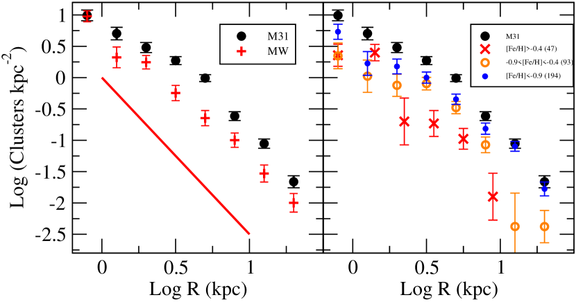
Figure 23.— Left:Radial profile of the M31 cluster system compared to that for MW clusters. Projection onto the YZ plane was used for the MW clusters. Circular symmetry was assumed for both galaxies. The solid line represents a $-2.5$ power law, which corresponds to the projected MW halo profile. Right: M31 radial profile broken up into three different metallicity bins. The dip in the metal-rich cluster distribution between log R = 0.3 and 0.7 ($2<$R$<5$ kpc) appears to be real.

9. Summary and General Comments

Using the high$-$quality spectra reported here, we have provided new homogeneous estimates of the metallicities and ages for more than 300 globular clusters in M31. Again, within a radius 21 kpc we observed 94% of the old clusters. We note that only 13% of MW GCs lie beyond that limit of 21 kpc. The search for outer M31 clusters, presumably metal$-$poor, is still underway (e.g., Huxor et al., 2008), but it is unlikely that enough clusters will be discovered to change our basic comparison of metal$-$rich and metal$-$poor clusters in M31

We find no evidence for any massive clusters in M31 with intermediate ages, those between 2 and 6 Gyr.

The metallicities span the range of those found in the MW, with a few clusters perhaps extending beyond the most metal$-$rich galactic globulars. The M31 cluster metallicity distribution is quite different from that of the MW, not showing a strong bimodality as does the MW. However, there are hints of multi$-$modality. Since it is likely that GCs were deposited in M31 in a hierarchical fashion from merging and accretion of a number of smaller galaxies, the lack of simple bimodality in the M31 cluster [Fe/H] distribution is perhaps not surprising.

Our new data confirm about 320 true GCs. To that we may add another 50 clusters which we did not observe, but which have been confirmed as globulars by various sources, but most significantly by Barmby et al. (2000) and Huxor et al. (2008). Thus the total number of known M31 GCs is about 370, compared with 150 for the MW (Harris, 1991). We close this paper with some other comparisons between the two galaxies.

Roughly, in M31 the metal$-$poor and metal$-$rich groups have equal numbers of clusters. There are 333 clusters with [Fe/H] measured here or in the literature. If we divide them at [Fe/H]=$-1$, there are 160 above that with a combined mass of $1\times 10^{8}M_{\sun}$ and 173 below it with a mass of $8\times 10^{7}M_{\sun}$. If we place all the clusters with unmeasured [Fe/H] into the metal$-$poor group (there are 39 of these, mostly in the outer halo), the result changes only slightly. There would be 218 clusters in the metal$-$poor group, but the total mass increases only to $9\times 10^{7}M_{\sun}$ since most of the added clusters are low mass. In the MW, that same dividing point in [Fe/H] divides the clusters into 1/3 metal$-$rich and 2/3 metal$-$poor, with the former having a total mass of $9\times 10^{6}M_{\sun}$ and the latter with $3\times 10^{7}M_{\sun}$.

The relative total masses of M31 and the MW are a topic of current interest (Reid et al., 2009), but we can limit the discussion to the bulge masses, the ratio of which is about a factor of 2 (van der Kruit, 1990). Therefore, the ratio of number of GCs of all metallicities to the parent’s bulge mass does appear to be similar in the two galaxies. However, the ratio of the numbers of metal$-$rich GCs to bulge mass, or equivalently, the ratio of metal$-$poor clusters to the bulge mass is not similar, due implicitly to the different ratio of metal$-$rich to metal$-$poor clusters between M31 and the MW.

The specific frequency of GCs is defined as the ratio of the number of clusters of all metallicity to the galaxy luminosity in units of $M_{\rm V}=-15$. Since M31 has about 370 GCs, and has $M_{\rm V}=-21.2$ (van den Bergh, 2007), we then find a specific frequency of 1.2. Isolating the bulge luminosity (taken to be 30% of the total light), we derive a bulge specific frequency of 4. These numbers can be compared with the values of 1 and 2 for the MW (the latter for the bulge specific frequency. Thus, M31 has more clusters per unit luminosity of old stars.

In M31, 50% of the known GCs lie within 5.1 kpc of the Galactic center, remarkably close to the half$-$total number radius of 4.8 kpc for the MW. (We calculated the projected radius of the MW GCs in the $YZ$ plane). However, the half$-$mass radius of the M31 GC system is smaller, 3.7 kpc, because the more distant clusters are less massive in the mean than the inner ones. The half$-$mass radius for the MW GC system is about 5.5 kpc, slightly larger than the half$-$total number radius.

Succeeding papers in this series will concentrate on the abundance ratios of the clusters, the relation of kinematics and abundances in the cluster system, the horizontal branch morphologies, and the $M/L$ ratios of the clusters as derived from high dispersion spectroscopy and HST imaging.

Table 1Results from the Spectra of Old M31 Clusters

Object	RA	Dec	$E(B-V)$	Velocity	Log Mass	[Fe/H]	Age	notes
	J2000			km s-1	M☉		Gyr
B291-G009	0:36:04.97	42:02:09.3	0.12	$-$213.5$\pm 14$	5.5	$-$1.2$\pm 0.1$	(14)
B295-G014	0:36:46.73	40:19:42.1	0.03	$-$415.3$\pm 26$	5.3	$-$1.7$\pm 0.2$	(14)
B422	0:37:38.45	41:59:59.2	0.09	$-$202.4$\pm 18$	4.9	$-$1.2$\pm 0.2$	(14)
B301-G022	0:38:21.59	40:03:37.0	0.19	$-$366.6$\pm 7$	5.5	$-$0.9$\pm 0.1$	(14)
B167D	0:38:22.48	41:54:35.0	0.11	$-$196.4$\pm 15$	5.0	$-$1.5$\pm 0.2$	(14)
B302-G023	0:38:33.5	41:20:52.2	0.05	$-$394.4$\pm 22$	5.4	$-$1.5$\pm 0.3$	(14)
MCGC7-H14	0:38:49.39	42:22:47.0	(0.13)	$-$247.6$\pm 25$	4.9	$-$0.7$\pm 0.7$	(14)
B304-G028	0:38:56.94	41:10:28.4	0.14	$-$405.3$\pm 15$	5.4	$-$1.3$\pm 0.1$	(14)
B306-G029	0:39:08.70	40:34:21.2	0.57	$-$443.9$\pm 9$	6.1	$-$1.1$\pm 0.1$	(14)
B309-G031	0:39:24.62	40:14:29.1	0.20	$-$404.3$\pm 16$	5.3	$-$1.2$\pm 0.2$	(14)
B310-G032	0:39:25.75	41:23:33.1	0.13	$-$238.1$\pm 14$	5.3	$-$1.4$\pm 0.1$	(14)
B181D	0:39:30.85	41:28:26.4	0.03	$-$203.7$\pm 8$	5.0	$-$1.0$\pm 0.1$	(14)
B311-G033	0:39:33.72	40:31:14.7	0.36	$-$523.4$\pm 20$	6.2	$-$1.9$\pm 0.2$	(14)
B312-G035	0:39:40.17	40:57:02.4	0.23	$-$177.5$\pm 9$	6.1	$-$1.2$\pm 0.1$	(14)
B313-G036	0:39:44.60	40:52:55.2	0.39	$-$429.5$\pm 8$	5.9	$-$1.0$\pm 0.1$	(14)
B001-G039	0:39:51.02	40:58:10.6	0.39	$-$203.3$\pm 8$	5.7	$-$0.7$\pm 0.1$	11.9
B317-G041	0:39:55.29	41:47:45.9	0.12	$-$178.2$\pm 16$	5.5	$-$2.1$\pm 0.2$	(14)
B002-G043	0:40:02.57	41:11:53.5	0.11	$-$338.2$\pm 14$	5.1	$-$2.2$\pm 0.2$	(14)
B003-G045	0:40:09.40	41:11:05.6	0.12	$-$377.0$\pm 11$	5.1	$-$1.6$\pm 0.2$	(14)
B004-G050	0:40:17.92	41:22:40.2	0.18	$-$369.8$\pm 6$	5.5	$-$0.7$\pm 0.1$	12.2
B005-G052	0:40:20.33	40:43:58.3	0.16	$-$291.6$\pm 9$	5.9	$-$0.7$\pm 0.1$	(14)
B328-G054	0:40:24.52	41:40:23.1	0.16	$-$281.5$\pm 13$	5.2	$-$1.2$\pm 0.2$	(14)	e
B330-G056	0:40:25.58	41:42:53.6	0.12	$-$247.3$\pm 17$	5.1	$-$1.4$\pm 0.1$	(14)
B331-G057	0:40:26.10	41:42:03.9	0.06	$-$242.9$\pm 8$	4.8	$-$0.8$\pm 0.2$	5.3
B006-G058	0:40:26.48	41:27:26.7	0.17	$-$232.4$\pm 6$	6.0	$-$0.5$\pm 0.1$	(14)
B244	0:40:26.49	41:18:35.5	0.10	$-$237.8$\pm 13$	4.8	$-$1.4$\pm 0.2$	(14)
BH04	0:40:27.2	41:42:23.9	0.06	$-$224.6$\pm 22$	4.2	$-$0.4$\pm 0.6$	(14)
B333	0:40:29.58	41:40:26.7	0.10	$-$239.3$\pm 8$	4.5	$-$0.8$\pm 0.2$	5.3
B008-G060	0:40:30.28	41:16:08.7	0.20	$-$318.0$\pm 4$	5.6	$-$0.8$\pm 0.1$	13.5
B009-G061	0:40:30.70	41:36:55.6	0.10	$-$294.9$\pm 10$	5.4	$-$1.3$\pm 0.1$	(14)
B010-G062	0:40:31.56	41:14:22.5	0.19	$-$164.4$\pm 10$	5.6	$-$1.8$\pm 0.2$	(14)
B011-G063	0:40:31.87	41:39:16.9	0.10	$-$237.8$\pm 13$	5.4	$-$1.2$\pm 0.1$	(14)
B012-G064	0:40:32.46	41:21:44.2	0.17	$-$355.7$\pm 11$	6.2	$-$1.7$\pm 0.1$	(14)
B013-G065	0:40:38.43	41:25:23.7	0.17	$-$411.5$\pm 6$	5.3	$-$0.5$\pm 0.1$	9.5
B015-V204	0:40:45.02	40:59:56.3	0.58	$-$460.0$\pm 7$	5.6	$-$0.1$\pm 0.2$	7.2
B016-G066	0:40:45.16	41:22:09.9	0.27	$-$388.4$\pm 5$	5.3	$-$0.7$\pm 0.1$	11.1
B336-G067	0:40:47.60	42:08:43.2	0.05	$-$609.0$\pm 27$	4.9	$-$2.5$\pm 0.6$	(14)
B337-G068	0:40:48.47	42:12:11.0	0.10	$-$278.5$\pm 14$	5.4	$-$1.2$\pm 0.1$	(14)
B017-G070	0:40:48.73	41:12:07.1	0.47	$-$530.4$\pm 6$	6.2	$-$0.8$\pm 0.1$	11.8
B246	0:40:52.29	40:53:55.9	0.08	$-$496.8$\pm 13$	4.7	$-$0.7$\pm 0.3$	(14)
B019-G072	0:40:52.52	41:18:53.8	0.22	$-$220.4$\pm 6$	6.3	$-$0.8$\pm 0.1$	10.9
B020-G073	0:40:55.26	41:41:25.2	0.11	$-$345.4$\pm 5$	6.2	$-$0.9$\pm 0.1$	8.6
B338-G076	0:40:58.87	40:35:47.9	0.15	$-$275.8$\pm 12$	6.5	$-$1.1$\pm 0.1$	(14)
B021-G075	0:40:58.99	41:05:39.1	0.56	$-$419.1$\pm 7$	5.6	$-$0.5$\pm 0.1$	12.6
B022-G074	0:40:59.08	41:24:42.0	0.14	$-$454.4$\pm 11$	5.2	$-$1.8$\pm 0.2$	(14)
B339-G077	0:41:00.71	39:55:54.2	(0.13)	$-$227.1$\pm 13$	5.4	$-$0.5$\pm 0.2$	(14)
B023-G078	0:41:01.19	41:13:45.7	0.42	$-$443.9$\pm 7$	6.9	$-$0.7$\pm 0.1$	11.8
B248	0:41:07.94	40:53:01.0	0.30	$-$570.3$\pm 10$	5.2	$-$1.4$\pm 0.2$	(14)
B341-G081	0:41:09.15	40:35:52.8	0.20	$-$364.9$\pm 8$	5.7	$-$0.9$\pm 0.1$	12.4
B024-G082	0:41:11.86	41:45:49.1	0.19	$-$215.0$\pm 5$	5.5	$-$0.6$\pm 0.1$	(14)
B025-G084	0:41:12.55	41:00:28.3	0.35	$-$204.9$\pm 15$	5.7	$-$1.4$\pm 0.1$	(14)
B249	0:41:12.58	41:01:12.7	0.37	$-$536.7$\pm 9$	5.2	0.3$\pm 0.2$	8.5
B027-G087	0:41:14.54	40:55:50.9	0.19	$-$302.9$\pm 16$	6.0	$-$1.3$\pm 0.1$	(14)
B026-G086	0:41:14.55	41:24:40.1	0.28	$-$250.8$\pm 5$	5.3	$-$0.4$\pm 0.1$	(14)
B028-G088	0:41:16.50	40:59:03.2	0.20	$-$414.2$\pm 19$	5.5	$-$2.5$\pm 0.2$	(14)
B020D-G089	0:41:17.23	41:08:09.1	0.49	$-$558.0$\pm 17$	5.6	$-$2.1$\pm 0.2$	(14)
B029-G090	0:41:17.82	41:00:23.0	0.27	$-$500.0$\pm 7$	5.7	$-$0.3$\pm 0.1$	13.4
B030-G091	0:41:18.74	40:57:15.6	0.65	$-$390.9$\pm 6$	5.9	$-$0.3$\pm 0.1$	(14)
B031-G092	0:41:20.93	40:59:04.2	0.31	$-$310.8$\pm 8$	5.3	$-$0.5$\pm 0.1$	11.5
B032-G093	0:41:21.51	41:17:30.2	0.51	$-$526.3$\pm 7$	5.6	$-$0.7$\pm 0.1$	12.3
B033-G095	0:41:26.40	41:00:14.0	0.30	$-$466.5$\pm 16$	5.3	$-$1.6$\pm 0.3$	(14)
B034-G096	0:41:28.12	40:53:49.6	0.16	$-$556.5$\pm 10$	6.0	$-$0.6$\pm 0.1$	(14)
B457-G097	0:41:29.23	42:18:37.1	0.13	$-$330.0$\pm 18$	5.4	$-$1.1$\pm 0.2$	(14)
B035	0:41:32.58	41:38:32.7	0.21	$-$45.7$\pm 5$	5.3	$-$0.8$\pm 0.1$	11.7
B036	0:41:32.83	41:26:05.1	0.25	$-$506.2$\pm 6$	5.4	$-$0.8$\pm 0.1$	(14)
B037-V327	0:41:34.98	41:14:55.1	1.61	$-$322.8$\pm 11$	7.2	$-$0.8$\pm 0.1$	(14)
B038-G098	0:41:35.95	41:19:14.8	0.40	$-$183.4$\pm 9$	5.9	$-$1.7$\pm 0.1$	(14)
B039-G101	0:41:37.87	41:20:50.1	0.60	$-$246.6$\pm 6$	6.3	$-$0.8$\pm 0.1$	9.0
B041-G103	0:41:40.81	41:14:45.4	(0.13)	$-$398.2$\pm 2$	4.7		(14)
B042-G104	0:41:41.69	41:07:26.2	0.88	$-$293.8$\pm 12$	6.6	$-$0.9$\pm 0.1$	6.7
B044-G107	0:41:42.91	41:20:06.2	0.47	$-$267.6$\pm 6$	5.8	$-$0.8$\pm 0.1$	13.3
B343-G105	0:41:43.10	40:12:22.4	0.15	$-$356.0$\pm 14$	5.7	$-$1.6$\pm 0.2$	(14)
B045-G108	0:41:43.11	41:34:20.3	0.18	$-$419.4$\pm 6$	5.9	$-$0.9$\pm 0.1$	(14)
B046-G109	0:41:44.60	41:46:27.7	0.18	$-$351.3$\pm 7$	5.1	$-$1.1$\pm 0.1$	(14)
B048-G110	0:41:45.53	41:13:30.6	0.36	$-$234.6$\pm 10$	5.8	$-$0.8$\pm 0.1$	(14)
B047-G111	0:41:45.56	41:42:04.1	0.16	$-$294.8$\pm 9$	5.2	$-$1.6$\pm 0.2$	(14)
B050-G113	0:41:46.28	41:32:18.7	0.25	$-$109.5$\pm 6$	5.6	$-$0.8$\pm 0.1$	13.5
B051-G114	0:41:46.70	41:25:19.1	0.38	$-$261.2$\pm 6$	6.0	$-$0.8$\pm 0.1$	(14)
B054-G115	0:41:47.68	41:00:55.3	0.17	$-$397.2$\pm 8$	5.0	$-$0.2$\pm 0.1$	10.6
B055-G116	0:41:50.39	41:12:12.4	0.54	$-$304.9$\pm 8$	6.0	$-$0.1$\pm 0.1$	(14)
B254	0:41:50.5	41:16:25.9	0.29	$-$421.0$\pm 12$	4.9	$-$0.9$\pm 0.2$	4.8
B522	0:41:50.95	40:52:48.2	0.11	$-$390.2$\pm 23$	4.7	$-$0.4$\pm 0.6$	9.1	e
B056-G117	0:41:51.16	40:57:40.2	0.24	$-$363.7$\pm 7$	5.4	$-$0.0$\pm 0.1$	(14)
B057-G118	0:41:52.82	40:52:05.1	0.10	$-$411.1$\pm 21$	5.1	$-$2.1$\pm 0.3$	(14)
B058-G119	0:41:53.00	40:47:09.7	0.15	$-$220.2$\pm 11$	6.2	$-$1.1$\pm 0.1$	(14)
B059-G120	0:41:54.11	41:11:00.7	0.49	$-$262.1$\pm 8$	5.7	$-$1.0$\pm 0.1$	(14)
B060-G121	0:41:57.01	41:05:14.5	0.13	$-$533.2$\pm 16$	5.5	$-$1.8$\pm 0.1$	(14)
B061-G122	0:42:00.14	41:29:35.7	0.49	$-$275.2$\pm 5$	6.0	$-$0.7$\pm 0.1$	(14)
B063-G124	0:42:00.88	41:29:09.5	0.49	$-$301.6$\pm 8$	6.3	$-$0.8$\pm 0.1$	13.8
B065-G126	0:42:01.93	40:40:13.1	0.17	$-$417.3$\pm 12$	5.5	$-$0.9$\pm 0.2$	(14)
B064-G125	0:42:01.93	41:11:07.5	0.17	$-$302.4$\pm 10$	5.7	$-$1.3$\pm 0.1$	(14)
B344-G127	0:42:02.97	41:52:02.2	0.13	$-$240.6$\pm 6$	5.8	$-$1.0$\pm 0.1$	(14)
B067-G129	0:42:03.19	41:04:23.7	0.08	$-$356.8$\pm 15$	5.2	$-$1.4$\pm 0.1$	(14)
B068-G130	0:42:03.21	40:58:50.2	0.45	$-$319.2$\pm 6$	6.1	$-$0.2$\pm 0.1$	(14)
B257-V219	0:42:03.28	40:58:13.9	0.66	$-$476.4$\pm 6$	5.7	$-$0.2$\pm 0.1$	(14)
B461-G131	0:42:04.24	42:03:26.6	0.10	$-$296.5$\pm 8$	5.1	$-$0.6$\pm 0.1$	13.7
B041D	0:42:04.72	41:16:47.3	0.64	$-$208.3$\pm 14$	5.5	$-$1.8$\pm 0.4$	(14)
B070-G133	0:42:06.91	41:07:56.3	0.20	$-$275.8$\pm 22$	5.6	$-$1.9$\pm 0.2$	(14)
B071	0:42:07.13	41:12:12.0	0.24	$-$550.7$\pm 8$	5.1	$-$0.2$\pm 0.2$	6.9
B073-G134	0:42:07.33	40:59:21.3	0.13	$-$504.0$\pm 10$	5.8	$-$0.6$\pm 0.1$	12.6
B072	0:42:07.44	41:22:47.6	0.78	$-$85.7$\pm 7$	5.8	$-$0.7$\pm 0.1$	12.0
B074-G135	0:42:08.04	41:43:21.6	0.16	$-$439.9$\pm 9$	5.5	$-$1.5$\pm 0.1$	(14)
B075-G136	0:42:08.83	41:20:21.3	0.32	$-$168.6$\pm 11$	5.4	$-$1.3$\pm 0.2$	(14)
MITA140	0:42:09.51	41:17:45.6	0.86	$-$319.4$\pm 12$	6.3	$-$0.2$\pm 0.1$	(14)
B045D	0:42:09.87	41:21:14.5	0.41	$-$305.9$\pm 13$	4.9	$-$0.3$\pm 0.3$	(14)
B076-G138	0:42:10.24	41:05:22.0	0.17	$-$537.0$\pm 14$	5.5	$-$1.3$\pm 0.1$	(14)
B077-G139	0:42:11.14	41:07:33.9	0.46	$-$562.8$\pm 7$	5.7	$-$0.8$\pm 0.1$	(14)	e
B078-G140	0:42:12.17	41:17:58.9	(0.43)	$-$259.7$\pm 16$	5.5	$-$1.0$\pm 0.2$	(14)
B080-G141	0:42:12.40	41:19:00.6	0.72	$-$255.0$\pm 21$	5.8	$-$1.4$\pm 0.2$	(14)
B345-G143	0:42:14.12	40:17:36.5	0.19	$-$368.4$\pm 12$	5.6	$-$1.5$\pm 0.1$	(14)
B462	0:42:14.72	42:01:36.7	0.13	$-$214.3$\pm 23$	4.9	$-$2.8$\pm 0.3$	(14)
B082-G144	0:42:15.84	41:01:14.4	0.94	$-$370.5$\pm 8$	6.7	$-$0.7$\pm 0.1$	10.3
B083-G146	0:42:16.44	41:45:20.7	0.13	$-$337.3$\pm 6$	5.3	$-$1.1$\pm 0.1$	(14)
B084	0:42:17.45	41:18:55.7	0.62	$-$325.8$\pm 10$	5.6	$-$1.1$\pm 0.2$	(14)
B085-G147	0:42:18.24	40:39:57.2	0.16	$-$425.4$\pm 12$	5.5	$-$1.7$\pm 0.2$	(14)
B086-G148	0:42:18.65	41:14:02.1	0.13	$-$189.0$\pm 19$	6.1	$-$1.8$\pm 0.2$	(14)	e
B087	0:42:19.81	41:38:16.2	0.24	$-$369.2$\pm 9$	4.9	$-$1.0$\pm 0.2$	(14)	near star
B088-G150	0:42:21.07	41:32:14.2	0.53	$-$489.9$\pm 12$	6.5	$-$1.8$\pm 0.1$	(14)
B090	0:42:21.08	41:02:57.5	0.15	$-$399.9$\pm 7$	4.8	$-$0.8$\pm 0.2$	(14)	e
B092-G152	0:42:22.38	41:08:08.7	0.11	$-$433.7$\pm 12$	5.4	$-$1.0$\pm 0.1$	(14)
B347-G154	0:42:22.89	41:54:27.5	0.02	$-$266.4$\pm 26$	5.4	$-$2.0$\pm 0.2$	(14)
B348-G153	0:42:22.92	41:52:28.4	0.16	$-$189.5$\pm 7$	5.5	$-$0.8$\pm 0.1$	(14)
B093-G155	0:42:23.17	41:21:43.5	0.39	$-$456.7$\pm 22$	5.7	$-$1.2$\pm 0.1$	(14)
B094-G156	0:42:25.06	40:57:17.7	0.22	$-$564.1$\pm 6$	6.0	$-$0.4$\pm 0.1$	(14)
B095-G157	0:42:25.80	41:05:36.3	0.46	$-$111.2$\pm 10$	6.1	$-$1.4$\pm 0.1$	(14)
B096-G158	0:42:26.1	41:19:14.8	0.63	$-$313.4$\pm 8$	6.1	$-$0.3$\pm 0.1$	(14)
B098	0:42:27.40	40:59:36.1	0.19	$-$308.6$\pm 9$	5.7	$-$0.8$\pm 0.1$	8.7
B097-G159	0:42:27.48	41:25:32.1	0.34	$-$272.1$\pm 8$	5.7	$-$1.0$\pm 0.1$	(14)
B099-G161	0:42:27.59	41:10:02.7	0.16	$-$108.1$\pm 10$	5.5	$-$1.3$\pm 0.1$	(14)
B515	0:42:28.05	41:33:24.5	(0.13)	$-$276.7$\pm 2$	4.7		(14)
B056D	0:42:28.36	41:34:27.2	(0.13)	$-$188.0$\pm 12$	4.8			r
B350-G162	0:42:28.44	40:24:51.1	0.12	$-$423.9$\pm 12$	5.5	$-$1.4$\pm 0.1$	(14)
B100-G163	0:42:28.96	40:49:56.0	0.15	$-$428.4$\pm 8$	5.1	$-$0.9$\pm 0.1$	(14)
B101-G164	0:42:29.04	41:08:15.6	0.13	$-$352.0$\pm 9$	5.4	$-$1.0$\pm 0.1$	(14)
B103-G165	0:42:29.75	41:17:57.5	0.34	$-$366.5$\pm 7$	6.4	$-$0.5$\pm 0.1$	13.3
B104-NB5	0:42:29.94	41:17:25.7	0.20	45.6$\pm 22$	5.2	$-$1.4$\pm 0.2$	(14)	e
B105-G166	0:42:30.75	41:30:27.3	0.16	$-$240.2$\pm 7$	5.3	$-$1.0$\pm 0.1$	(14)	two objects
B106-G168	0:42:31.04	41:12:18.3	0.22	$-$62.6$\pm 7$	5.7	$-$0.6$\pm 0.1$	13.2
B108-G167	0:42:31.19	41:08:51.3	0.22	$-$548.0$\pm 11$	5.4	0.0$\pm 0.2$	10.4
B107-G169	0:42:31.27	41:19:38.9	0.22	$-$332.4$\pm 7$	6.0	$-$1.0$\pm 0.1$	(14)
B109-G170	0:42:32.16	41:10:27.9	0.20	$-$612.1$\pm 8$	5.7	$-$0.2$\pm 0.1$	9.0
B110-G172	0:42:33.10	41:03:28.4	0.12	$-$239.4$\pm 10$	6.1	$-$0.7$\pm 0.1$	8.6
NB16	0:42:33.12	41:20:16.8	0.68	$-$95.1$\pm 36$	5.5	$-$1.4$\pm 0.5$	(14)
B111-G173	0:42:33.17	41:00:26.5	0.15	$-$402.5$\pm 15$	5.5	$-$1.3$\pm 0.1$	(14)
B260	0:42:33.19	41:31:24.8	1.00	$-$189.8$\pm 17$	5.8	$-$0.6$\pm 0.3$	(14)	e
B112-G174	0:42:33.26	41:17:42.4	(0.13)	$-$272.6$\pm 11$	5.5	0.3$\pm 0.1$	(14)
B114-G175	0:42:34.30	41:12:44.9	0.19	$-$244.5$\pm 30$	5.4	$-$2.2$\pm 0.4$	(14)
B117-G176	0:42:34.38	40:57:09.3	0.08	$-$527.8$\pm 20$	5.3	$-$1.7$\pm 0.2$	(14)
B115-G177	0:42:34.41	41:14:02.0	0.18	$-$593.4$\pm 11$	5.8	0.1$\pm 0.1$	(14)	e
B116-G178	0:42:34.54	41:32:51.4	0.72	$-$339.3$\pm 7$	6.2	$-$0.6$\pm 0.1$	(14)
B064D-NB6	0:42:35.54	41:14:34.3	0.14	21.5$\pm 15$	5.6	$-$1.1$\pm 0.2$	(14)
B119-NB14	0:42:36.11	41:17:35.4	0.21	$-$370.4$\pm 15$	5.3	$-$0.8$\pm 0.3$	13.6	e
NB21-AU5	0:42:37.98	41:15:58.9	0.02	$-$632.4$\pm 30$	4.7	$-$1.1$\pm 0.3$	(14)	e
B351-G179	0:42:37.98	42:11:30.7	0.13	$-$325.1$\pm 22$	5.1	$-$1.5$\pm 0.6$	(14)
B352-G180	0:42:38.19	42:02:13.1	0.17	$-$291.4$\pm 11$	5.6	$-$1.5$\pm 0.2$	(14)
B068D	0:42:39.9	41:20:39.9	0.08	$-$202.2$\pm 12$	4.6	$-$0.5$\pm 0.3$	8.7
B122-G181	0:42:40.11	41:33:46.8	0.79	$-$436.2$\pm 11$	5.9	$-$1.2$\pm 0.1$	(14)
B123-G182	0:42:40.66	41:10:33.4	0.20	$-$368.2$\pm 12$	5.3	$-$0.7$\pm 0.2$	13.0
B124-NB10	0:42:41.44	41:15:23.7	0.17	$-$25.5$\pm 10$	6.3	$-$0.5$\pm 0.1$	10.6
B125-G183	0:42:42.27	41:05:31.0	0.11	$-$656.8$\pm 12$	5.5	$-$1.5$\pm 0.1$	(14)
DAO55	0:42:42.5	40:29:27.0	0.14	$-$447.9$\pm 28$	4.7	0.3$\pm 0.5$	(14)
B126-G184	0:42:43.70	41:12:42.8	0.13	$-$188.4$\pm 16$	5.3	$-$1.5$\pm 0.2$	(14)
B127-G185	0:42:44.50	41:14:41.5	0.20	$-$528.5$\pm 7$	6.5	$-$0.7$\pm 0.1$	9.5	e
SK054A	0:42:45.08	41:08:15.1	(0.13)	$-$627.9$\pm 11$	4.8			r
B072D	0:42:45.79	41:27:27.0	0.16	$-$262.5$\pm 12$	4.6	$-$0.9$\pm 0.2$	8.6
BH16	0:42:46.10	41:17:36.2	(0.13)	$-$99.9$\pm 1$	4.7		(14)
NB18	0:42:46.34	41:18:32.4	0.00	$-$210.2$\pm 39$	4.5		(14)	w
B354-G186	0:42:47.64	42:00:24.7	0.15	$-$172.6$\pm 17$	5.1	$-$1.6$\pm 0.4$	(14)
B128-G187	0:42:47.81	41:11:13.8	(0.24)	$-$378.8$\pm 10$	5.5	$-$0.6$\pm 0.1$	13.7	e
B129	0:42:48.35	41:25:06.6	1.24	$-$42.9$\pm 11$	6.7	$-$0.8$\pm 0.1$	8.2
B130-G188	0:42:48.86	41:29:52.7	0.42	$-$22.6$\pm 10$	5.8	$-$1.2$\pm 0.1$	(14)
B262	0:42:50.05	41:19:28.1	0.06	$-$378.4$\pm 21$	5.0	$-$1.3$\pm 0.3$	(14)
BH18	0:42:50.73	41:10:33.4	0.21	$-$517.7$\pm 14$	5.0	0.1$\pm 0.3$	10.1
B131-G189	0:42:50.81	41:17:07.3	0.18	$-$467.5$\pm 10$	6.1	$-$0.7$\pm 0.1$	10.0
B132-NB15	0:42:51.44	41:15:40.7	0.30	36.2$\pm 18$	5.3	$-$0.5$\pm 0.3$	(14)	e
B134-G190	0:42:51.65	41:14:03.6	0.13	$-$374.7$\pm 8$	5.5	$-$0.9$\pm 0.1$	(14)
B078D	0:42:51.91	41:22:05.2	0.49	$-$36.4$\pm 14$	4.9	$-$0.4$\pm 0.3$	(14)
B135-G192	0:42:51.98	41:31:08.3	0.28	$-$375.0$\pm 13$	6.0	$-$1.8$\pm 0.1$	(14)
B264-NB19	0:42:53.19	41:16:14.4	0.21	$-$49.0$\pm 39$	5.2	$-$2.4$\pm 0.9$	(14)
B136-G194	0:42:53.64	41:19:34.4	0.12	$-$627.6$\pm 17$	5.4	$-$1.2$\pm 0.2$	(14)
B137-G195	0:42:54.0	41:32:14.4	0.52	$-$220.5$\pm 10$	5.6	$-$1.5$\pm 0.1$	(14)
B138	0:42:55.62	41:18:35.1	0.22	$-$347.2$\pm 10$	5.5	$-$0.0$\pm 0.2$	7.4
AU010	0:42:58.13	41:16:52.7	0.22	$-$307.3$\pm 12$	5.3	$-$0.5$\pm 0.3$	6.0
B140-G196	0:42:58.75	41:08:52.7	0.19	$-$474.7$\pm 11$	5.1	$-$0.1$\pm 0.2$	7.0
B087D	0:42:58.92	41:09:08.8	0.14	$-$661.4$\pm 9$	5.2	$-$1.2$\pm 0.1$	(14)
B141-G197	0:42:59.29	41:32:47.5	0.32	$-$173.2$\pm 11$	5.7	$-$1.4$\pm 0.1$	(14)
B088D	0:42:59.38	41:04:17.5	(0.13)	$-$346.6$\pm 1$
B143-G198	0:42:59.66	41:19:19.3	0.34	$-$144.5$\pm 7$	6.0	$-$0.1$\pm 0.1$	12.4
B144	0:42:59.87	41:16:05.7	0.24	$-$6.4$\pm 11$	5.6	0.1$\pm 0.2$	11.7
B090D	0:43:01.23	41:16:10.4	(0.13)	15.2$\pm 12$	5.2	$-$0.3$\pm 0.2$	12.4
B091D-D058	0:43:01.44	41:30:17.5	0.24	$-$122.8$\pm 6$	6.1	$-$0.7$\pm 0.1$	12.8
B145	0:43:01.59	41:12:26.9	0.14	$-$303.0$\pm 17$	4.8	$-$1.2$\pm 0.3$	(14)
B092D	0:43:01.70	41:13:08.9	0.36	$-$321.0$\pm 11$	4.9	0.4$\pm 0.5$	(14)
B265	0:43:01.92	40:53:01.8	0.16	$-$490.9$\pm 9$	4.8	$-$0.8$\pm 0.2$	13.7
B146	0:43:02.94	41:15:22.6	0.18	$-$14.6$\pm 11$	5.4	$-$1.0$\pm 0.2$	(14)
B147-G199	0:43:03.30	41:21:21.5	(0.13)	$-$85.3$\pm 11$	5.9	$-$0.1$\pm 0.1$	(14)
B266	0:43:03.52	41:40:31.2	0.52	$-$160.6$\pm 8$	5.3	$-$1.0$\pm 0.2$	(14)
B148-G200	0:43:03.87	41:18:04.8	0.28	$-$333.6$\pm 8$	6.0	$-$1.1$\pm 0.1$	(14)
B149-G201	0:43:05.48	41:34:27.3	0.37	$-$58.0$\pm 8$	5.7	$-$1.3$\pm 0.1$	(14)
B467-G202	0:43:06.45	42:01:49.1	0.09	$-$282.4$\pm 17$	5.1	$-$1.4$\pm 0.2$	(14)
B268	0:43:07.19	41:11:47.8	0.29	$-$233.0$\pm 14$	5.0	$-$0.2$\pm 0.3$	7.6
B269	0:43:07.38	41:27:32.9	0.51	$-$320.3$\pm 10$	5.1	$-$0.8$\pm 0.2$	9.7	e
B150-G203	0:43:07.52	41:20:19.6	0.19	$-$138.4$\pm 7$	5.6	$-$0.3$\pm 0.1$	12.7
PHF6-1	0:43:08.02	41:18:18.3	(0.13)	$-$116.7$\pm 11$	5.1	$-$0.2$\pm 0.2$	(14)
B151-G205	0:43:09.56	41:21:32.1	0.53	$-$340.4$\pm 9$	6.8	$-$0.6$\pm 0.1$	12.8
B152-G207	0:43:10.02	41:18:16.1	0.18	$-$136.1$\pm 12$	5.8	$-$0.7$\pm 0.1$	11.2
B356-G206	0:43:10.36	41:50:31.3	0.27	$-$186.2$\pm 16$	5.6	$-$1.4$\pm 0.1$	(14)
B153	0:43:10.63	41:14:51.4	0.21	$-$248.9$\pm 10$	5.8	$-$0.3$\pm 0.1$	11.8
B154-G208	0:43:12.46	41:16:04.9	0.17	$-$209.0$\pm 11$	5.5	$-$0.2$\pm 0.2$	11.7
B155-G210	0:43:13.39	41:03:28.3	0.19	$-$416.9$\pm 7$	5.1	$-$0.5$\pm 0.1$	(14)
B156-G211	0:43:13.73	41:01:17.9	0.09	$-$373.9$\pm 8$	5.4	$-$1.2$\pm 0.1$	(14)
B157-G212	0:43:14.00	41:11:19.7	(0.09)	4.0$\pm 40$	5.1	$-$2.6$\pm 0.3$	(14)
B158-G213	0:43:14.41	41:07:21.2	0.16	$-$177.7$\pm 10$	6.3	$-$0.8$\pm 0.1$	9.1	e
B159	0:43:14.65	41:25:13.5	0.54	$-$513.3$\pm 14$	5.7	$-$1.2$\pm 0.2$	(14)
B160-G214	0:43:14.93	41:01:35.6	0.09	$-$340.1$\pm 21$	4.9	$-$2.8$\pm 0.4$	(14)
B161-G215	0:43:15.43	41:11:25.0	0.18	$-$442.7$\pm 12$	5.7	$-$1.1$\pm 0.1$	(14)
SK063A	0:43:16.09	41:27:57.0	(0.13)	$-$266.5$\pm 10$	4.8			r
B162-G216	0:43:16.41	41:24:04.5	0.21	$-$139.4$\pm 8$	5.2	$-$0.5$\pm 0.1$	(14)	e
B163-G217	0:43:17.64	41:27:45.0	0.21	$-$161.8$\pm 6$	6.3	$-$0.1$\pm 0.1$	13.5
B164-V253	0:43:18.14	41:12:29.3	0.23	50.9$\pm 15$	5.2	$-$0.3$\pm 0.2$	(14)
B165-G218	0:43:18.22	41:10:54.7	0.15	$-$68.0$\pm 14$	5.6	$-$2.0$\pm 0.2$	(14)
B167	0:43:21.13	41:14:08.3	0.18	$-$199.8$\pm 8$	5.3	$-$0.4$\pm 0.1$	11.7
B168	0:43:22.52	41:44:05.6	0.76	$-$117.1$\pm 7$	5.6	$-$0.6$\pm 0.1$	12.4
B169	0:43:23.00	41:15:25.4	(0.44)	$-$127.5$\pm 12$	5.6	0.3$\pm 0.1$	(14)
B170-G221	0:43:23.47	40:50:41.8	0.21	$-$289.3$\pm 8$	5.3	$-$0.7$\pm 0.1$	(14)
B272-V294	0:43:25.52	41:37:11.7	0.46	$-$116.9$\pm 9$	5.3	$-$0.9$\pm 0.2$	(14)
B171-G222	0:43:25.61	41:15:37.2	0.19	$-$264.1$\pm 10$	6.1	$-$0.3$\pm 0.1$	12.9
B172-G223	0:43:26.00	41:21:31.6	0.17	$-$271.9$\pm 10$	5.5	$-$0.6$\pm 0.1$	10.7	e
B173-G224	0:43:28.76	41:22:37.0	0.11	$-$291.5$\pm 8$	5.2	$-$0.8$\pm 0.1$	10.3
B174-G226	0:43:30.31	41:38:56.2	0.28	$-$485.7$\pm 12$	6.2	$-$1.0$\pm 0.1$	(14)
B176-G227	0:43:30.45	40:49:11.1	0.13	$-$538.8$\pm 13$	5.4	$-$1.6$\pm 0.2$	(14)
B177-G228	0:43:30.49	41:05:42.4	0.18	$-$403.0$\pm 9$	4.9	$-$1.2$\pm 0.1$	(14)
B178-G229	0:43:30.79	41:21:16.4	0.10	$-$151.4$\pm 14$	6.1	$-$1.2$\pm 0.1$	(14)
B179-G230	0:43:31.10	41:18:14.7	0.10	$-$144.6$\pm 11$	6.0	$-$1.0$\pm 0.1$	(14)
B180-G231	0:43:31.72	41:07:46.4	0.19	$-$195.2$\pm 5$	5.7	$-$0.9$\pm 0.1$	11.1
B181-G232	0:43:32.46	41:29:07.4	0.13	$-$256.5$\pm 10$	5.4	$-$0.5$\pm 0.1$	12.3
B182-G233	0:43:36.66	41:08:12.2	0.33	$-$350.6$\pm 8$	6.2	$-$1.0$\pm 0.1$	(14)
B183-G234	0:43:36.94	41:02:02.4	0.19	$-$183.2$\pm 6$	5.8	$-$0.5$\pm 0.1$	(14)
B185-G235	0:43:37.28	41:14:43.6	0.21	$-$152.9$\pm 7$	6.0	$-$0.6$\pm 0.1$	14.0
B184-G236	0:43:37.52	41:36:34.5	0.27	$-$154.0$\pm 7$	5.3	0.1$\pm 0.1$	(14)
B186	0:43:38.23	41:36:24.1	0.25	$-$119.2$\pm 10$	4.7	0.2$\pm 0.3$	(14)	e, diffuse
B187-G237	0:43:38.64	41:29:47.1	0.36	$-$65.5$\pm 18$	5.5	$-$1.6$\pm 0.3$	(14)
B188-G239	0:43:41.51	41:24:25.6	0.09	$-$211.6$\pm 14$	5.3	$-$1.7$\pm 0.2$	(14)
B189-G240	0:43:42.42	41:35:23.3	0.24	$-$136.9$\pm 12$	5.5	0.4$\pm 0.2$	(14)
B190-G241	0:43:43.39	41:34:06.0	0.25	$-$91.8$\pm 11$	5.5	$-$1.2$\pm 0.1$	(14)
B194-G243	0:43:45.18	41:06:08.7	0.19	$-$400.0$\pm 12$	5.3	$-$1.4$\pm 0.1$	(14)	e
B193-G244	0:43:45.52	41:36:57.6	0.23	$-$60.8$\pm 6$	6.2	$-$0.1$\pm 0.1$	12.9
SK072A	0:43:46.69	41:22:28.2	(0.13)	$-$137.2$\pm 5$	5.1			r
B103D-G245	0:43:47.54	41:27:08.0	0.18	$-$170.9$\pm 8$	5.1	$-$0.8$\pm 0.1$	10.9
B472-D064	0:43:48.42	41:26:53.2	0.12	$-$117.5$\pm 13$	6.1	$-$1.0$\pm 0.1$	(14)
SK073A	0:43:48.52	41:07:48.4	(0.13)	$-$443.4$\pm 7$	4.9			r
B196-G246	0:43:48.57	40:42:36.8	0.23	$-$312.8$\pm 7$	5.3	$-$1.1$\pm 0.1$	(14)
B197-G247	0:43:49.72	41:30:10.1	0.30	$-$60.0$\pm 8$	5.3	$-$0.3$\pm 0.1$	14.0	e
B199-G248	0:43:49.83	40:58:14.8	0.13	$-$367.1$\pm 8$	5.2	$-$1.5$\pm 0.1$	(14)
B198-G249	0:43:50.11	41:31:52.6	0.22	$-$2.3$\pm 8$	5.1	$-$1.0$\pm 0.2$	(14)	e
B200	0:43:50.44	41:29:22.9	0.34	$-$361.3$\pm 34$	5.1	$-$1.4$\pm 0.3$	(14)	e
B201-G250	0:43:52.83	41:09:58.1	0.12	$-$700.1$\pm 5$	5.7	$-$1.1$\pm 0.1$	(14)
B202-G251	0:43:54.69	41:00:32.5	0.20	$-$342.6$\pm 7$	5.1	$-$1.2$\pm 0.1$	(14)
B203-G252	0:43:55.83	41:32:35.1	0.17	$-$229.2$\pm 8$	5.5	$-$0.8$\pm 0.1$	(14)
B204-G254	0:43:56.42	41:22:02.9	0.13	$-$356.8$\pm 9$	5.9	$-$0.7$\pm 0.1$	12.1
B361-G255	0:43:57.10	40:14:01.2	0.12	$-$341.5$\pm 10$	5.3	$-$1.4$\pm 0.2$	(14)
B205-G256	0:43:58.17	41:24:38.3	0.12	$-$369.8$\pm 11$	6.0	$-$0.9$\pm 0.1$	7.7
B206-G257	0:43:58.63	41:30:18.1	0.10	$-$190.0$\pm 12$	6.1	$-$1.1$\pm 0.1$	(14)
B110D-V296	0:43:59.14	41:36:41.3	0.28	$-$251.5$\pm 12$	4.9	$-$1.4$\pm 0.2$	(14)
B207-G258	0:43:59.44	41:06:10.7	0.08	$-$161.2$\pm 12$	5.2	$-$1.3$\pm 0.1$	(14)
B208-G259	0:44:00.08	41:23:11.6	0.21	$-$253.5$\pm 10$	5.0	$-$0.4$\pm 0.2$	10.5
M009	0:44:00.83	41:17:12.5	0.12	$-$349.2$\pm 20$	5.0	$-$1.8$\pm 0.3$	(14)	e
B209-G261	0:44:02.63	41:25:26.7	0.13	$-$461.0$\pm 13$	5.5	$-$1.0$\pm 0.1$	(14)
B211-G262	0:44:02.92	41:20:04.8	0.14	$-$140.2$\pm 16$	5.5	$-$1.4$\pm 0.1$	(14)
B212-G263	0:44:03.05	41:04:56.4	0.16	$-$401.3$\pm 11$	6.0	$-$1.7$\pm 0.1$	(14)
B213-G264	0:44:03.52	41:30:38.7	0.17	$-$566.9$\pm 10$	5.5	$-$0.8$\pm 0.1$	(14)
B214-G265	0:44:03.96	41:26:18.6	0.15	$-$274.7$\pm 15$	5.1	$-$1.3$\pm 0.1$	(14)
B215-G266	0:44:06.40	41:31:43.7	0.14	$-$150.8$\pm 7$	5.3	$-$0.6$\pm 0.1$	(14)
B217-G269	0:44:10.60	41:23:51.2	0.13	$-$15.1$\pm 12$	5.6	$-$0.8$\pm 0.1$	13.9
M019	0:44:11.71	41:23:54.0	0.12	$-$260.6$\pm 16$	4.8	$-$1.4$\pm 0.2$	(14)
B218-G272	0:44:14.33	41:19:19.4	0.17	$-$220.2$\pm 6$	6.3	$-$0.8$\pm 0.1$	8.7
B219-G271	0:44:15.04	40:56:47.3	0.17	$-$503.0$\pm 6$	5.7	$-$0.6$\pm 0.1$	(14)
B363-G274	0:44:17.25	40:33:35.1	0.13	$-$374.7$\pm 18$	5.0	$-$2.1$\pm 0.2$	(14)
B220-G275	0:44:19.44	41:30:35.0	0.13	$-$275.4$\pm 12$	5.6	$-$1.5$\pm 0.2$	(14)
B221-G276	0:44:23.07	41:33:06.4	0.26	$-$457.0$\pm 10$	5.6	$-$1.1$\pm 0.1$	(14)
B224-G279	0:44:27.10	41:28:50.0	0.15	$-$139.2$\pm 21$	6.1	$-$1.5$\pm 0.1$	(14)
B279-D068	0:44:27.99	41:44:10.3	0.29	$-$114.6$\pm 9$	4.9	0.0$\pm 0.2$	(14)
B225-G280	0:44:29.55	41:21:35.8	0.12	$-$158.6$\pm 10$	6.5	$-$0.5$\pm 0.1$	10.7
B228-G281	0:44:33.21	41:41:27.8	0.24	$-$437.8$\pm 10$	5.6	$-$0.7$\pm 0.1$	(14)
B229-G282	0:44:33.83	41:38:28.5	0.11	$-$39.2$\pm 27$	5.3	$-$2.1$\pm 0.2$	(14)
B230-G283	0:44:35.18	40:57:12.2	0.12	$-$575.0$\pm 13$	5.7	$-$1.9$\pm 0.1$	(14)
B365-G284	0:44:36.46	42:17:20.9	0.19	$-$60.7$\pm 12$	5.5	$-$1.4$\pm 0.1$	(14)
B231-G285	0:44:38.59	41:27:47.0	0.15	$-$305.7$\pm 8$	5.3	$-$1.0$\pm 0.1$	(14)
B232-G286	0:44:40.23	41:15:00.7	0.21	$-$192.5$\pm 11$	6.0	$-$1.9$\pm 0.1$	(14)
B233-G287	0:44:42.12	41:43:54.6	0.17	$-$72.0$\pm 11$	5.9	$-$1.1$\pm 0.1$	(14)
B234-G290	0:44:46.38	41:29:17.8	0.23	$-$202.2$\pm 10$	5.6	$-$0.8$\pm 0.1$	(14)	e
B366-G291	0:44:46.72	42:03:50.5	0.11	$-$135.7$\pm 15$	5.5	$-$2.0$\pm 0.2$	(14)
B283-G296	0:44:55.37	41:17:00.2	0.19	$-$89.9$\pm 10$	5.0	$-$0.8$\pm 0.2$	(14)
B235-G297	0:44:57.93	41:29:24.0	0.14	$-$90.7$\pm 11$	5.6	$-$0.9$\pm 0.1$	10.6
B236-G298	0:45:08.90	40:50:28.6	0.10	$-$393.1$\pm 14$	5.2	$-$1.5$\pm 0.2$	(14)
B237-G299	0:45:09.22	41:22:34.6	0.18	$-$99.0$\pm 15$	5.3	$-$1.8$\pm 0.2$	(14)
B370-G300	0:45:14.39	41:57:40.8	0.27	$-$352.7$\pm 14$	5.8	$-$1.6$\pm 0.1$	(14)
B238-G301	0:45:14.67	41:19:37.1	0.16	$-$44.2$\pm 5$	5.6	$-$0.7$\pm 0.1$	(14)
B239-M74	0:45:15.6	41:35:17.2	(0.12)	$-$245.9$\pm 11$	5.3	$-$0.9$\pm 0.1$	7.6
B240-G302	0:45:25.04	41:06:22.1	0.13	$-$50.4$\pm 7$	6.1	$-$1.5$\pm 0.1$	(14)
B287	0:45:28.49	41:30:04.8	0.07	$-$281.4$\pm 34$	4.9	$-$1.4$\pm 0.3$	(14)
B372-G304	0:45:33.39	42:00:24.4	0.13	$-$226.9$\pm 8$	5.5	$-$1.1$\pm 0.1$	(14)
B373-G305	0:45:41.85	41:45:33.6	0.25	$-$216.2$\pm 7$	6.0	$-$0.5$\pm 0.1$	13.7
V129-BA4	0:45:44.69	41:51:59.4	0.18	$-$640.3$\pm 14$	5.4	$-$1.4$\pm 0.1$	(14)	e
B375-G307	0:45:45.58	41:39:42.4	0.21	$-$199.0$\pm 7$	5.3	$-$0.9$\pm 0.1$	11.8
B377-G308	0:45:48.28	40:38:04.2	0.09	$-$216.6$\pm 10$	5.3	$-$1.5$\pm 0.1$	(14)
B378-G311	0:45:57.24	41:53:31.1	0.13	$-$247.5$\pm 15$	5.1	$-$1.6$\pm 0.2$	(14)
B379-G312	0:45:58.83	40:42:31.3	0.16	$-$333.2$\pm 6$	5.8	$-$0.4$\pm 0.1$	10.5
B381-G315	0:46:06.54	41:20:58.8	0.24	$-$78.2$\pm 12$	6.0	$-$1.1$\pm 0.1$	(14)
B486-G316	0:46:08.62	40:58:03.6	0.14	$-$219.7$\pm 15$	5.2	$-$1.4$\pm 0.2$	(14)
B382-G317	0:46:10.32	41:37:40.5	0.18	$-$295.4$\pm 11$	5.3	$-$1.9$\pm 0.2$	(14)
B383-G318	0:46:11.94	41:19:41.4	0.20	$-$227.6$\pm 6$	6.1	$-$0.6$\pm 0.1$	13.6
B384-G319	0:46:21.93	40:16:59.6	0.10	$-$358.4$\pm 7$	5.8	$-$0.7$\pm 0.1$	13.5
B386-G322	0:46:27.00	42:01:52.8	0.18	$-$391.8$\pm 11$	6.0	$-$1.1$\pm 0.1$	(14)
B387-G323	0:46:33.51	40:44:13.4	0.08	12.1$\pm 14$	5.3	$-$2.2$\pm 0.2$	(14)
B391-G328	0:46:58.10	41:33:56.5	0.24	$-$324.2$\pm 10$	5.4	$-$1.2$\pm 0.2$	(14)
B393-G330	0:47:01.20	41:24:06.3	0.17	$-$371.6$\pm 14$	5.4	$-$0.9$\pm 0.2$	(14)
B396-G335	0:47:25.15	40:21:42.1	0.08	$-$612.4$\pm 28$	5.2	$-$2.0$\pm 0.3$	(14)
B397-G336	0:47:27.23	41:12:10.4	0.22	$-$118.8$\pm 14$	5.7	$-$1.2$\pm 0.1$	(14)
B398-G341	0:47:57.78	41:48:45.6	0.25	$-$242.7$\pm 13$	5.3	$-$0.4$\pm 0.2$	(14)
B399-G342	0:47:59.55	41:35:28.3	0.17	$-$427.8$\pm 27$	5.3	$-$1.7$\pm 0.5$	(14)
B401-G344	0:48:08.50	41:40:41.9	0.18	$-$326.1$\pm 21$	5.5	$-$1.9$\pm 0.3$	(14)
B337D	0:49:11.20	41:07:21.0	0.12	$-$222.1$\pm 23$	4.9	$-$1.7$\pm 0.6$	(14)
B403-G348	0:49:17.62	41:35:08.1	0.26	$-$258.5$\pm 11$	5.8	$-$0.9$\pm 0.1$	(14)
B405-G351	0:49:39.80	41:35:29.7	0.18	$-$171.2$\pm 15$	6.2	$-$1.2$\pm 0.1$	(14)

Table 2Young and intermediate age clusters called “old” in Paper I

Object	RA	Dec	$E(B-V)$	Velocity	log Mass	Age
	J2000			km s-1	$M_{\sun}$	Gyr
B305-D024	0:38:58.85	40:16:32.1	(0.13)	$-$516.9$\pm 15$	4.8	0.9
B436	0:39:30.67	40:18:20.6	(0.13)	$-$488.2$\pm 19$	4.7	1.3
BH09	0:40:37.15	40:33:21.9		$-$510.7$\pm 29$
B335-V013	0:40:41.67	40:38:27.9	(0.13)	$-$537.9$\pm 10$	4.8	1.5
B449-V11	0:40:42.3	40:36:04.9	(0.13)	$-$551.4$\pm 15$	4.5	1.3
DAO38	0:40:47.01	40:40:57.9	(0.13)	$-$537.7$\pm 22$	4.3	1.2
BH11	0:40:50.83	40:40:38.4		$-$549.8$\pm 25$
KHM31-74	0:40:52.99	40:35:19.8		$-$576.5$\pm 25$
KHM31-77	0:40:53.69	40:36:50.8		$-$556.0$\pm 26$
B247	0:41:02.27	41:00:32.0	(0.13)	$-$521.1$\pm 9$	4.7	1.5
LGS04105.6_410743	0:41:05.59	41:07:42.7	0.58	$-$265.9$\pm 32$	4.9	0.8
B017D	0:41:10.01	40:58:10.6		$-$500.0$\pm 23$
SK036A	0:41:47.40	40:51:08.6		$-$571.4$\pm 40$
B259	0:42:19.0	41:42:13.9		$-$294.2$\pm 24$
B051D	0:42:20.56	41:04:37.7		$-$213.7$\pm 22$
NB35-AU4	0:42:34.55	41:18:40.4		$-$302.3$\pm 35$
SK068A	0:43:28.15	41:00:22.0		$-$285.1$\pm 33$
M012	0:44:02.83	41:21:40.3	0.28	$-$220.7$\pm 14$	4.5	1.1
B277-M22	0:44:16.90	41:14:16.0	(0.13)	$-$358.1$\pm 9$	4.1	1.0
M026	0:44:20.24	41:27:20.0
B112D-M27	0:44:21.23	41:19:09.8	0.22	$-$290.6$\pm 16$	4.5	1.0
M040	0:44:31.51	41:27:55.2		$-$204.5$\pm 30$
M043	0:44:34.36	41:23:11.5		$-$199.4$\pm 39$
M045	0:44:36.4	41:35:32.9		$-$178.1$\pm 29$
M047	0:44:37.8	41:28:51.9	(0.13)	$-$36.2$\pm 20$	4.3	1.3
B281-G288	0:44:42.85	41:20:08.6	(0.08)	$-$215.3$\pm 7$	4.8	1.1
B368-G293	0:44:47.80	41:51:09.2
M053	0:44:57.29	41:48:02.0	(0.13)	$-$67.6$\pm 19$	4.2	1.0
B257D-D073	0:44:59.49	41:54:46.9	0.37	$-$124.2$\pm 17$	4.2	0.2
M057	0:45:02.75	41:47:02.4		$-$80.4$\pm 39$
M058	0:45:03.36	41:40:05.5		$-$168.7$\pm 26$
KHM31-264	0:45:05.79	41:35:42.5		$-$85.9$\pm 40$
B476-D074	0:45:07.18	41:40:31.1	(0.13)	$-$151.1$\pm 20$	4.5	1.2
M070	0:45:11.79	41:40:19.8	(0.13)	$-$136.4$\pm 19$	4.0	1.2
M081	0:45:22.29	41:47:57.0	0.27	$-$93.4$\pm 21$	3.7	0.9
M105	0:45:49.70	41:39:26.0	(0.13)	$-$156.8$\pm 14$	3.9	1.2
DAO84	0:45:52.33	41:42:49.2	0.27	$-$170.6$\pm 27$	3.7	0.2

Table 3Comparison of [Fe/H] derived from spectra and HST CMDs

Object	Spectra	CMD	Ref
B006-G058	$-$0.5$\pm 0.1$	$-$0.6	b
B008-G060	$-$0.8$\pm 0.1$	$-$1.4, $-$1.0	here, e
B010-G062	$-$1.8$\pm 0.2$	$-$2.1, $-$1.8	here, e
B012-G064	$-$1.7$\pm 0.1$	$-$1.8	b
B023-G078	$-$0.7$\pm 0.1$	$-$0.7, $-$0.7	a, e
B027-G087	$-$1.3$\pm 0.1$	$-$1.4	b
B045-G108	$-$0.9$\pm 0.1$	$-$0.6	b
B057-G118	$-$2.1$\pm 0.3$	$-$2.3	here
B058-G119	$-$1.1$\pm 0.1$	$-$1.3	b
B088-G150	$-$1.8$\pm 0.1$	$-$1.9	e
B158-G213	$-$0.8$\pm 0.1$	$-$0.7, $-$0.9	a, e
B220-G275	$-$1.5$\pm 0.2$	$-$1.8	e
B224-G279	$-$1.5$\pm 0.1$	$-$1.8	e
B225-G280	$-$0.5$\pm 0.1$	$-$0.6, $-$0.4, $-$0.2, $-$0.6	a,b,c,e
B233-G287	$-$1.1$\pm 0.1$	$-$1.6	b
B240-G302	$-$1.5$\pm 0.1$	$-$1.4, $-$1.9	b,d
B311-G033	$-$1.9$\pm 0.2$	$-$1.6	b
B338-G076	$-$1.1$\pm 0.1$	$-$1.3	b
B343-G105	$-$1.6$\pm 0.2$	$-$1.5	b
B366-G291	$-$2.0$\pm 0.2$	$-$1.9, $-$1.8	here, e
B379-G312	$-$0.4$\pm 0.1$	$-$0.5, $-$0.6	b,d
B384-G319	$-$0.7$\pm 0.1$	$-$0.7	b
B386-G322	$-$1.1$\pm 0.1$	$-$1.2	b
B405-G351	$-$1.2$\pm 0.1$	$-$1.7	b

References

- Ashman & Bird (1993) Ashman, K. M., & Bird, C. M. 1993, AJ, 106, 2281
- Ashman et al. (1994) Ashman, K. M., Bird, C. M., & Zepf, S. E. 1994, AJ, 108, 2348
- Barmby et al. (2000) Barmby, P., Huchra, J. P., Brodie, J. P., Forbes, D. A., Schroder, L. L., & Grillmair, C. J. 2000, AJ, 119, 727
- Barmby et al. (2007) Barmby, P., McLaughlin, D. E., Harris, W. E., Harris, G. L. H., & Forbes, D. A. 2007, AJ, 133, 2764
- Beasley et al. (2005) Beasley, M. A., Brodie, J. P., Strader, J., Forbes, D. A., Proctor, R. N., Barmby, P., & Huchra, J. P. 2005, AJ, 129, 1412
- Bica et al. (2006) Bica, E., Bonatto, C., Barbuy, B., & Ortolani, S. 2006, A&A, 450, 105
- Brodie & Huchra (1990) Brodie, J. P., & Huchra, J. P. 1990, ApJ, 362, 503
- Brodie & Strader (2006) Brodie, J. P., & Strader, J. 2006, ARA&A, 44, 193
- Bruzual & Charlot (2003) Bruzual, G., & Charlot, S. 2003, MNRAS, 344, 1000
- Burstein et al. (1984) Burstein, D., Faber, S. M., Gaskell, C. M., & Krumm, N. 1984, ApJ, 287, 586
- Burstein et al. (2004) Burstein, D., et al. 2004, ApJ, 614, 158
- Caldwell et al. (2009) Caldwell, N., Harding, P., Morrison, H., Rose, J. A., Schiavon, R., & Kriessler, J. 2009, AJ, 137, 94
- Carretta & Gratton (1997) Carretta, E., & Gratton, R. G. 1997, A&AS, 121, 95
- Carretta et al. (2009) Carretta, E., Bragaglia, A., Gratton, R., & Lucatello, S. 2009, A&A, 505, 139
- Colucci et al. (2009) Colucci, J. E., Bernstein, R. A., Cameron, S., McWilliam, A., & Cohen, J. G. 2009, ApJ, 704, 385
- Côté (1999) Côté, P. 1999, AJ, 118, 406
- Da Costa & Mould (1988) Da Costa, G. S., & Mould, J. R. 1988, ApJ, 334, 159
- Durrell et al. (1994) Durrell, P. R., Harris, W. E., & Pritchet, C. J. 1994, AJ, 108, 2114
- Fabricant et al. (2005) Fabricant, D., et al. 2005, PASP, 117, 1411
- Fabricant et al. (2008) Fabricant, D. G., Kurtz, M. J., Geller, M. J., Caldwell, N., Woods, D., & Dell’Antonio, I. 2008, PASP, 120, 1222
- Fan et al. (2006) Fan, Z., Ma, J., de Grijs, R., Yang, Y., & Zhou, X. 2006, MNRAS, 371, 1648
- Fan et al. (2008) Fan, Z., Ma, J., de Grijs, R., & Zhou, X. 2008, MNRAS, 385, 1973
- Federici et al. (1993) Federici, L., Bonoli, F., Ciotti, L., Fusi-Pecci, F., Marano, B., Lipovetsky, V. A., Niezvestny, S. I., & Spassova, N. 1993, A&A, 274, 87
- Fraix-Burnet et al. (2009) Fraix-Burnet, D., Davoust, E., & Charbonnel, C. 2009, MNRAS, 398, 1706
- Freeman (1996) Freeman, K. C. 1996, in ASP Conf. Ser. 92, Formation of the Galactic Halo…Inside and Out, ed. H. Morrison & A. Sarajedini (San Francisco, Ca: ASP), 3
- Freedman & Madore (1990) Freedman, W. L., & Madore, B. F. 1990, ApJ, 365, 186
- Freitas Pacheco & Barbuy (1995) Freitas Pacheco, J.A. & Barbuy, B. 1995, A&A, 302, 718
- Fuentes-Carrera et al. (2008) Fuentes-Carrera, I., Jablonka, P., Sarajedini, A., Bridges, T., Djorgovski, G., & Meylan, G. 2008, A&A, 483, 769
- Fusi Pecci et al. (1996) Fusi Pecci, F., et al. 1996, AJ, 112, 1461
- Galleti et al. (2007) Galleti, S., Bellazzini, M., Federici, L., Buzzoni, A., & Fusi Pecci, F. 2007, A&A, 471, 127
- Galleti et al. (2009) Galleti, S., Bellazzini, M., Buzzoni, A., Federici, L., & Fusi Pecci, F. 2009, A&A, 508, 1285
- Girardi et al. (2000) Girardi, L., Bressan, A., Bertelli, G., & Chiosi, C. 2000, A&AS, 141, 371
- Harris (1991) Harris, W. E. 1991, ARA&A, 29, 543
- Harris (2009) Harris, W. E. 2009, ApJ, 699, 254
- Holland et al. (1997) Holland, S., Fahlman, G. G., & Richer, H. B. 1997, AJ, 114, 1488
- Graves & Schiavon (2008) Graves, G.J. & Schiavon, R.P. 2008, ApJS, 177, 446
- Hubble (1932) Hubble, E. 1932, ApJ, 76, 44
- Huchra et al. (1982) Huchra, J., Stauffer, J., & van Speybroeck, L. 1982, ApJ, 259, L57
- Huchra et al. (1991) Huchra, J. P., Brodie, J. P., & Kent, S. M. 1991, ApJ, 370, 495
- Huxor et al. (2008) Huxor, A. P., Tanvir, N. R., Ferguson, A. M. N., Irwin, M. J., Ibata, R., Bridges, T., & Lewis, G. F. 2008, MNRAS, 385, 1989
- Iye & Richter (1985) Iye, M., & Richter, O.-G. 1985, A&A, 144, 471
- Kim et al. (2007) Kim, S. C., et al. 2007, AJ, 134, 706
- Kraft & Ivans (2003) Kraft, R.P. & Ivans, I.I. 2003, PASP, 115, 143
- Kurtz & Mink (1998) Kurtz, M. J., & Mink, D. J. 1998, PASP, 110, 934
- Lee et al. (2000) Lee, H., Yoon, S.-J. & Lee, Y.-W. 2000, AJ, 120, 998
- Lee et al. (2008) Lee, M. G., Hwang, H. S., Kim, S. C., Park, H. S., Geisler, D., Sarajedini, A., & Harris, W. E. 2008, ApJ, 674, 886
- Ma et al. (2006) Ma, J., et al. 2006, ApJ, 636, L93
- Ma et al. (2009) Ma, J., Fan, Z., de Grijs, R., Wu, Z., Zhou, X., Wu, J., Jiang, Z., & Chen, J. 2009, AJ, 137, 4884
- Mackey & van den Bergh (2005) Mackey, A. D., & van den Bergh, S. 2005, MNRAS, 360, 631
- Mackey & Gilmore (2004) Mackey, A. D., & Gilmore, G. F. 2004, MNRAS, 355, 504
- Massey et al. (2006) Massey, P. et al. 2006, AJ, 131, 2478
- Mayall (1946) Mayall, N. U. 1946, ApJ, 104, 290
- Minniti (1995) Minniti, D. 1995, AJ, 109, 1663
- Morgan (1956) Morgan, W. W. 1956, PASP, 68, 509
- Morrison et al. (2004) Morrison, H. L., Harding, P., Perrett, K., & Hurley-Keller, D. 2004, ApJ, 603, 87
- Mould & Kristian (1986) Mould, J., & Kristian, J. 1986, ApJ, 305, 591
- Perina et al. (2009) Perina, S., Federici, L., Bellazzini, M., Cacciari, C., Fusi Pecci, F., & Galleti, S. 2009, A&A, 507, 1375
- Perrett et al. (2002) Perrett, K. M., Bridges, T. J., Hanes, D. A., Irwin, M. J., Brodie, J. P., Carter, D., Huchra, J. P., & Watson, F. G. 2002, AJ, 123, 2490
- Piotto et al. (2007) Piotto, G., et al. 2007, ApJ, 661, L53
- Poole et al. (2010) Poole, V., Worthey, G., Lee, H.-c., & Serven, J. 2010, AJ, 139, 809
- Reid et al. (2009) Reid, M. J., et al. 2009, ApJ, 700, 137
- Rich et al. (2005) Rich, R. M., Corsi, C. E., Cacciari, C., Federici, L., Fusi Pecci, F., Djorgovski, S. G., & Freedman, W. L. 2005, AJ, 129, 2670
- Salasnich et al. (2000) Salasnich, B., Girardi, L., Weiss, A., & Chiosi, C. 2000, A&A, 361, 1023
- Schiavon (2007) Schiavon, R.P. 2007, ApJS, 171, 146
- Schiavon et al. (2002) Schiavon, R.P., Faber, S.M., Rose, J.A. & Castilho, B.V. 2002, ApJ, 580, 873
- Schiavon et al. (2004) Schiavon, R. P., Rose, J. A., Courteau, S., & MacArthur, L. A. 2004, ApJ, 608, L33
- Schiavon et al. (2005) Schiavon, R. P., Rose, J. A., Courteau, S., & MacArthur, L. A. 2005, ApJS, 160, 163
- Sharov & Lyutyi (1989) Sharov, A. S., & Lyutyi, V. M. 1989, Soviet Astronomy, 33, 235
- Sirianni et al. (2005) Sirianni, M., et al. 2005, PASP, 117, 1049
- Stephens et al. (2001) Stephens, A. W., et al. 2001, AJ, 121, 2597
- Stetson (1987) Stetson, P. B. 1987, PASP, 99, 191
- Strader & Smith (2008) Strader, J., & Smith, G. H. 2008, AJ, 136, 1828
- Strader et al. (2009) Strader, J., Smith, G. H., Larsen, S., Brodie, J. P., & Huchra, J. P. 2009, AJ, 138, 547
- Strader & Caldwell (2011) Strader, J., & Caldwell, N. 2010, in prep.
- Szentgyorgyi et al. (1998) Szentgyorgyi, A. H., Cheimets, P., Eng, R., Fabricant, D. G., Geary, J. C., Hartmann, L., Pieri, M. R., & Roll, J. B. 1998, Proc. SPIE, 3355, 242
- Thomas et al. (2003) Thomas, D., Maraston, C., & Bender, R. 2003, MNRAS, 339, 897
- Tinsley (1980) Tinsley, B. M. 1980, Fundamentals of Cosmic Physics, 5, 287
- Tripicco (1989) Tripicco, M. J. 1989, AJ, 97, 735
- van den Bergh (1969) van den Bergh, S. 1969, ApJS, 19, 145
- van den Bergh (2007) van den Bergh, S. 2007, The Galaxies of the Local Group, by Sidney van den Bergh. Cambridge: Cambridge University Press, 2007,
- van der Kruit (1990) van der Kruit, P. C. 1990, The Milky Way as a Galaxy, ed. R.Buser & I.King (Mill Valley: University Science), 331
- Wang et al. (2010) Wang, S., Fan, Z., Ma, J., de Grijs, R., & Zhou, X. 2010, AJ, 139, 1438
- Worthey et al. (1994) Worthey, G., Faber, S. M., Gonzalez, J. J., & Burstein, D. 1994, ApJS, 94, 687
- Worthey & Ottaviani (1997) Worthey, G., & Ottaviani, D. L. 1997, ApJS, 111, 377
- Yoon et al. (2006) Yoon, S.-J., Yi, S. K., & Lee, Y.-W. 2006, Science, 311, 1129
- Zinn (1985) Zinn, R. 1985, ApJ, 293, 424