Computer Simulation Study of the Phase Behavior and Structural Relaxation in a Gel-Former Modeled by Three Body Interactions

Abstract

We report a computer simulation study of a model gel-former obtained by modifying the three-body interactions of the Stillinger-Weber potential for silicon. This modification reduces the average coordination number and consequently shifts the liquid-gas phase coexistence curve to low densities, thus facilitating the formation of gels without phase separation. At low temperatures and densities, the structure of the system is characterized by the presence of long linear chains interconnected by a small number of three coordinated junctions at random locations. At small wave-vectors the static structure factor shows a non-monotonic dependence on temperature, a behavior which is due to the competition between the percolation transition of the particles and the stiffening of the formed chains. We compare in detail the relaxation dynamics of the system as obtained from molecular dynamics with the one obtained from Monte Carlo dynamics. We find that the bond correlation function displays stretched exponential behavior at moderately low temperatures and densities, but exponential relaxation at low temperatures. The bond lifetime shows an Arrhenius behavior, independent of the microscopic dynamics. For the molecular dynamics at low temperatures, the mean squared displacement and the (coherent and incoherent) intermediate scattering function display at intermediate times a dynamics with ballistic character and we show that this leads to compressed exponential relaxation. For the Monte Carlo dynamics we find always an exponential or stretched exponential relaxation. Thus we conclude that the compressed exponential relaxation observed in experiments is due to the out-of-equilibrium dynamics.

I Introduction

Gels are ubiquitous in daily life including food, cosmetics and medicines. They are low density disordered networks of interacting molecules which can sustain weak stress. In this sense they behave like solidsManley-prl . In spite of their low density, fluids that form gels exhibit slow relaxation dynamics at low temperatures, similar to glasses. Based on the life time of bonds between constituent units, gels can be classified as chemical or physical gelsZacca ; Cip04a ; delgado ; hurtado ; hurtado2 ; Blaak ; Russo . While chemical gels are formed by the formation of strong covalent bonds in a disordered structure, physical gels (such as gelatin, colloidal gels, etc.) arise due to relatively weak interactions. The mechanisms for the formation of such physical gels, i.e. gelation, are still not fully understood. Gelation can arise in phase separated solutionsManley-prl ; soga ; Lu-nature due to the intersection of the glass transition and spinodal lines sastry-prl-2000 , by the formation of a system spanning network in homogeneous suspensionsKobEuro ; Zaccarelli-prl , or due to aggregation of small clusters by the process of diffusion limited cluster aggregation bibette ; suarez .

Gels exhibit unusual dynamical properties. Their relaxation process is often stretched exponentialsuarez , a compressed exponentialCipelletti ; Bandyopadhyay , or logarithmicKroy . Experiments on non-equilibrium colloidal gels show compressed exponential relaxation behavior of the dynamic structure factor with an exponent of $\sim 1.5$ Cipelletti . How these features are related to the equilibrium properties of the gel-former and to the details of the interactions between the particles is presently not known. Unfortunately there exist so far only relatively few studies of suspensions in equilibrium which approach gelation while remaining homogeneousKobEuro ; KobPRL ; fierro ; Russo ; Zaccarelli-prl ; Bianchi . In order to obtain such gels it is necessary for the system not to enter the liquid-gas (LG) coexistence region on its approach to the gelation line. This can be accomplished by shifting the liquid-gas coexistence region to lower densities and temperatures, thereby opening up a low temperature, low density region of the phase diagram where the solution remains homogeneous but is characterized by the presence of bonds which are strong relative to thermal fluctuations. One way to effect such a shift is to reduce the maximum coordination number which a particle can havefsrev . A shifting of the LG coexistence region in this manner has been realized for patchy colloidal particle suspensions (where colloidal particles have a small number of attractive patches on its surface)KobEuro ; Bianchi , in maximum valency lattice gas modelsSastry-JSM , hard sphere models with short range square well attractive interactionsZaccarelli-prl , and models with dipolar interactions Blaak . Although this scenario has not been routinely realized experimentally, a recent study of colloidal clay (laponite) presents an experimental realization of the above scenario lapo .

The reduction in maximum coordination number can also be obtained using three body interaction potentialsKobEuro . Three body interactions are expressible in terms of angles formed by triplets of particles, and can be chosen to energetically stabilize open network structures in which the particles have very small (tunable) connectivity. One recent example of this approach has been presented in shibuPRL , wherein the Stillinger-Weber (SW)SW model potential for silicon has been modified to generate structures with low coordination.

In the present paper, we study the static and dynamic properties of gel-forming fluids obtained by the above-mentioned modification of the SW interaction potential. Note that all the presented results are for the system in equilibrium, i.e. they are not affected by aging phenomena. The remaining of the paper is organized as follows: In Sec. II, we describe the SW model potential of silicon and its modification for homogeneous gelation, and provide the computational details relevant to this work. In Sec. III, we discuss the static properties of the system and the dynamic properties in Sec. IV. Finally, Sec. V contains a summary and conclusions of our work.

II Modification of Stillinger-Weber potential and computational details

Here we describe the SWSW potential which we modify in this work. The SW potential was originally proposed with parameters chosen to provide a reasonable description of the experimentally observed thermodynamic and structural properties of crystalline and liquid silicon. Its functional form is given by two-body and three-body interaction terms and is written as

$$u_{SW}=\sum_{i<j}v_{2}(r_{ij}/\sigma)+\sum_{i<j<k}v_{3}({\bf r}_{i}/\sigma,{\bf r}_{j}/\sigma,{\bf r}_{k}/\sigma),$$ (1)

where $\sigma$ is the diameter of the particles, ${\bf r}_{i}$ is the position of particle $i$, and $r_{ij}$ is the distance between particles $i$ and $j$. The two-body potential is short-ranged and has the form

$$v_{2}(r) = \left\{\begin{array}[]{ll}A\epsilon(Br^{-4}-1)\exp{\left(\frac{1}{r-a}\right)}&r<a\\ 0&\geq a\end{array}\right.,$$ (4)

where $A=7.049556277$, $B=0.6022245584$, and $a=1.8$. The repulsive three-body potential is also short-ranged, and is given by

$$v_{3}({\bf r}_{i},{\bf r}_{j},{\bf r}_{k})\equiv h(r_{ij},r_{ik},\theta_{jik})+h(r_{ij},r_{jk},\theta_{ijk})$$

$$+h(r_{ik},r_{jk},\theta_{ikj}),$$ (5)

where $\theta_{jik}$ is the angle formed by the vectors ${\bf r}_{ij}$ and ${\bf r}_{ik}$ and

$$h(r_{ij},r_{ik},\theta_{jik}) = \epsilon\lambda\exp[\frac{\gamma}{r_{ij}-a}+\frac{\gamma}{r_{ik}-a}]\left(\cos\theta_{jik}+\alpha\right)^{2}$$ (6)

$$\times H(a-r_{ij})H(a-r_{ik}),$$

where $\lambda=21.0,\gamma=1.20$, and $H(x)$ is the Heaviside step function. The choice $\alpha=1/3$ in $\left(\cos\theta_{jik}+\alpha\right)^{2}$ favors a tetrahedral arrangement of atoms as found in silicon.

While the two-body interaction favors a close packed arrangement of particles, the three-body interaction term favors an open structure whose geometry depends on the parameter $\alpha$. The balance between the two-body and three-body interactions, controlled by the parameter $\lambda$ dictates the final preferred geometry of particle arrangements Molinero . The idea behind the modification of the SW potential is to adjust the three-body interactions so that the average coordination number is reduced, which in turn will shrink the phase-coexistence curves and thus increase the region in the $T-\rho$ diagram in which gels can form, without the involvement of phase-separation. Although similar in spirit to models, e.g. in Russo ; Bianchi , in our model the number of bonds depends on density and temperature, which is more similar in this respect to the model studied in KobEuro .

By appropriately choosing the values of $\lambda$ and $\alpha$, it is possible to obtain a system that has only a small coexistence region, with a network morphology whose average connectivity can be tuned. We choose (among other possible choices) values $\lambda=10$ and $\alpha=1.49$ since these values avoid also the formation of ordered structures (further details may be found in Refshibu-thesis ; EPAPS ). In the following, all quantities are reported in reduced units for the modified Stillinger-Weber potential, i.e. $\epsilon$, $\sigma$ and $m$ are the units of energy, length, and mass.

We have performed molecular dynamics (MD) simulations in the NVT ensemble using $4000$ particles in a cubic box with periodic boundary conditions. We have used the constraint methodBrown-Clarke for constant temperature simulation, where the equations of motion are modified to maintain a constant kinetic energy. The MD simulations for the SW potential are computationally demanding due to presence of the three-body interaction energies, where angles of all the triplets need to be determined. Therefore, we have used an efficient method which allows the calculation of the three-body interaction term by means of a two loop summationTiledesley ; Biswas-Hamann ; W-S1993 ; Makhov-Lewis ; Frenkel-2loop . We have extended this approach to calculate the force due to three-body interactions, as we describe in the Appendix. We have used a time step of $\Delta t=0.005$ in the MD simulations. The temperatures investigated are $T=5.0$, $3.0$, $1.0$, $0.30$, $0.20$, $0.10$, $0.09$, $0.08$, $0.07$, $0.06$, $0.05$, $0.04$, $0.03$, and $0.028$ at density $0.06$. Most of the data are averaged over $5$ different samples. We have used $20$ to $30$ million MD steps for equilibration and $30$ to $100$ million MD steps for data generation.

The Monte Carlo (MC) simulations have been performed with $512$ particles, typically using a maximum step size of $0.085$. In the MC simulations, $2$ million MC steps were used for equilibration and $10$ to $20$ million MC steps for data generation.

III Static Properties

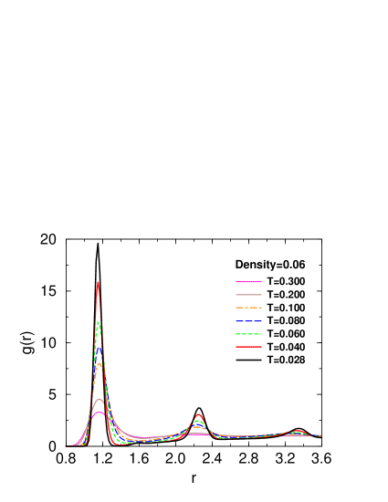
Figure 1 shows the radial distribution function, $g(r)$, for different temperatures at density $0.06$. At higher temperatures $g(r)$ shows a single peak corresponding to the interparticle distance. Additional small peaks appear at lower temperatures corresponding to second and third nearest neighbor distances, similar to dense liquids. However, here the $g(r)$ curves are characterized by relatively sharp peaks, with the gaps in between having values of $g(r)$ close to the ideal gas value of $1$ (except for low temperatures, between the first and second peaks of the $g(r)$). These features arise from the fact that the system is composed, at low temperatures, of long interconnected chains.

Figure 1: The radial distribution function, $g(r)$, at density $\rho=0.06$ for different temperatures. At high temperatures, $g(r)$ does not show much structure beyond the first peak. At low temperatures $g(r)$ exhibits multiple peaks corresponding to well defined separation distances for second, third, … nearest neighbors.

In order to study the structure on large length scales, it is useful to consider the structure factor, $S(k)$, defined as

$$S({\bf k})=\frac{1}{N}\sum_{j=1}^{N}\sum_{l=1}^{N}\left<\exp(-\mathrm{i}{\bf k}\cdot({\bf r}_{j}-{\bf r}_{l}))\right>\quad,$$ (7)

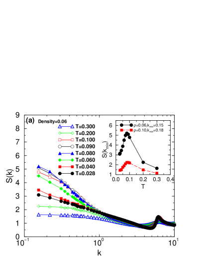
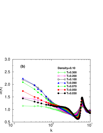
where $N$ is the total number of particles and k is the wave-vector. Figure 2 shows the $S(k)$ for a range of temperatures at density $0.06$ and $0.10$.

At high temperatures, $S(k\rightarrow 0)$ has a value close to the ideal gas value of $1$, but as the temperature is lowered, the $S(k)$ at small $k$ values gets substantially larger KobEuro . Note that at intermediate and small wave vectors, $S(k)$ shows a non-monotonic dependence on temperature, displaying a maximum value at intermediate temperatures (see inset in Fig. 2a where we show the $T$ dependence of $S(k_{min})$, i.e. the value of $S(k)$ at the smallest wave-vector $k_{min}$ that is compatible with the size of the simulation box). For $\rho=0.06$, the peak occurs at $T=0.08$, i.e. well below the percolation transition at $T=0.115$ EPAPS , where one may naively have expected the maximum to lie. The reason for the shift away from the percolation point may be rationalized by noting that in addition to percolation, which would give rise to a power-law in $S(k)$, the structure of the system changes significantly because of the formation of increasingly longer and stiffer linear chains. The latter effect will, via the form factor of the chains, also give rise to an increase in $S(k)$ at low $k$. The net effect is a shift of the temperature at which $S(k)$ has the maximum value at low wave vectors (see phase-diagram in Ref.EPAPS ). We have calculated $S(k)$ for system sizes $N=512,4000$, and $8000$ for some state points in order to investigate finite size effects and do not find any significant size effects in the form of $S(k)$.

Figure 2: The structure factor for different temperatures at (a) $\rho=0.06$ and (b) $\rho=0.10$. The $S(k)$ at the lowest wave-vector $k$ shows non-monotonic behavior in $T$ for both densities, as shown in the inset of panel (a). Temperatures below the maximum of $S(k_{min})$ are shown in solid symbols while those above are shown in open symbols to clearly indicate the non-monotonic behavior of $S(k)$.

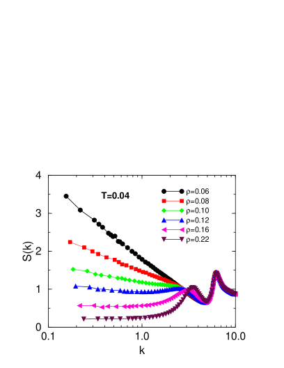
The density dependence of $S(k)$ at $T=0.04$ is shown in Fig. 3. At low densities, $\rho<0.12$, the first peak is at $k=6.15$ corresponding to the nearest neighbor distance. With an increase of the density, a peak around $k=3.0$ develops, becoming pronounced at the highest density shown; the value of $S(k)$ at the smallest wave-vectors gets suppressed, indicating a reduction in the compressibility and density fluctuations on long wavelengths.

Figure 3: The density dependence of $S(k)$ for $T=0.04$. For densities above 0.1, the large values of $S(k)$ at low $k$ get suppressed, and a finite $k$ peak develops around $k=3.0$.

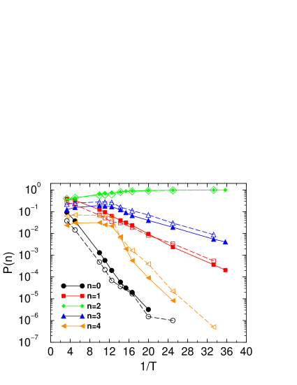
The local geometry of the system can be characterized by the distribution of the coordination number $n$. Two particles are considered to be neighbors if their distance is less than the ($T$ and $\rho$-dependent) location of the first minimum of $g(r)$. Figure 4 shows the temperature dependence of $P(n)$, the fraction of particles having coordination number $n$, vs. $1/T$ for density $\rho=0.06$ (filled symbols) and $\rho=0.10$ (open symbols). For $n=0$ and 1, the $P(n)$ decreases rapidly and monotonically as $T$ decreases, whereas for $n=2$ the $P(n)$ increases monotonically with decreasing $T$. These changes correspond to the formation of a network of particles at the expense of isolated particles or dimers. Interestingly for $n=3$ and 4 the $T-$dependence of $P(n)$ is non-monotonic, displaying a maximum at the temperature at which $S(k_{min})$ displays a maximum (see Fig. 2). Above this temperature of maximum $P(3)$ and $P(4)$, the structural change upon lowering $T$ arises from a growth in the number of bonds leading to percolation. In contrast, at temperatures below the location of the maximum, the system forms increasingly longer linear chains at the expense of cross-links with larger coordination. In contrast, in the case of the gel-forming model in KobEuro , P(3) increases with lowering of T and saturates at very low temperatures. The fraction of three-fold coordinated particles, $P(3)$, increases strongly with density (data not shown). Thus at higher density there are more anchor particles and consequently the lengths of the linear chain segments are smaller compared to that at low density.

Figure 4: The $T$-dependence of $P(n)$, the fraction of particles having coordination number $n$, at density $0.06$ (solid symbols) and $0.10$ (open symbols). At low temperatures most of the particles have coordination $n=2$. With the decrease of temperature all coordinations decrease except the one for $n=2$.

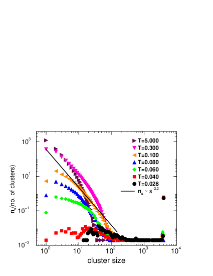
We have also calculated the cluster size distribution for density $0.06$ EPAPS . Even for temperatures near the percolation transition, we do not find a distinguishable power-law regime in the cluster size distribution, in contrast to the findings for other gel forming systems for which a power-law dependence corresponding to random percolation has been observed KobEuro ; Sciortino-ns ; Coniglio-ns . We believe this to arise from the fact that while the (exponential) cluster size distribution is obtained from a random aggregation process at high temperatures, the percolation transition is influenced by the emergence of increasingly long linear chains.

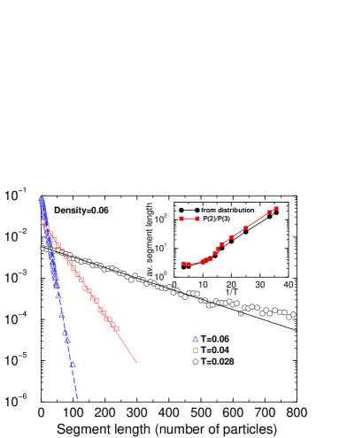
The distribution of segment lengths shows an exponential behavior (see Fig. 5), with an average segment length that increases with decreasing temperature, as can also be inferred from the $T$-dependence of $P(2)$ and $P(3)$ in Fig. 4. In the inset of Fig. 5 we show the average segment length obtained from an exponential fit to the distribution of segment lengths, as well as the ratio $P(2)/P(3)$, which provides an estimate of the average segment length. These two are in good agreement. For other densities also, the segment length distribution exhibits exponential behavior and the average segment length decreases with an increase of density.

The squared end-to-end displacement $\langle\delta^{2}(N_{c})\rangle$ of chain segments shows a quadratic behavior for small chain lengths $N_{c}$ and is linear for large $N_{c}$ shibu-thesis . The persistence length can be defined as the maximum length of a chain for which $\langle\delta^{2}(N_{c})\rangle\sim N_{c}^{2}$ holds. At $T=0.028$ and density $0.06$, the persistence length is 15 and it decreases with increasing temperature or density.

Figure 5: The segment length distribution at density $0.06$ for different temperatures, which exhibit exponential behavior. The lines are exponential fits to the data. Inset: The average segment length vs. $1/T$ from exponential fits in the main panel, and the estimate using the ratio of number of two and three coordinated particles, $P(2)/P(3)$.

IV Dynamics

In order to study the dynamics of the system we first consider the mean squared displacement (MSD) of particles, defined as

$$\langle r^{2}(t)\rangle\equiv\frac{1}{N}\sum_{i=1}^{N}\langle\Big{|}{\bf r}_{i}(t)-{\bf r}_{i}(0)\Big{|}^{2}\rangle,$$ (8)

which is shown in Fig. 6 for different $T$ at density $0.06$.

Figure 6: Mean squared displacements for different temperatures at $\rho=0.06$ in a log-log plot. The location of the $1^{st}$ and $2^{nd}$ shoulders, seen for low $T$ and discussed in the text, are marked. The bold dashed line shows the MSD from constrained simulations at $T=0.04$ (see text) which saturates at the second shoulder. The inset shows the MSD at the lowest $T$ for different densities.

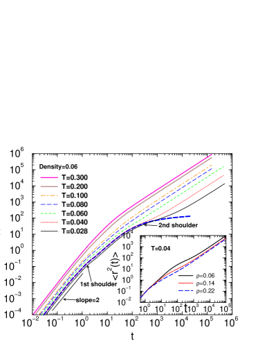
At high temperatures, a smooth crossover is seen between the short time ballistic and long time diffusive regimes. If the temperature is lowered, one sees the emergence of incipient plateaus, as seen in dense supercooled liquids. However, unlike dense liquids, one observes the presence of two “shoulders”, rather than one KobPRL . The first appears at a length of $\sim 0.4\sigma$, analogous to what is seen in dense liquids. The second shoulder appears at $\sim 7\sigma$, indicating that transient localization occurs here at a much larger length scale compared to dense liquids. Although large, this length is significantly smaller than the average segment length of the chains (around $100$ at the lowest $T$; see inset of Fig. 5). Thus, we conclude that the amplitude of floppy motions contributing to the MSD at the second shoulder is much smaller than the length of the chains.

The inset in Fig. 6 shows the evolution of the MSD at $T=0.04$ with density. As density increases, the displacement corresponding to the second shoulder decreases and also it becomes less pronounced since the segment length between anchor particles decreases.

Also included in the main panel of Fig. 6 is the MSD as obtained from constrained MD simulations at $T=0.04$, i.e. a dynamics in which bonds are prevented from breaking or forming footnote1 . As we see in the figure, the MSD from constrained MD simulations saturates at the second shoulder, indicating that the caging associated with the second shoulder is that of chain segments executing floppy motion between two anchor particles, whose magnitude is constrained by the network topology.

The non-Gaussian parameter has been studied extensively kobhet in the context of supercooled liquids as a way of characterizing dynamical heterogeneities. The non-Gaussian parameter $\alpha_{2}(t)$ is defined asBoon ; odagaki_hiwatari_91

$$\alpha_{2}(t)\equiv\frac{3\langle r^{4}(t)\rangle}{5\langle r^{2}(t)\rangle^{2}}-1\quad,$$ (9)

where

$$\langle r^{4}(t)\rangle\equiv\frac{1}{N}\langle\sum_{i=1}^{N}\Big{|}{\bf r}_{i}(t)-{\bf r}_{i}(0)\Big{|}^{4}\rangle\quad.$$ (10)

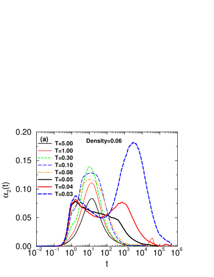
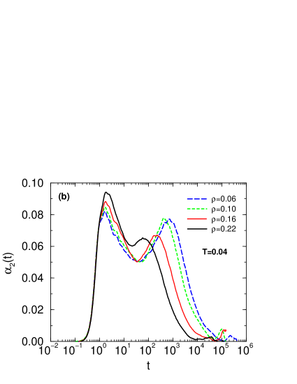
Figure 7a shows $\alpha_{2}(t)$ for different $T$ at density $0.06$. At high temperatures, a single peak in $\alpha_{2}(t)$ is observed at around $t=10$, a time that corresponds to the crossover in the MSD from ballistic to diffusive behavior. At intermediate temperatures, an additional peak at $t\approx 1$ emerges, which is the time at which the first shoulder in the MSD is observed. Its origin is likely the heterogeneous dynamics related to the fact that different particles can have quite different type of cages since they can be two or three-fold coordinated. If $T$ is decreased even further, the location of the peak at longer times rapidly shifts to larger times, and its height increases with decreasing $T$. This peak corresponds to the second shoulder seen in the MSD. We note that the height of this peak is, even at the lowest temperatures, less than 0.2, a value that is significantly smaller than the ones that are found in dense glass-forming systems, such as, e.g. Lennard-Jones mixtures kob_andersen_95a for which $\alpha_{2}(t_{max})\approx 1.5$. This difference is probably due to the fact that in the present system there is, at low temperatures, not that much variance in the relaxation dynamics of the individual particles since the main relaxation process is a cutting of a chain and a subsequent reconnection of the loose ends to the rest of the network. This process depends only very weakly on the particle considered and hence the $\alpha_{2}(t)$ is small.

In Fig. 7b we show the density dependence of the non-Gaussian parameter for $T=0.04$. The position of the first peak, around $t=1$, is independent of density whereas the second peak position moves to larger times with decreasing density, in agreement with the density dependence of the MSD on the time scale of the second shoulder.

Figure 7: The non-Gaussian parameter $\alpha_{2}(t)$ for (a) different $T$ at density $0.06$ and (b) different densities at $T=0.04$.

To study the life time of the bonds, we calculate the bond correlation function $\phi_{B}(t)$ defined asSciortino ; Starr1 ; Starr2

$$\phi_{B}(t)=\frac{\left<\sum_{i<j}\delta n_{ij}(t)\delta n_{ij}(0)\right>}{\left<\sum_{i<j}\delta n_{ij}(0)\delta n_{ij}(0)\right>}\quad,$$ (11)

where

$$\delta n_{ij}(t) = n_{ij}(t)-\langle n\rangle$$

$$\mbox{and }n_{ij} = 1-H(r_{ij}-r_{cut})\quad.$$ (12)

$H(x)$ is the Heaviside function and $r_{cut}$ is the bond length defined as the distance at which the first minimum of $g(r)$ occurs. $n_{ij}$ is $1$ when a bond is present and $0$ otherwise. Hence, $\phi_{B}(t)$ counts the fraction of bonds found at $t=0$ that survive after a time $t$, independent of any breaking and reforming at intervening times. Figure 8 shows the bond correlation function at density $0.06$ for different temperatures (upper curves) and at $T=0.04$ for different densities (lower curves). (For the sake of clarity, the lower curves have been shifted down by a factor of $100$.) In order to recognize better the $T$ and $\rho-$dependence of this correlation function we plot it as a function of $t/\tau_{B}$, where $\tau_{B}$ is the average bond life time as determined from the area under $\phi_{B}(t)$. We see that the bond correlation functions decay exponentially with time at low $T$, but that the decay is slower than exponential at intermediate temperatures. At high $T$ the decay is again exponential (data not shown). Similarly, at $T=0.04$, the decay behavior is exponential at low densities and stretched exponential at higher densities. In both cases, the stretched exponential behavior appears to be associated with an increase of disorder in the local environment of the bonds.

Figure 8: The bond correlation function $\phi_{B}(t)$ as a function of $t/\tau_{B}$ at different temperatures and density $0.06$ (upper curves ) and at different densities for $T=0.04$ (lower curves). The latter set of curves has been shifted down by a factor of $100$ for the sake of clarity. $\tau_{B}$ is the average bond life time.

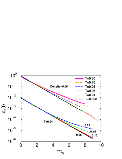
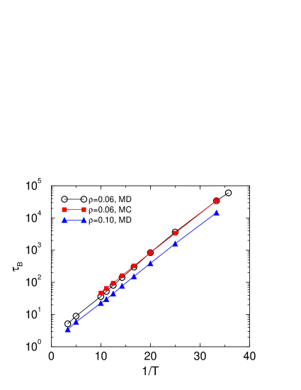
Figure 9 shows the $T$-dependence of the bond life time, $\tau_{B}$, for density $0.06$ and $0.10$ from MD simulations as well as the $\tau_{B}$ from MC simulations at density $0.06$. We recognize from the figure that the bond life times from MD and MC simulations compare well with each other after scaling the MC times (expressed in number of sweeps) by a single multiplicative factor of 100. This shows that the relaxation dynamics does not depend on the details of the microscopic dynamics. $\phi_{B}(t)$ exhibits an Arrhenius behavior with an activation energy of $0.28$.

Figure 9: The bond lifetime $\tau_{B}$ vs. inverse $T$ at density $0.06$ and $0.10$ from MD simulations and from MC simulations for density $0.06$.

One of the most useful quantities for the study of dynamics is the intermediate scattering function $F(k,t)$ defined as Hansen-McDonald

$$F(k,t)=\frac{1}{N}\sum_{l=1}^{N}\sum_{j=1}^{N}\langle\exp[-\mathrm{i}{\bf k}\cdot({\bf r}_{l}(t)-{\bf r}_{j}(0))]\rangle.$$ (13)

$F(k,t)$ provides information on the collective dynamics of the system. The self intermediate scattering function, $F_{s}(k,t)$, which reveals information about single particle motion, is obtained by restricting the double summation above to $l=j$:

$$F_{s}(k,t)=\frac{1}{N}\sum_{j=1}^{N}\langle\exp[-\mathrm{i}{\bf k}\cdot({\bf r}_{j}(t)-{\bf r}_{j}(0))]\rangle.$$ (14)

Figure 10 shows $F(k,t)$ vs. time $t$ for different wave-vectors $k$ at $T=0.04$ and density $\rho=0.06$. From this graph we recognize that $F(k,t)$ shows three regimes: At very short times the function is quadratic in $t$, since we have a Newtonian dynamics. At long times the function shows at small $k$ an oscillatory behavior which is related to the usual acoustic sound modes. The most remarkable feature is seen at intermediate times where we find that $F(k,t)$ shows a compressed exponential decay, $F(k,t)=\exp(-(t/\tau)^{\beta})$, with an exponent $\beta\approx 3/2$ for all $k$-values shown. (For $k$ values that are even larger than the ones shown in Fig. 10, one finds that $F(k,t)$ decays ballistically, i.e. $\beta\approx 2$, see Ref. shibuPRL .) Also included in the graph are fits with a Kohlrausch-Williams-Watts (KWW) function with an exponent of $3/2$. Such compressed exponential relaxation, i.e. $\beta>1$, has been observed in experiments on non-equilibrium colloidal gels and it has been argued that this compression is related to the stress inhomogeneities caused by the shrinking of the gelsCipelletti ; pitard . In the present case, the system is in equilibrium and the compressed exponential behavior is due to the floppy motion of the non-restructuring network present in the gel-formershibuPRL , as we will show below.

It is also of interest to note that even at this low temperature there is no sign of the two-step relaxation observed in dense glass-forming liquids (see, e.g., Ref. kob_andersen_95b ). Thus we have here an example of a system whose relaxation dynamics is glassy (non-exponential, strong $T-$dependence, complex $k-$dependence,…) but with correlation functions that do not show the caging regime at intermediate times (at least in the $k$ and $T-$range accessible in this simulation).

In order to get a better understanding of the origin of the compressed exponential it is useful to compare the time dependence of $F(k,t)$ with the one of the bond correlation function $\phi_{B}(t)$. This is done in Fig. 11, where we show $F(k,t)$ for the smallest wave-vector as well as the bond correlation function for $T=0.04$, $\rho=0.06$. Also included is the bond correlation function defined only for particles that initially have three-fold coordination. It is seen that $F(k,t)$ decays with a compressed exponential form on a time scale that is much shorter than the bond life time for all particles, and also in which a substantial fraction of bonds associated with initially three-coordinated particles are still intact. This observation suggests that the compressed exponential relaxation seen is due to the dynamics of the gel network on time scales when bond breaking is not very relevant.

To confirm this, we have performed constrained MD simulations, i.e. a dynamics in which bonds are prevented from breaking or forming footnote1 . Figure 12 shows $F(k,t)$ with and without the presence of this constraint potential. The two $F(k,t)$ curves are essentially identical in the time regime where compressed exponential relaxation is seen, but deviate from each other at later times, with the constrained MD curve saturating to a finite value. The data shown in Fig. 12 clearly demonstrates that the origin of the compressed exponential relaxation is in the vibrational dynamics of the gel network.

Figure 10: The collective intermediate scattering function $F(k,t)$ at $\rho=0.06$ and $T=0.04$ for different wave-vectors $k$. The KWW fit to $F(k,t)$ at intermediate times with an exponent $\beta=3/2$ is also included (dashed lines).

Figure 11: The collective intermediate scattering function $F(k,t)$ and the bond correlation function $\phi_{B}(t)$ at density $0.06$ and $T=0.04$. Also shown is the bond correlation function for particles which are initially three-fold coordinated.

Figure 12: The collective intermediate scattering function $F(k,t)$ for different wave-vectors $k$ at density $\rho=0.06$ and $T=0.04$ from MD (solid lines) and constrained MD simulation (dashed lines).

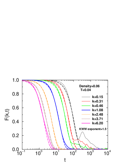
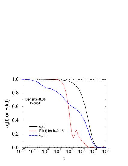
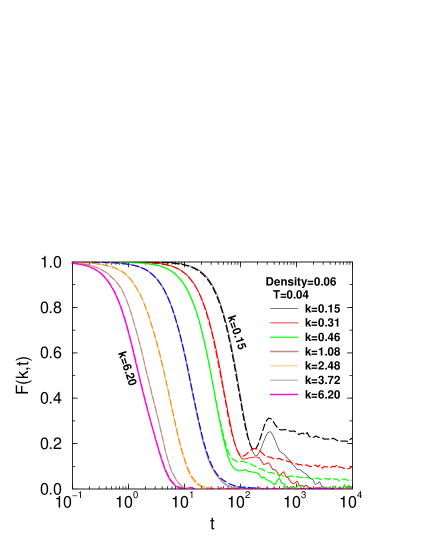
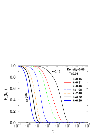
Figure 13 shows the time dependence of the self intermediate scattering function $F_{s}(k,t)$ at density $0.06$ and temperature $T=0.04$ for different wave-vectors. At long times, the decay is close to exponential for small wave vectors and faster than exponential at large wave vectors shibuPRL . A close inspection of Fig. 13 reveals that the stretching exponent varies non-monotonically, and is smaller at intermediate wave vectors. This behavior holds at other low temperatures as well shibuPRL . A comparison with the behavior of $F(k,t)$ shows that these two functions indeed reveal very different aspects of the dynamics of the gel former.

Figure 13: The self intermediate scattering function $F_{s}(k,t)$ from MD simulations for $\rho=0.06$ and $T=0.04$ for different wave-vectors $k$.

Figure 14: The $k-$dependence of $\tau_{s}$ multiplied by $k^{2}$, where $\tau_{s}$ has been obtained from the area of $F_{s}(k,t)$, at different $T$ at $\rho=0.22$ (filled symbols) and $\rho=0.06$ (open symbols).

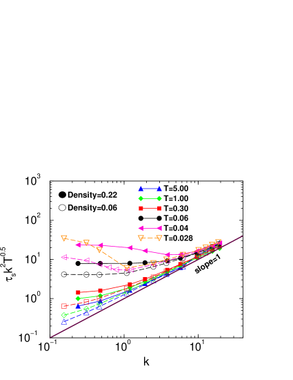
In Fig. 14 we show the relaxation time $\tau_{s}$ that have been calculated from the area under $F_{s}(k,t)$ vs. time for different wave vectors at densities $0.06$ (open symbols) and $0.22$ (filled symbols). (In order to compensate the trivial $1/T^{0.5}$ dependence at large $k$, we multiply the data by $T^{0.5}$.) At high wave-vectors the linear behavior of $\tau_{s}k^{2}$ indicates the ballistic character of the dynamics, consistent with the gaussian behavior of $F_{s}(k,t)$ shown in Fig. 13 and the value for the KWW exponent which is around 2.0 (see Ref. shibuPRL ). For intermediate temperatures, we observe a crossover to a regime where $\tau_{s}k^{2}$ is roughly constant at small wave vectors, seemingly indicating a diffusive dynamics. However, the $F_{s}(k,t)$ curves shown in Fig. 13 reveal that the dynamics is more complex than a simple diffusive behavior in these cases. Note that the location in $k$ at which this crossover is observed depends strongly on temperature and density, which indicates the complex dependence of the relaxation dynamics on $\rho$ and $T$. This conclusion is also supported by the observation that at the lowest temperature investigated the mentioned plateau at low $k$ disappears (see Fig. 14) since the stiffening of the network pushes the hydrodynamic regime to even lower values of $k$, in agreement with previous results KobPRL .

The relaxation times ($\tau$ and $\tau_{s}$) and $\tau_{B}$ at $T=0.04$ and wave-vector $k=2\pi\times 2/L$, i.e.  the second smallest wave-vector compatible with the size $L$ of the simulation box, is shown in Fig. 15. The relaxation times $\tau_{s}$, $\tau$ have been obtained from the area under $F_{s}(k,t)$, $F(k,t)$ vs. time curves. We recognize that $\tau_{B}$ as well as $\tau$ decrease with increasing density. The reason for this is that with increasing $\rho$ the number of short lived three and higher coordinated particles increases, with the consequences that: (i) $\tau_{B}$ of the system decreases and (ii) the network structure can reconstruct more easily, in turn leading to a faster decay of $F(k,t)$, and a decrease of $\tau$.

On the other hand, $\tau_{s}$ is nearly independent of density. This is a consequence of the fact that the MSD is roughly the same for all densities in the diffusive regime (see Fig. 6). However, at larger wave-vectors, $\tau_{s}$ shows a more significant dependence on density (data not shown) shibu-thesis , consistent with significant changes in the MSD near the second shoulder.

Figure 15: The density dependence of the bond life time $\tau_{B}$ and relaxation times $\tau$ and $\tau_{s}$ obtained from the area of the coherent and incoherent intermediate scattering functions for $T=0.04$ and wave-vector $k={2\pi\over L}\times 2L$, where $L$ is the size of the simulation box.

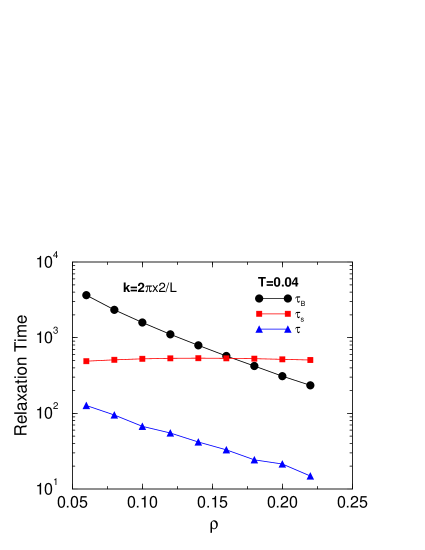
Since in real experiments the relaxation dynamics of the gels is given by a Brownian dynamics instead of the Newtonian dynamics studied here, it is of interest to investigate which properties of the relaxation dynamics depend on the microscopic dynamics. In the final part of this paper we therefore compare $F(k,t)$ and $F_{s}(k,t)$ obtained from MD with those obtained from MC.

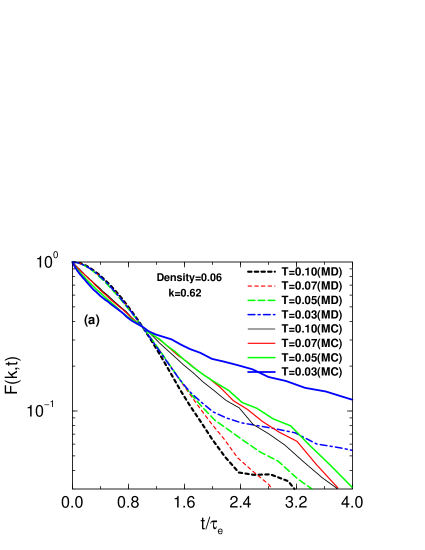
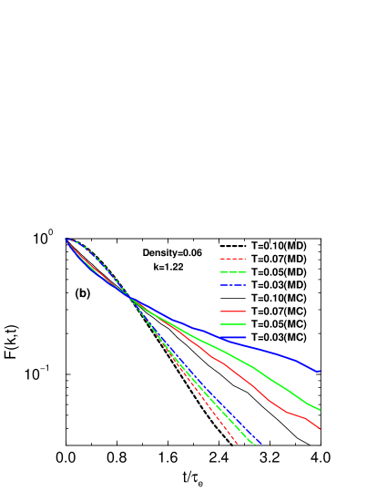
In Fig. 16 we show the coherent intermediate scattering function $F(k,t)$ vs. time for different $T$’s and $k=0.31$ obtained from MC as well as MD simulations. In order to allow to show the curves for different temperatures on the same graph, we plot the correlators as a function of $t/t_{\rm e}$, where $t_{\rm e}$ is the time at which the $F(k,t)$ reaches a value of $1/e$. From the graph we see that the relaxation behavior of $F(k,t)$ from the MC and MD simulations are quite different: Independent of $k$ EPAPS , the $F(k,t)$ from MC shows an exponential relaxation at the highest temperature shown ($T=0.10$), and becomes progressively more stretched as temperature decreases. On the other hand, MD simulations exhibit compressed exponential for all $T$, although a slower decay is apparent at lower $T$ due to the presence of acoustic modes. Thus we conclude that the MC dynamics suppresses the intermediate time compressed exponential behavior and allows one to see the stretched exponential decay at long times (see also Ref. shibuPRL ).

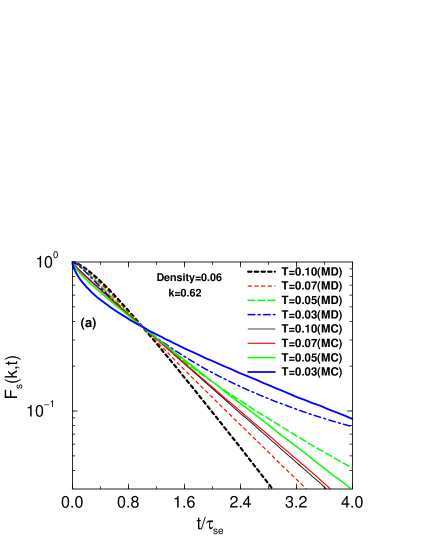
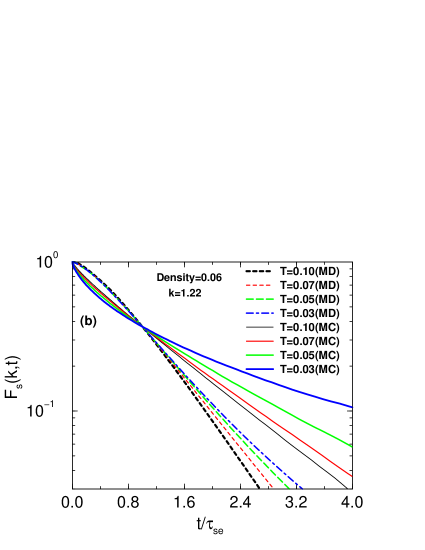
Last but not least we show in Fig. 17 the incoherent intermediate scattering function $F_{s}(k,t)$ vs. $t/t_{\rm se}$ for different $T$ and $k$ obtained from MC as well as MD simulations. The $F_{s}(k,t)$ curves from MC are nearly exponential at the lower $k$ values and higher $T$, showing stretching at the lowest $T$ for all $k$ values, and for all $T$ at $k=1.22$ EPAPS . The degree of stretching increases with decrease of $T$ and an increase of $k$. In contrast to this, $F_{s}(k,t)$ from MD shows a compressed exponential behavior for all $T$ at $k=1.22$ EPAPS , but at smaller $k$ the behavior becomes stretched at the two lowest temperatures.

Figure 16: The collective intermediate scattering function $F(k,t)$ vs. time, for density = $0.06$, in log-linear scale as obtained from MD (dashed lines) and MC (solid lines) for $k=0.31$.

Figure 17: The self intermediate scattering function $F_{s}(k,t)$ vs. time, for density = $0.06$, in log-linear scale as obtained from MD (dashed lines) and MC (solid lines) for $k=0.31$.

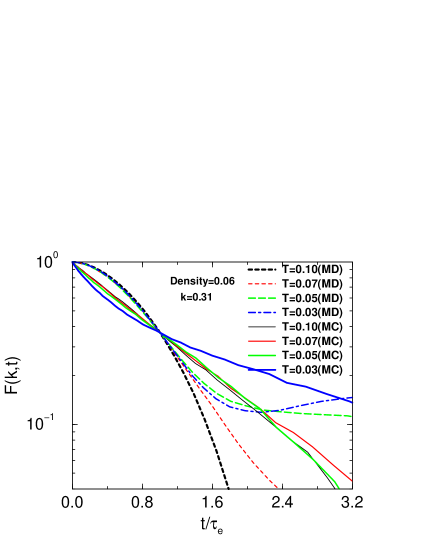
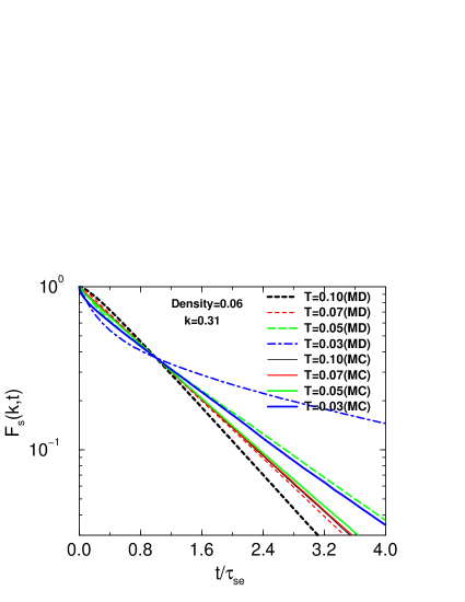
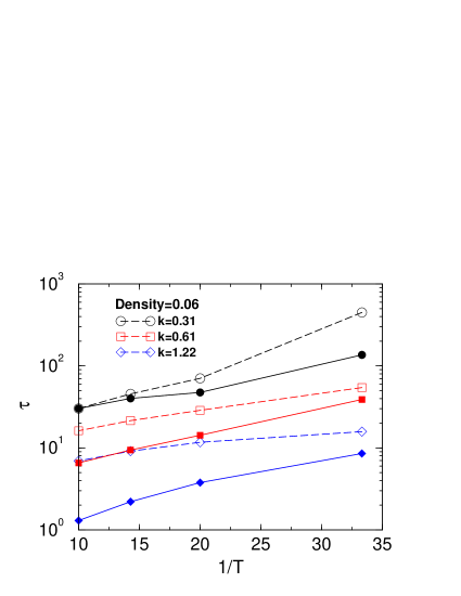
Figure 18 shows the $T-$dependence of $\tau$ obtained from the area under $F(k,t)$ from MD and MC simulations for wave-vector $k=0.31$, $0.61$ and $1.22$ at density $0.06$. The data in Fig. 18 have been plotted by rescaling the MC relaxation times to be the same at $k=0.31$ for the highest $T$. We see that at $T=0.1$ the $k-$dependence of $\tau$ is much stronger for the MD than for the MC. Furthermore we recognize that the $T-$dependence of $\tau$ is stronger in the case of the MD than for the MC. Thus, the long time behavior as revealed by MC is substantially different from the self and collective intermediate scattering functions obtained from MD. This result also implies that from the point of view of simulations it is more efficient to equilibrate the system using MC.

Figure 18: The $T-$dependence of the relaxation times obtained from the area under the coherent intermediate scattering function in MC (filled symbols) and MD (open symbols) simulations at density $\rho=0.06$ for different wave-vectors. The MC data are scaled by a factor $2000$ chosen such that the MC relaxation time at $k=0.31$ coincides with the corresponding MD time at the highest temperature.

V Summary and conclusions

In this paper we have investigated the static and dynamic properties of a recently introduced model for gel-forming systems. The gel-forming ability of this model is related to the fact that its local three-body potential avoids the formation of dense local structures and instead favors an open network structure. Due to this feature, the liquid-gas phase separation is pushed to low densities and temperatures, thus opening at intermediate densities a temperature range in which the relaxation dynamics is very slow, i.e. the system is a gel in equilibrium. Although this mechanism for the formation of the gel is similar to the approaches proposed earlier delgado ; fsrev ; Blaak , the simplicity of the chosen interaction potential makes the present model very attractive for simulations. This advantage is enhanced even further by the use of an efficient method, presented in the Appendix, to evaluate the mentioned three-body potential. Making use of this computational gain we have been able to characterize in detail the properties of the system, in equilibrium, in a significant range of temperature and density.

We find that with decreasing temperature the particles assemble in the form of long one-dimensional chains that are connected to each other at random points, i.e. the system does indeed form a very heterogeneous network in which the length of the bridging chains follows an exponential distribution. The static structure factor of this spanning open network shows a strong increase at small wave-vectors for temperatures that are close to, but not quite at, the percolation line. The reason for this shift, which depends on density, is the fact that at large scales $S(k)$ is not only given by the open structure of the percolating network but that there are also contributions from the form-factor of the chains.

The bond correlation function $\phi_{B}(t)$ shows at moderately low temperatures and high densities a non-exponential time dependence, which is related to the complex relaxation dynamics on the length scale of two particles, in analogy to the relaxation dynamics of dense glass-forming liquids. In contrast to this, $\phi_{B}(t)$ shows at very low temperatures and densities an exponential $t-$dependence, indicating a very simple bond breaking mechanism with an activation energy that is only a very weak function of $T$. We note that this result is independent of the used microscopic dynamics (molecular dynamics or Monte Carlo), which shows that this dynamical property is closely related to the structure of the system, as it has been found in other glass-forming systems gleim ; berthier ; berthier_kob_07 .

In contrast to this, the time correlation functions $F(k,t)$ and $F_{s}(k,t)$ show a significant dependence on the microscopic dynamics. For $F(k,t)$ as obtained from the MD we find a compressed exponential for length scales that are smaller or comparable to the one of the size of the particles, and acoustic modes for larger scales. On the other hand, the MC dynamics shows stretched exponentials for all length scales. The same trend is seen for $F_{s}(k,t)$, except that there are (of course) no acoustic modes in the MD. Thus we conclude that a dissipative dynamics, relevant for the experimental systems, does not show the compressed exponential relaxation observed in experiments in which the sample was aging. In experiments, therefore, the out-of-equilibrium nature of the samples must play an important role for the compressed exponential relaxation. Investigating the details of how the out-of-equilibrium dynamics leads to the experimentally observed compressed exponential relaxation remains an open problem that should be investigated in the future.

Appendix: Efficient method for force calculation of the SW potential

Here we describe an efficient method for the calculation of energy and forces for the Stillinger-Weber potential, which involves only double sums to calculate three-body interaction energies and forces. We follow the approach by Makhov and LewisMakhov-Lewis for energy calculations (see also Frenkel-2loop ; W-S1993 ) but extend it to the calculation of forces.

V.1 Energy Calculation

From Eqs. (1)-(6) it follows that the Stillinger-Weber potential can be written as

$$u_{SW}=\sum_{i}\sum_{j>i}{v}_{2}(r_{ij})+\sum_{i}\sum_{j\neq i}\sum_{k\neq i,j}\frac{1}{2}\phi({\bf r}_{ij},{\bf r}_{ik})\quad$$ (15)

with distances expressed in units of $\sigma$ and $\phi$ denotes

$$\phi({\bf r}_{ij},{\bf r}_{ik}) = \epsilon\lambda\exp\Big{(}\frac{\gamma}{r_{ij}-a}+\frac{\gamma}{r_{ik}-a}\Big{)}(\cos\theta_{jik}+\alpha)^{2}$$ (16)

$$\times H(a-r_{ij})H(a-r_{ik})$$

We define $\tilde{\lambda}=\epsilon\lambda$, and the quantities

$$g_{ij} = \left\{\begin{array}[]{ll}\exp\left[\frac{\gamma}{r_{ij}-a}\right]&r_{ij}<a\\ 0&r_{ij}\geq a\end{array}\right.,$$ (19)

and

$$U_{i}^{d} = \tilde{\lambda}\sum_{j\neq i,k\neq i}\frac{1}{2}g_{ij}\mbox{ }g_{ik}(\cos\theta_{jik}+\alpha)^{2}$$ (21)

$$= \tilde{\lambda}\sum_{j\neq i,k\neq i}\Big{[}\frac{1}{2}g_{ij}\mbox{ }g_{ik}\alpha^{2}+\alpha g_{ij}\mbox{ }g_{ik}\mbox{ }\cos\theta_{jik}$$

$$+\frac{1}{2}g_{ij}\mbox{ }g_{ik}\mbox{ }\cos^{2}\theta_{jik}\Big{]}\quad.\qquad\qquad\qquad\qquad\quad$$

With these definitions the three-body potential term in Eq. (15) can be written as a sum over $U_{i}^{d}$,

$$\sum_{r_{ij},r_{ik}<a}\frac{1}{2}\phi({\bf r}_{ij},{\bf r}_{ik})=\sum_{i}(U_{i}^{d}-{U_{ij}^{c}}^{\prime})\quad,$$ (22)

where the correction ${U_{ij}^{c}}^{\prime}$ is due to the fact that $U_{i}^{d}$ contains the terms $j=k$, see Eq. (21), whereas the sum on the left hand side of Eq. (22) does not include them.

One easily finds that

$${U_{ij}^{c}}^{\prime}=\sum_{j\neq i}\frac{1}{2}\tilde{\lambda}g_{ij}^{2}\mbox{ }(1+\alpha)^{2}\quad,$$ (23)

i.e.  this is a two-body term.

Defining thus

$$v_{ij}^{eff}=v_{2}(r_{ij})-U_{ij}^{c}\quad,$$ (24)

where $U_{ij}^{c}=2{U_{ij}^{c}}^{\prime}$, the total potential energy becomes

$$u_{SW}=\sum_{i}\sum_{j>i}v_{ij}^{eff}+\sum_{i}U_{i}^{d}.$$ (25)

The factor $1/2$ in Eq. (23) is to account for the double counting of pair distances, which is not present in the first term of Eq. (25) and is, therefore, omitted. In the following we will show that the term $U_{i}^{d}$ can be evaluated by a single loop over the neighbors of particle $i$, thus allowing us to evaluate the energy of the system without evaluating a triple sum. For this we define the quantity $h_{i}$ as

$$h_{i}=\sum_{j\neq i}g_{ij},$$ (26)

and find

$$h_{i}^{2}=\left|\sum_{j\neq i}g_{ij}\right|^{2}=\sum_{j,k\neq i}g_{ij}\mbox{ }g_{ik}\quad.$$ (27)

which is proportional to the first term on the right hand side of Eq. (21).

Similarly we define

$${\bf s}_{i}=\sum_{j\neq i}g_{ij}\hat{\bf r}_{ij}$$ (28)

where $\hat{\bf r}_{ij}={\bf r}_{ij}/r_{ij}$ to obtain

$$|{\bf s}_{i}|^{2} = \left|\sum_{j\neq i}g_{ij}\mbox{ }\hat{\bf r}_{ij}\right|^{2}=\sum_{j,k\neq i}g_{ij}\mbox{ }g_{ik}(\hat{\bf r}_{ij}.\hat{\bf r}_{ik})$$ (29)

$$= \sum_{j,k\neq i}g_{ij}\mbox{ }g_{ik}\mbox{ }\cos\theta_{jik}.$$ (30)

Finally, we define ${\bf T}_{i}$

$${\bf T}_{i}=\sum_{j\neq i}g_{ij}(\hat{\bf r}_{ij}\otimes\hat{\bf r}_{ij})\quad,$$ (31)

where $\otimes$ denotes the outer product, and obtain

$$Tr[{{\bf T}_{i}}^{2}] = \sum_{j,k\neq i}Tr[g_{ij}(\hat{\bf r}_{ij}\otimes\hat{\bf r}_{ij})g_{ik}(\hat{\bf r}_{ik}\otimes\hat{\bf r}_{ik})]$$

$$= \sum_{j,k\neq i}g_{ij}g_{ik}(\hat{\bf r}_{ij}.\hat{\bf r}_{ik})^{2}$$

$$= \sum_{j,k\neq i}g_{ij}g_{ik}\cos^{2}\theta_{jik}.$$ (33)

Thus we find that $U_{i}^{d}$ is a sum of three terms, each of which involves only a single sum over the neighbors of particle $i$:

$$U_{i}^{d}=\frac{\tilde{\lambda}}{2}\alpha^{2}h_{i}^{2}+\tilde{\lambda}\alpha|{\bf s}_{i}^{2}|+\frac{\tilde{\lambda}}{2}Tr[{\bf T}_{i}^{2}]$$ (34)

This expression thus allows us to calculate efficiently the total potential energy of the system using a double sum.

V.2 Force Calculation

The force acting on the $i^{th}$ particle is given by

$${\bf F}_{i} = -\nabla_{i}u_{SW}$$ (35)

$$= -\Big{[}\sum_{j\neq i}\frac{\partial v_{2}(r_{ij})}{\partial r_{ij}}\hat{\bf r}_{ij}+\nabla_{i}U_{i}^{d}+\sum_{j\neq i}\nabla_{i}U_{j}^{d}$$

$$-\sum_{j\neq i}\frac{\partial U_{ij}^{c}}{\partial r_{ij}}\hat{\bf r}_{ij}\Big{]}.$$

From Newton’s third law of motion, we have

$$\nabla_{i}U_{i}^{d} = -\sum_{j\neq i}\nabla_{j}U_{i}^{d}.$$ (36)

Thus,

$${\bf F}_{i} = -\Big{[}\sum_{j\neq i}\frac{\partial v_{2}(r_{ij})}{\partial r_{ij}}\hat{\bf r}_{ij}+\sum_{j\neq i}(\nabla_{i}U_{j}^{d}-\nabla_{j}U_{i}^{d})$$

$$-\sum_{j\neq i}\frac{\partial U_{ij}^{c}}{\partial r_{ij}}\hat{\bf r}_{ij}\Big{]},$$

where derivatives of trivial two-body terms are given as,

$$\frac{\partial v_{2}(r_{ij})}{\partial r_{ij}} = -\epsilon A\Big{[}4Br_{ij}^{-5}+\frac{Br_{ij}^{-4}-1}{(r_{ij}-a)^{2}}$$ (38)

$$\times\exp\left(\frac{1}{r_{ij}-a}\right)\Big{]}$$

and

$$\frac{\partial U_{ij}^{c}}{\partial r_{ij}} = 2\tilde{\lambda}(1+\alpha)^{2}g_{ij}\frac{\partial g_{ij}}{\partial r_{ij}}.$$ (39)

The non-trivial part of the calculation is the calculation of $\nabla_{j}U_{i}^{d}$:

$$\nabla_{j}U_{i}^{d} = \frac{\tilde{\lambda}}{2}\alpha^{2}\nabla_{j}h_{i}^{2}+\tilde{\lambda}\alpha\nabla_{j}|{\bf s}_{i}^{2}|+\frac{\tilde{\lambda}}{2}\nabla_{j}Tr[{\bf T}_{i}^{2}].$$ (40)

Each of the terms are evaluated below.

• Calculation of $\nabla_{j}h_{i}^{2}$:

  $$\nabla_{j}h_{i}^{2} = 2h_{i}\nabla_{j}h_{i}$$ (41)

  $$= 2h_{i}\nabla_{j}\sum_{j\neq i}g_{ij}$$ (42)

  $$= 2h_{i}\frac{\partial g_{ij}}{\partial r_{ij}}\hat{\bf r}_{ij}$$ (43)

  $$= 2\frac{h_{i}}{{r}_{ij}}\frac{\partial g_{ij}}{\partial r_{ij}}{\bf r}_{ij}$$ (44)

• Calculation of $\nabla_{j}|{\bf s}_{i}^{2}|$:

  We have $\nabla_{j}|{\bf s}_{i}^{2}|$ = $\nabla_{j}({\bf s}_{i}.{\bf s}_{i})$. The gradient of the dot product of two vectors X and Y is given by,

  $$\nabla({\bf X}.{\bf Y})=({\bf X}.\nabla){\bf Y}+({\bf Y}.\nabla){\bf X} + {\bf X}\times(\nabla\times{\bf Y})$$ (45)

  $$+ {\bf Y}\times(\nabla\times{\bf X}).$$

  Therefore, $\nabla_{j}({\bf s}_{i}.{\bf s}_{i})=2(\nabla{\bf s}_{i})\mbox{}{\bf s}_{i}$. The gradient of vector ${\bf s}_{i}$ is a tensor of rank two i.e. a matrix and is given as,

  $$\nabla_{j}{\bf s}_{i} = \nabla_{j}(g_{ij}\hat{\bf r}_{ij})$$ (46)

  $$= \frac{\partial g_{ij}}{\partial r_{ij}}(\hat{\bf r}_{ij}\otimes\hat{\bf r}_{ij})+g_{ij}\nabla_{j}(\hat{\bf r}_{ij})$$ (47)

  $$= \frac{\partial g_{ij}}{\partial r_{ij}}(\hat{\bf r}_{ij}\otimes\hat{\bf r}_{ij})+\frac{g_{ij}}{r_{ij}}\left[{\bf I}-\hat{\bf r}_{ij}\otimes\hat{\bf r}_{ij}\right],$$ (48)

  where we have used the fact that,

  $$\nabla_{j}\hat{\bf r}_{ij}=\frac{1}{r_{ij}}({\bf I}-\hat{\bf r}_{ij}\otimes\hat{\bf r}_{ij}).$$ (49)

  Hence,

  $$\nabla_{j}{\bf s}_{i} = \frac{g_{ij}}{r_{ij}}{\bf I}+\left(\frac{\partial g_{ij}}{\partial r_{ij}}-\frac{g_{ij}}{r_{ij}}\right)(\hat{\bf r}_{ij}\otimes\hat{\bf r}_{ij}).$$ (50)

  Now, the gradient of $|{\bf s}_{i}|^{2}$ is given by,

  $$\nabla_{j}|{\bf s}_{i}|^{2} = 2(\nabla_{j}{\bf s}_{i})\mbox{ }{\bf s}_{i}$$

  $$= 2\left(\frac{\partial g_{ij}}{\partial r_{ij}}-\frac{g_{ij}}{r_{ij}}\right)(\hat{\bf r}_{ij}\otimes\hat{\bf r}_{ij})\mbox{ }{\bf s}_{i}$$

  $$+ 2\frac{g_{ij}}{r_{ij}}{\bf s}_{i}$$ (52)

  where we have used the fact that,

  $${\bf I}\mbox{ }{\bf s}_{i} = {\bf s}_{i}$$ (53)

  $$\mbox{and, }(\hat{\bf r}_{ij}\otimes\hat{\bf r}_{ij}){\bf s}_{i} = (\hat{\bf r}_{ij}.{\bf s}_{i})\hat{\bf r}_{ij}$$ (54)

  $$= \frac{1}{r_{ij}^{2}}({\bf r}_{ij}.{\bf s}_{i}){\bf r}_{ij}.$$ (55)

  Finally, the gradient of $|{\bf s}_{i}|^{2}$ is written as,

  $$\nabla_{j}|{\bf s}_{i}|^{2} = 2\left(\frac{\partial g_{ij}}{\partial r_{ij}}-\frac{g_{ij}}{r_{ij}}\right)\left(\frac{{\bf s}_{i}.{\bf r}_{ij}}{r_{ij}^{2}}{\bf r}_{ij}\right)+2\frac{g_{ij}}{r_{ij}}{\bf s}_{i}.$$ (56)

• Calculation of $\nabla_{j}Tr[{\bf T}_{i}^{2}]$:

  We use the fact that

  $$\frac{\partial x^{n}}{\partial x}=n\frac{\partial(xA^{n-1})}{\partial x}\Bigg{|}_{A=x}.$$ (57)

  Therefore, for a constant matrix A,

  $$\nabla_{j}Tr[{\bf T}_{i}^{2}] = 2\nabla_{j}Tr({\bf T}_{i}{\bf A})\Big{|}_{{\bf A}={\bf T}_{i}}$$ (58)

  $$= 2\nabla_{j}Tr[g_{ij}(\hat{\bf r}_{ij}\otimes\hat{\bf r}_{ij}{\bf A})]\Big{|}_{{\bf A}={\bf T}_{i}}$$ (59)

  One easily finds that,

  $$Tr[g_{ij}(\hat{\bf r}_{ij}\otimes\hat{\bf r}_{ij}{\bf A})]=\Big{(}\frac{g_{ij}{\bf r}_{ij}.{\bf A}{\bf r}_{ij}}{r_{ij}^{2}}\Big{)}.$$ (60)

  Therefore, the gradient of trace of $T_{i}^{2}$ matrix is given by

  $$\nabla_{j}Tr[{\bf T}_{i}^{2}] = 2\nabla_{j}\left(\frac{g_{ij}{\bf r}_{ij}.{\bf A}{\bf r}_{ij}}{r_{ij}^{2}}\right)\Big{|}_{{\bf A=T}_{i}}$$ (63)

  $$= 2\frac{\partial g_{ij}}{\partial r_{ij}}\left(\frac{{\bf r}_{ij}.{\bf T}_{i}{\bf r}_{ij}}{r_{ij}^{2}}\right)\hat{\bf r}_{ij}$$

  $$+2g_{ij}\nabla_{j}\left(\frac{{\bf r}_{ij}.{\bf A}{\bf r}_{ij}}{r_{ij}^{2}}\right)$$

  $$= 2\frac{\partial g_{ij}}{\partial r_{ij}}\left(\frac{{\bf r}_{ij}.{\bf T}_{i}{\bf r}_{ij}}{r_{ij}^{2}}\right)\hat{\bf r}_{ij}$$

  $$+2g_{ij}(-\frac{2}{r_{ij}^{3}})({\bf r}_{ij}.{\bf A}{\bf r}_{ij})\hat{\bf r}_{ij}\Big{|}_{{\bf A=T}_{i}}$$

  $$+2\frac{g_{ij}}{r_{ij}^{2}}\nabla_{j}({\bf r}_{ij}.{\bf A}{\bf r}_{ij})\Big{|}_{{\bf A=T}_{i}}.$$

  Using Eq. (45), it is straightforward to show that

  $$\nabla_{j}({\bf r}_{ij}.{\bf A}{\bf r}_{ij}) = 2{\bf A}{\bf r}_{ij}$$ (64)

  because curl of ${\bf r}_{ij}$ and ${\bf A}{\bf r}_{ij}$ vanish, i.e.,

  $$\nabla\times{\bf r}_{ij} = 0$$ (65)

  $$\nabla\times{\bf A}{\bf r}_{ij} = 0\mbox{ (since {\bf A} is a symmetric matrix)}.$$ (66)

  Therefore, finally the gradient of trace of $T_{i}^{2}$ matrix becomes

  $$\nabla_{j}Tr\Big{[}{\bf T}_{i}^{2}\Big{]} = 2\frac{\partial g_{ij}}{\partial r_{ij}}\left(\frac{{\bf r}_{ij}.{\bf T}_{i}{\bf r}_{ij}}{r_{ij}^{2}}\right)\hat{\bf r}_{ij}$$ (68)

  $$-4g_{ij}\left(\frac{{\bf r}_{ij}.{\bf T}_{i}{\bf r}_{ij}}{r_{ij}^{3}}\right)\hat{\bf r}_{ij}$$

  $$+2\frac{g_{ij}}{r_{ij}^{2}}(2{\bf T}_{i}{\bf r}_{ij})$$

  $$= \left(2\frac{\partial g_{ij}}{\partial r_{ij}}-4\frac{g_{ij}}{r_{ij}}\right)\left(\frac{{\bf r}_{ij}.{\bf T}_{i}{\bf r}_{ij}}{r_{ij}^{3}}\right){\bf r}_{ij}$$

  $$+4g_{ij}\frac{{\bf T}_{i}{\bf r}_{ij}}{r_{ij}^{2}}.$$

Substituting Eqs. (44), (56), and (68) into Eq. (40), we get

$$\nabla_{j}U_{i}^{d} = \frac{\tilde{\lambda}}{2}\alpha^{2}\left\{2\frac{h_{i}}{r_{ij}}\frac{\partial g_{ij}}{\partial r_{ij}}{\bf r}_{ij}\right\}+\tilde{\lambda}\alpha\Big{\{}2\Big{(}\frac{\partial g_{ij}}{\partial r_{ij}}-$$ (69)

$$\frac{g_{ij}}{r_{ij}}\Big{)}\left(\frac{{\bf s}_{i}.{\bf r}_{ij}}{r_{ij}^{2}}\right){\bf r}_{ij}+\frac{2g_{ij}}{r_{ij}}{\bf s}_{i}\Big{\}}+$$

$$\frac{\tilde{\lambda}}{2}\Big{\{}\left(2\frac{\partial g_{ij}}{\partial r_{ij}}-4\frac{g_{ij}}{r_{ij}}\right)\left(\frac{{\bf r}_{ij}.{\bf T}_{i}{\bf r}_{ij}}{r_{ij}^{3}}\right){\bf r}_{ij}+$$

$$4g_{ij}\frac{{\bf T}_{i}{\bf r}_{ij}}{r_{ij}^{2}}\Big{\}}$$

$$= c_{ij}{\bf r}_{ij}+2\tilde{\lambda}\alpha\mbox{ }\frac{g_{ij}}{r_{ij}}\mbox{ }{\bf s}_{i}+2\tilde{\lambda}g_{ij}\mbox{ }\frac{{\bf T}_{i}{\bf r}_{ij}}{r_{ij}^{2}},$$ (70)

where,

$$c_{ij} = \left(\tilde{\lambda}\alpha^{2}\frac{\partial g_{ij}}{\partial r_{ij}}\frac{h_{i}}{r_{ij}}\right)+2\tilde{\lambda}\alpha\left(\frac{\partial g_{ij}}{\partial r_{ij}}-\frac{g_{ij}}{r_{ij}}\right)\left(\frac{{\bf r}_{ij}.{\bf s}_{i}}{r_{ij}^{2}}\right)+$$ (71)

$$\tilde{\lambda}\left(\frac{\partial g_{ij}}{\partial r_{ij}}-\frac{2g_{ij}}{r_{ij}}\right)\left(\frac{{\bf r}_{ij}.{\bf T}_{i}{\bf r}_{ij}}{r_{ij}^{3}}\right).$$

The total force on a particle is obtained from Eq. (LABEL:force) as:

$$-{\bf F}_{i} = \sum_{j\neq i}\frac{\partial v_{2}}{\partial r_{ij}}\hat{\bf r}_{ij}-\sum_{j\neq i}\frac{\partial U_{ij}^{c}}{\partial r_{ij}}\hat{\bf r}_{ij}+$$ (73)

$$\sum_{j\neq i}\left(\nabla_{i}U_{j}^{d}-\nabla_{j}U_{i}^{d}\right)$$

$$= \sum_{j\neq i}\frac{1}{r_{ij}}\frac{\partial v_{2}}{\partial r_{ij}}{\bf r}_{ij}-\sum_{j\neq i}2\tilde{\lambda}(1+\alpha)^{2}\frac{g_{ij}}{r_{ij}}\frac{\partial g_{ij}}{\partial r_{ij}}{\bf r}_{ij}+$$

$$\sum_{j\neq i}(c_{ij}+c_{ji}){\bf r}_{ij}+\sum_{j\neq i}2\tilde{\lambda}\alpha\frac{g_{ij}}{r_{ij}}({\bf s}_{i}-{\bf s}_{j})+$$

$$\sum_{j\neq i}2\tilde{\lambda}g_{ij}\frac{({\bf T}_{i}+{\bf T}_{j})}{r_{ij}^{2}}{\bf r}_{ij}$$

where

$$c_{ij}+c_{ji} = \tilde{\lambda}\alpha^{2}\mbox{ }\frac{\partial g_{ij}}{\partial r_{ij}}\mbox{ }\frac{h_{i}+h_{j}}{r_{ij}}+2\tilde{\lambda}\alpha\left(\frac{\partial g_{ij}}{\partial r_{ij}}-\frac{g_{ij}}{r_{ij}}\right)$$ (74)

$$\times\frac{{\bf r}_{ij}.({\bf s}_{i}-{\bf s}_{j})}{r_{ij}^{2}}+\tilde{\lambda}\left(\frac{\partial g_{ij}}{\partial r_{ij}}-\frac{2g_{ij}}{r_{ij}}\right)\times$$

$$\frac{{\bf r}_{ij}.({\bf T}_{i}+{\bf T}_{j})}{r_{ij}^{3}}{\bf r}_{ij}.$$

This expression thus allows us to calculate efficiently the force on a particle, requiring only double sums.

SI Choice of Interaction Parameters $\alpha$ and $\lambda$

Figure S1: The phase coexistence curves obtained from Gibbs Ensemble Monte Carlo (GEMC) simulations in $T-\rho$ plane for (a) $\lambda$=21, $\alpha$=1/3, (b) $\lambda$=25, $\alpha$=1/3, (c) $\lambda$=25, $\alpha$=1/2, (d) $\lambda$=10, $\alpha$=1.0 and (e) $\lambda$=10, $\alpha$=1.1. By increasing the value of $\lambda$ or $\alpha$, the phase coexistence region shifts to low $T$ and $\rho$. The percolation line is also shown. The shaded region shows the estimated phase coexistence region for the present model for $\lambda$=10, $\alpha$=1.49 based on MD simulations (see text for details). The stars indicate the temperatures (at constant density) at which the structure factor at the smallest wave vector shows a maximum (see Fig. 2 of the main paper). The cross indicates the density and temperature at which the $g(r)$ shown in Fig. S2 is calculated.

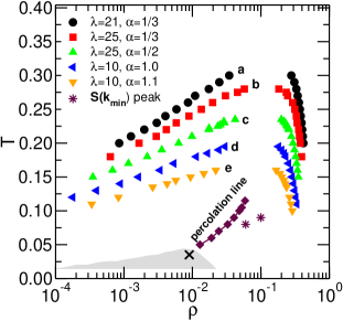
We describe the procedure by which the interaction parameters $\alpha$ and $\lambda$ have been chosen. Figure S1 shows the LG phase-coexistence curves, obtained from Gibbs Ensemble Monte Carlo (GEMC) simulationsPanagiotopoulos-gemc , for various combinations of $\lambda$ and $\alpha$. The GEMC simulations have been performed with $2000$ particles, with maximum step size of $0.085$. The values $\lambda=21$ and $\alpha=1/3$ represent silicon and the corresponding phase-coexistence curve is the same obtained by Honda et al.Honda . When $\lambda$ is increased to $25$ at constant $\alpha$ ($=1/3$), we find that the LG phase-coexistence curve moves to lower temperatures. Further, if $\alpha$ is increased to $1/2$ at fixed $\lambda~{}($=25$)$, the LG phase-coexistence curve shifts to even lower $T$’s. If we keep $\lambda$ fixed at $10$ and increase $\alpha$, the LG phase coexistence curve also moves to low $T$ and $\rho$ values. Thus increasing either $\lambda$ or $\alpha$ results in diminishing the LG coexistence region.

In addition to the effect on the LG coexistence, in order to ensure that the state of the system at intermediate densities is stable with respect to ordered structures (in our case, stackings of graphene-like sheets), we choose (among other possible choices) values $\lambda=10$ and $\alpha=1.49$ (further details may be found in shibu-thesis-suppl ).

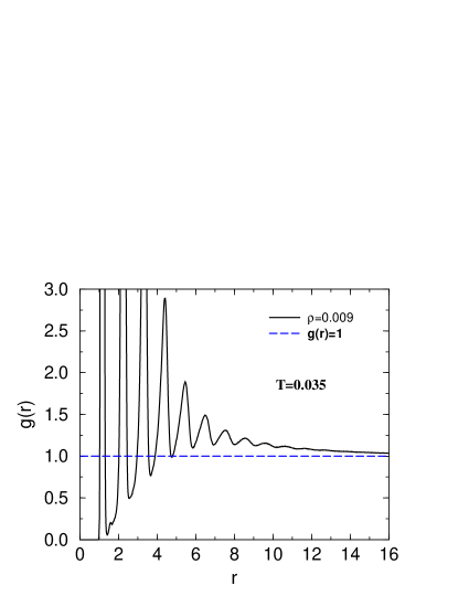
The LG phase coexistence curve for the values $\lambda=10$ and $\alpha=1.49$ can not be determined using GEMC simulations, because at low $T$ bonds become too strong to swap particles between two sub volumes, which is required for GEMC simulations. However, from Fig. S1 it is apparent that for $\lambda=10$ and $\alpha=1.49$, the LG phase-coexistence curve will be further suppressed compared to $\lambda=10$ and $\alpha=1.10$. A possible way to deduce the location of the LG coexistence region is to look for phase separation in a constant volume simulation. The shaded area in Fig. S1 shows the approximate region of LG phase coexistence for the present model from such MD simulations. However, the densities of both phases are very low, and therefore phase separation is not very easy to determine from the MD snapshots. Nevertheless, phase separation can be deduced by studying the radial distribution function, $g(r)$, which, if the system phase separates, approaches to $1.0$ from above instead of oscillating around $1.0$ at large distances, the behavior found in homogeneous systems. This behavior is shown in Fig. S2.

For completeness, we show in Fig. S1 also the percolation line. For a given temperature, the percolation density is determined as the density at which the percolation probability, estimated from considering several independent configurations, is $0.5$ (i.e. $50\%$ of the configurations have a spanning cluster of bonded particles). At the density $\rho=0.06$, which we study in detail, the percolation transition occurs at $T=0.115$.

Figure S2: The radial distribution function, $g(r)$, at density $\rho=0.009$ for $T=0.035$ (indicated by a cross in Fig. S1). The $g(r)$ approaches its large-$r$ limit from above, which indicates phase separation.

SII Static Properties

Figure S3: Snapshots of the system from MD simulations at density $0.06$ for: (a) $T=5.0$, (b) $T=0.08$, and (c) $T=0.028$.

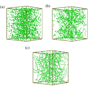
In order to get a first idea of the structure of the fluid, we show in Fig. S3 snapshots from the MD simulations at density $0.06$ and different temperatures. At a very high temperature, $T=5.0$ (Fig. S3a) the system is mainly composed of small sized clusters. Upon lowering the temperature, particles form an increasing number of interconnections, forming interlinked linear chains that percolate if $T$ is below 0.115. Figure S3b shows a snapshot at $T=0.08$ manifesting large heterogeneity, and the presence of significant voids, due to the proximity to the percolation point. At still lower temperatures, particles form increasingly longer, and stiffer, chains, and the system displays a more homogeneous morphology (see Fig. S3c for $T=0.028$). Therefore, at the lowest temperatures, the system consists mainly of linear chains of particles, with a small number of three-fold coordinated (“anchor”) particles connecting the linear chains.

SIII Wave-vector and Temperature Dependence of Dynamics

In Fig. S4 we show the coherent intermediate scattering function $F(k,t)$ vs. time for different $T$ and $k$ values obtained from MC as well as MD simulations. In order to allow to show the curves for different temperatures on the same graph, we plot the correlators as a function of $t/t_{\rm e}$, where $t_{\rm e}$ is the time at which the $F(k,t)$ reaches a value of $1/e$. From the graph we see that the relaxation behavior of $F(k,t)$ from the MC and MD simulations are quite different: Independent of $k$, the $F(k,t)$ from MC shows an exponential relaxation at the highest temperature shown ($T=0.10$), and becomes progressively more stretched as temperature decreases. On the other hand, MD simulations exhibit compressed exponential for all $T$, although a slower decay is apparent at lower $T$ due to the presence of acoustic modes. Thus we conclude that the MC dynamics suppresses the intermediate time compressed exponential behavior and allows one to see the stretched exponential decay at long times (see also Ref. shibuPRL-suppl ).

Last but not least we show in Fig. S5 the incoherent intermediate scattering function $F_{s}(k,t)$ vs. $t/t_{\rm se}$ for different $T$ and $k$ obtained from MC as well as MD simulations. The $F_{s}(k,t)$ curves from MC are nearly exponential at the lower $k$ values and higher $T$, showing stretching at the lowest $T$ for all $k$ values, and for all $T$ at $k=1.22$. The degree of stretching increases with decrease of $T$ and an increase of $k$. In contrast to this, $F_{s}(k,t)$ from MD shows a compressed exponential behavior for all $T$ at $k=1.22$, but at smaller $k$ the behavior becomes stretched at the two lowest temperatures (see main paper).

Figure S4: The collective intermediate scattering function $F(k,t)$ vs. time, for density = $0.06$, in log-linear scale as obtained from MD (dashed lines) and MC (solid lines) for (a) $k=0.62$ and (b) $k=1.22$.

Figure S5: The self intermediate scattering function $F_{s}(k,t)$ vs. time, for density = $0.06$, in log-linear scale as obtained from MD (dashed lines) and MC (solid lines) for (a) $k=0.62$ and (b) $k=1.22$.

SIV Cluster Size Distribution

Fig. S6 exhibits the cluster size distribution $n_{s}$ for different temperatures at density $0.06$. For very high temperatures $e.g.$, $T=5.0$, the $n_{s}$ shows an exponential decay, consistent with the possibility of a a random aggregation process. When the temperature is lowered, the distribution develops a slower than exponential decay. However, even for temperatures near the percolation transition, we do not find a distinguishable power-law regime, in contrast to the findings for other gel forming systems for which a power-law dependence corresponding to random percolation has been observed KobEuro-suppl ; Sciortino-ns-suppl ; Coniglio-ns-suppl .

Figure S6: The cluster size distribution $n_{s}$ for different temperature at density $0.06$. For very high temperature $T=5.0$ the $n_{s}$ shows an exponential form. At lower temperatures, including in the vicinity of the percolation transition, no distinguishable power-law regime is found, even though the cluster size distribution decays slower than exponentially.

References

- (1) S. Manley, B. Davidovitch, N. R. Davies, L. Cipelletti, A. E. Bailey, R. J. Christianson, U. Gasser, V. Prasad, P. N. Segre, M. P. Doherty, S. Sankaran, A. L. Jankovsky, B. Shiley, J. Bowen, J. Eggers, C. Kurta, T. Lorik, and D. A. Weitz, Phys. Rev. Lett. 95, 048302 (2005).
- (2) E. Zaccarelli, J. Phys.: Condens. Matter 19, 323101 (2007).
- (3) L. Cipelletti and L. Ramos, J. Phys.: Condens. Matter 17, R253 (2005).
- (4) E. Del Gado, A. Fierro, L. de Arcangelis, and A. Coniglio, Phys. Rev. E 69, 051103 (2004).
- (5) P. I. Hurtado, L. Berthier, and W. Kob, Phys. Rev. Lett. 98, 135503 (2007).
- (6) P. I. Hurtado, P. Chaudhuri, L. Berthier, and W. Kob, AIP Conf. Proc. 1091, 166 (2009).
- (7) R. Blaak, M. A. Miller, and J.-P. Hansen, Europhys. Lett. 78, 26002 (2007).
- (8) J. Russo, P. Tartaglia, and F. Sciortino, J. Chem. Phys. 131, 014504 (2009).
- (9) K. G. Soga, J. R. Melrose, and R. C. Ball, J. Chem. Phys. 108, 6026 (1998).
- (10) P. J. Lu, E. Zaccarelli, F. Ciulla, A. B. Schofield, F. Sciortino, and D.A. Weitz, Nature 453, 499 (2008).
- (11) S. Sastry, Phys. Rev. Lett., 85, 590 (2000).
- (12) E. Del Gado and W. Kob, Europhys. Lett. 72, 1032 (2005).
- (13) E. Zaccarelli, S.V. Buldyrev, E. La Nave, A. J. Moreno, I. Saika-Voivod, F. Sciortino, and P. Tartaglia, Phys. Rev. Lett. 94, 218301 (2005).
- (14) J. Bibette, T. G. Mason, H. Gang, and D. A. Weitz, Phys. Rev. Lett. 69, 981 (1992).
- (15) M.-A. Suarez, N. Kern, E. Pitard, and W. Kob, J. Chem. Phys. 130, 194904 (2009).
- (16) L. Cipelletti, S. Manley, R. C. Ball, and D. A. Weitz, Phys. Rev. Lett. 84, 2275 (2000).
- (17) R. Bandyopadhyay, D. Liang, H. Yardimci, D. A. Sessoms, M. A. Borthwick, S. G. J. Mochrie, J. L. Harden, and R. L. Leheny, Phys. Rev. Lett. 93, 228302 (2004).
- (18) K. Kroy, M. E. Cates, and W. C. K. Poon, Phys. Rev. Lett. 92, 148302 (2004).
- (19) E. Del Gado and W. Kob, Phys. Rev. Lett. 98, 028303 (2007).
- (20) A. Fierro, E. Del Gado, A. de Candia, and A. Coniglio, J. Stat. Mech., L04002 (2008).
- (21) E. Bianchi, J. Largo, P. Tartaglia, E. Zaccarelli, and F. Sciortino, Phys. Rev. Lett. 97, 168301 (2006).
- (22) F. Sciortino, Eur. Phys. J. B 64, 505 (2008).
- (23) S. Sastry, E. La Nave, and F. Sciortino, J. Stat. Mech., P12010, (2006).
- (24) B. Ruzicka et al, Nat. Mater. 10 56 (2010).
- (25) S. Saw, N. L. Ellegaard, W. Kob, and S. Sastry, Phys. Rev. Lett. 103, 248305 (2009).
- (26) F. H. Stillinger and T. A. Weber, Phys. Rev. B 31, 5262 (1985).
- (27) V. Molinero, S. Sastry, and C. A. Angell, Phys. Rev. Lett. 97, 075701 (2006).
- (28) S. Saw, Ph. D. Thesis, Jawaharlal Nehru Centre for Advanced Scientific Research (2010).
- (29) See Supplementary Material for details of how we choose the interaction parameters used in our study and how the phase-coexistence region gets suppressed. Also shown is the percolation line.
- (30) D. Brown and J. Clarke, Mol. Phys. 51, 1243 (1984).
- (31) M. P. Allen and D. J. Tildesley, Computer simulation of Liquids (Oxford University Press, Oxford, 1989).
- (32) R. Biswas and D. R. Hamann, Phys. Rev. Lett. 55, 2001 (1985).
- (33) T. A. Weber and F. H. Stillinger, Phys. Rev. E 48, 4351 (1993).
- (34) D. V. Makhov and L.J. Lewis, Phys. Rev. B 67, 153202 (2003).
- (35) D. Frenkel, Proceeding of the Workshop on Cellular Automata and Modelling of Complex Physical Systems, Les Houches, France, 21-18 February 1989, ed. P. Manneville (Springer, Berlin, 1989).
- (36) F. Sciortino, P. Tartaglia, and E. Zaccarelli, J. Phys. Chem. B 109, 21942 (2005).
- (37) E. Del Gado, L. de Arcangelis, and A. Coniglio, J. Phys. A: Math. Gen. 31, 1901 (1998).
- (38) In order to perform constrained MD simulations, we add a term of Gaussian form to the two-body potential that prevents the breaking of existing bonds or the formation of new ones. We use the values 30, 1.40 and 0.0001 as the prefactor, mean and variance of the imposed Gaussian potential. The Gaussian potential is shifted appropriately to nullify the discontinuity in the force arising due to truncation of the barrier potential.
- (39) W. Kob, C. Donati, S. J. Plimpton, P. H. Poole, and S. C. Glotzer, Phys. Rev. Lett. 79, 2827 (1997).
- (40) J. P. Boon and S. Yip, Molecular Hydrodynamics (Dover Publication, New York, 1979).
- (41) T. Odagaki and Y. Hiwatari, Phys. Rev. A 43, 1103 (1991.
- (42) W. Kob and H. C. Andersen, Phys. Rev. E 51, 4626 (1995).
- (43) F. Sciortino, P. Tartaglia, and E. Zaccarelli, J. Phys. Chem. B 109, 21942, 2005.
- (44) F. W. Starr, J. K. Nielsen, and H. E. Stanley, Phys. Rev. Lett. 82, 2294 (1999).
- (45) F. W. Starr, J. K. Nielsen, and H. E. Stanley, Phys. Rev. E 62, 579 (2000).
- (46) J. P. Hansen and I. R. McDonald, Theory of simple liquids; 2nd ed. (Academic Press, New York, 1986).
- (47) J.-P. Bouchaud and E. Pitard, Eur. Phys. J. E 9, 287 (2002).
- (48) W. Kob and H. C. Andersen, Phys. Rev. E 52, 4134 (1995).
- (49) T. Gleim, W. Kob, and K. Binder, Phys. Rev. Lett. 81, 4404 (1998).
- (50) L. Berthier, Phys. Rev. E 76, 011507 (2007).
- (51) L. Berthier and W. Kob, J. Phys.: Condens. Matter 19, 205130 (2007).
Supplementary Material
SI Choice of Interaction Parameters and
- (1) A. Z. Pangiotopolous, Mol. Phys. 61, 813 (1987).
- (2) N. Honda and Y.Nagasaka, Int. J. of Thermophysics 20, 837 (1999).
- (3) S. Saw, Ph. D. Thesis, Jawaharlal Nehru Centre for Advanced Scientific Research (2010).
- (4) S. Saw, N. L. Ellegaard, W. Kob, and S. Sastry, Phys. Rev. Lett. 103, 248305 (2009).
- (5) E. Del Gado and W. Kob, Europhys. Lett. 72, 1032 (2005).
- (6) F. Sciortino, P. Tartaglia, and E. Zaccarelli, J. Phys. Chem. B 109, 21942 (2005).
- (7) E. Del Gado, L. de Arcangelis, and A. Coniglio, J. Phys. A: Math. Gen. 31, 1901 (1998).