Geometrization of Three-Dimensional Orbifolds via Ricci Flow

Abstract.

A three-dimensional closed orientable orbifold (with no bad suborbifolds) is known to have a geometric decomposition from work of Perelman [50, 51] in the manifold case, along with earlier work of Boileau-Leeb-Porti [4], Boileau-Maillot-Porti [5], Boileau-Porti [6], Cooper-Hodgson-Kerckhoff [19] and Thurston [59]. We give a new, logically independent, unified proof of the geometrization of orbifolds, using Ricci flow. Along the way we develop some tools for the geometry of orbifolds that may be of independent interest.

1. Introduction

1.1. Orbifolds and geometrization

Thurston’s geometrization conjecture for $3$-manifolds states that every closed orientable $3$-manifold has a canonical decomposition into geometric pieces. In the early 1980’s Thurston announced a proof of the conjecture for Haken manifolds [60], with written proofs appearing much later [37, 42, 48, 49]. The conjecture was settled completely a few years ago by Perelman in his spectacular work using Hamilton’s Ricci flow [50, 51].

Thurston also formulated a geometrization conjecture for orbifolds. We recall that orbifolds are similar to manifolds, except that they are locally modelled on quotients of the form ${\mathbb{R}}^{n}/G$, where $G\subset O(n)$ is a finite subgroup of the orthogonal group. Although the terminology is relatively recent, orbifolds have a long history in mathematics, going back to the classification of crystallographic groups and Fuchsian groups. In this paper, using Ricci flow, we will give a new proof of the geometrization conjecture for orbifolds:

Theorem 1.1.

Let ${\mathcal{O}}$ be a closed connected orientable three-dimensional orbifold which does not contain any bad embedded $2$-dimensional suborbifolds. Then ${\mathcal{O}}$ has a geometric decomposition.

The existing proof of Theorem 1.1 is based on a canonical splitting of ${\mathcal{O}}$ along spherical and Euclidean $2$-dimensional suborbifolds, which is analogous to the prime and JSJ decomposition of $3$-manifolds. This splitting reduces Theorem 1.1 to two separate cases – when ${\mathcal{O}}$ is a manifold, and when ${\mathcal{O}}$ has a nonempty singular locus and satisfies an irreducibility condition. The first case is Perelman’s theorem for manifolds. Thurston announced a proof of the latter case in [59] and gave an outline. A detailed proof of the latter case was given by Boileau-Leeb-Porti [4], after work of Boileau-Maillot-Porti [5], Boileau-Porti [6], Cooper-Hodgson-Kerckhoff [19] and Thurston [59]. The monographs [5, 19] give excellent expositions of $3$-orbifolds and their geometrization.

1.2. Discussion of the proof

The main purpose of this paper is to provide a new proof of Theorem 1.1. Our proof is an extension of Perelman’s proof of geometrization for $3$-manifolds to orbifolds, bypassing [4, 5, 6, 19, 59]. The motivation for this alternate approach is twofold. First, anyone interested in the geometrization of general orbifolds as in Theorem 1.1 will necessarily have to go through Perelman’s Ricci flow proof in the manifold case, and also absorb foundational results about orbifolds. At that point, the additional effort required to deal with general orbifolds is relatively minor in comparison to the proof in [4]. This latter proof involves a number of ingredients, including Thurston’s geometrization of Haken manifolds, the deformation and collapsing theory of hyperbolic cone manifolds, and some Alexandrov space theory. Also, in contrast to the existing proof of Theorem 1.1, the Ricci flow argument gives a unified approach to geometrization for both manifolds and orbifolds.

Many of the steps in Perelman’s proof have evident orbifold generalizations, whereas some do not. It would be unwieldy to rewrite all the details of Perelman’s proof, on the level of [38], while making notational changes from manifolds to orbifolds. Consequently, we focus on the steps in Perelman’s proof where an orbifold extension is not immediate. For a step where the orbifold extension is routine, we make the precise orbifold statement and indicate where the analogous manifold proof occurs in [38].

In the course of proving Theorem 1.1, we needed to develop a number of foundational results about the geometry of orbifolds. Some of these may be of independent interest, or of use for subsequent work in this area, such as the compactness theorem for Riemannian orbifolds, critical point theory, and the soul theorem.

Let us mention one of the steps where the orbifold extension could a priori be an issue. This is where one characterizes the topology of the thin part of the large-time orbifold. To do this, one first needs a sufficiently flexible proof in the manifold case. We provided such a proof in [39]. The proof in [39] uses some basic techniques from Alexandrov geometry, combined with smoothness results in appropriate places. It provides a decomposition of the thin part into various pieces which together give an explicit realization of the thin part as a graph manifold. When combined with preliminary results that are proved in this paper, we can extend the techniques of [39] to orbifolds. We get a decomposition of the thin part of the large-time orbifold into various pieces, similar to those in [39]. We show that these pieces give an explicit realization of each component of the thin part as either a graph orbifold or one of a few exceptional cases. This is more involved to prove in the orbifold case than in the manifold case but the basic strategy is the same.

1.3. Organization of the paper

The structure of this paper is as follows. One of our tasks is to provide a framework for the topology and Riemannian geometry of orbifolds, so that results about Ricci flow on manifolds extend as easily as possible to orbifolds. In Section 2 we recall the relevant notions that we need from orbifold topology. We then introduce Riemannian orbifolds and prove the orbifold versions of some basic results from Riemannian geometry, such as the de Rham decomposition and critical point theory.

Section 3 is concerned with noncompact nonnegatively curved orbifolds. We prove the orbifold version of the Cheeger-Gromoll soul theorem. We list the diffeomorphism types of noncompact nonnegatively curved orbifolds with dimension at most three.

In Section 4 we prove a compactness theorem for Riemannian orbifolds. Section 5 contains some preliminary information about Ricci flow on orbifolds, along with the classification of the diffeomorphism types of compact nonnegatively curved three-dimensional orbifolds. We also show how to extend Perelman’s no local collapsing theorem to orbifolds.

Section 6 is devoted to $\kappa$-solutions. Starting in Section 7, we specialize to three-dimensional orientable orbifolds with no bad $2$-dimensional suborbifolds. We show how to extend Perelman’s results in order to construct a Ricci flow with surgery.

In Section 8 we show that the thick part of the large-time geometry approaches a finite-volume orbifold of constant negative curvature. Section 9 contains the topological characterization of the thin part of the large-time geometry.

Section 10 concerns the incompressibility of hyperbolic cross-sections. Rather than using minimal disk techniques as initiated by Hamilton [34], we follow an approach introduced by Perelman [51, Section 8] that uses a monotonic quantity, as modified in [38, Section 93.4].

The appendix contains topological facts about graph orbifolds. We show that a “weak” graph orbifold is the result of performing $0$-surgeries (i.e. connected sums) on a “strong” graph orbifold. This material is probably known to some experts but we were unable to find references in the literature, so we include complete proofs.

After writing this paper we learned that Daniel Faessler independently proved Proposition 9.7, which is the orbifold version of the collapsing theorem [24].

1.4. Acknowledgements

We thank Misha Kapovich and Sylvain Maillot for orbidiscussions. We thank the referee for a careful reading of the paper and for corrections.

2. Orbifold topology and geometry

In this section we first review the differential topology of orbifolds. Subsections 2.1 and 2.2 contain information about orbifolds in any dimension. In some cases we give precise definitions and in other cases we just recall salient properties, referring to the monographs [5, 19] for more detailed information. Subsections 2.3 and 2.4 are concerned with low-dimensional orbifolds.

We then give a short exposition of aspects of the differential geometry of orbifolds, in Subsection 2.5. It is hard to find a comprehensive reference for this material and so we flag the relevant notions; see [8] for further discussion of some points. Subsection 2.6 shows how to do critical point theory on orbifolds. Subsection 2.7 discusses the smoothing of functions on orbifolds.

For notation, $B^{n}$ is the open unit $n$-ball, $D^{n}$ is the closed unit $n$-ball and $I=[-1,1]$. We let $D_{k}$ denote the dihedral group of order $2k$.

2.1. Differential topology of orbifolds

An orbivector space is a triple $(V,G,\rho)$, where

• $V$ is a vector space,

• $G$ is a finite group and

• $\rho:G\rightarrow\operatorname{Aut}(V)$ is a faithful linear representation.

A (closed/ open/ convex/…) subset of $(V,G,\rho)$ is a $G$-invariant subset of $V$ which is (closed/ open/ convex/…) A linear map from $(V,G,\rho)$ to $(V^{\prime},G^{\prime},\rho^{\prime})$ consists of a linear map $T:V\rightarrow V^{\prime}$ and a homomorphism $h:G\rightarrow G^{\prime}$ so that for all $g\in G$, $\rho^{\prime}(h(g))\circ T=T\circ\rho(g)$. The linear map is injective (resp. surjective) if $T$ is injective (resp. surjective) and $h$ is injective (resp. surjective). An action of a group $K$ on $(V,G,\rho)$ is given by a short exact sequence $1\rightarrow G\rightarrow L\rightarrow K\rightarrow 1$ and a homomorphism $L\rightarrow\operatorname{Aut}(V)$ that extends $\rho$.

A local model is a pair $(\widehat{U},G)$, where $\widehat{U}$ is a connected open subset of a Euclidean space and $G$ is a finite group that acts smoothly and effectively on $\widehat{U}$, on the right. (Effectiveness means that the homomorphism $G\rightarrow\operatorname{Diff}(\widehat{U})$ is injective.) We will sometimes write $U$ for $\widehat{U}/G$, endowed with the quotient topology.

A smooth map between local models $(\widehat{U}_{1},G_{1})$ and $(\widehat{U}_{2},G_{2})$ is given by a smooth map $\widehat{f}\>:\>\widehat{U}_{1}\rightarrow\widehat{U}_{2}$ and a homomorphism $\rho\>:\>G_{1}\rightarrow G_{2}$ so that $\widehat{f}$ is $\rho$-equivariant, i.e. $\widehat{f}(xg_{1})\>=\>\widehat{f}(x)\rho(g_{1})$. We do not assume that $\rho$ is injective or surjective. The map between local models is an embedding if $\widehat{f}$ is an embedding; it follows from effectiveness that $\rho$ is injective in this case.

Definition 2.1.

An atlas for an $n$-dimensional orbifold ${\mathcal{O}}$ consists of
1. A Hausdorff paracompact topological space $|{\mathcal{O}}|$,
2. An open covering $\{U_{\alpha}\}$ of $|{\mathcal{O}}|$,
3. Local models $\{(\widehat{U}_{\alpha},G_{\alpha})\}$ with each $\widehat{U}_{\alpha}$ a connected open subset of ${\mathbb{R}}^{n}$ and
4. Homeomorphisms $\phi_{\alpha}\>:\>U_{\alpha}\rightarrow\widehat{U}_{\alpha}/G_{\alpha}$ so that
5. If $p\in U_{1}\cap U_{2}$ then there is a local model $(\widehat{U}_{3},G_{3})$ with $p\in U_{3}$ along with embeddings $(\widehat{U}_{3},G_{3})\rightarrow(\widehat{U}_{1},G_{1})$ and $(\widehat{U}_{3},G_{3})\rightarrow(\widehat{U}_{2},G_{2})$.

An orbifold ${\mathcal{O}}$ is an equivalence class of such atlases, where two atlases are equivalent if they are both included in a third atlas. With a given atlas, the orbifold ${\mathcal{O}}$ is oriented if each $\widehat{U}_{\alpha}$ is oriented, the action of $G_{\alpha}$ is orientation-preserving, and the embeddings $\widehat{U}_{3}\rightarrow\widehat{U}_{1}$ and $\widehat{U}_{3}\rightarrow\widehat{U}_{2}$ are orientation-preserving. We say that ${\mathcal{O}}$ is connected (resp. compact) if $|{\mathcal{O}}|$ is connected (resp. compact).

An orbifold-with-boundary ${\mathcal{O}}$ is defined similarly, with $\widehat{U}_{\alpha}$ being a connected open subset of $[0,\infty)\times{\mathbb{R}}^{n-1}$. The boundary $\partial{\mathcal{O}}$ is a boundaryless $(n-1)$-dimensional orbifold, with $|\partial{\mathcal{O}}|$ consisting of points in $|{\mathcal{O}}|$ whose local lifts lie in $\{0\}\times{\mathbb{R}}^{n-1}$. Note that it is possible that $\partial{\mathcal{O}}\>=\>\emptyset$ while $|{\mathcal{O}}|$ is a topological manifold with a nonempty boundary.

Remark 2.2.

In this paper we only deal with effective orbifolds, meaning that in a local model $(\widehat{U},G)$, the group $G$ always acts effectively. It would be more natural in some ways to remove this effectiveness assumption. However, doing so would hurt the readability of the paper, so we will stick to effective orbifolds.

Given a point $p\in|{\mathcal{O}}|$ and a local model $(\widehat{U},G)$ around $p$, let $\widehat{p}\in\widehat{U}$ project to $p$. The local group $G_{p}$ is the stabilizer group $\{g\in G\>:\>\widehat{p}g\>=\>\widehat{p}$ }. Its isomorphism class is independent of the choices made. We can always find a local model with $G=G_{p}$.

The regular part $|{\mathcal{O}}|_{reg}\subset|{\mathcal{O}}|$ consists of the points with $G_{p}\>=\>\{e\}$. It is a smooth manifold that forms an open dense subset of $|{\mathcal{O}}|$.

Given an open subset $X\subset|{\mathcal{O}}|$, there is an induced orbifold ${\mathcal{O}}\Big{|}_{X}$ with $\left|{\mathcal{O}}\Big{|}_{X}\right|=X$. In some cases we will have a subset $X\subset|{\mathcal{O}}|$, possibly not open, for which ${\mathcal{O}}\Big{|}_{X}$ is an orbifold-with-boundary.

The ends of ${\mathcal{O}}$ are the ends of $|{\mathcal{O}}|$.

A smooth map $f\>:\>{\mathcal{O}}_{1}\rightarrow{\mathcal{O}}_{2}$ between orbifolds is given by a continuous map $|f|\>:\>|{\mathcal{O}}_{1}|\rightarrow|{\mathcal{O}}_{2}|$ with the property that for each $p\in|{\mathcal{O}}_{1}|$, there are

• Local models $(\widehat{U}_{1},G_{1})$ and $(\widehat{U}_{2},G_{2})$ for $p$ and $f(p)$, respectively, and

• A smooth map $\widehat{f}\>:\>(\widehat{U}_{1},G_{1})\rightarrow(\widehat{U}_{2},G_{2})$ between local models

so that the diagram

(2.3) $$\begin{matrix}\widehat{U}_{1}&\stackrel{{\scriptstyle\widehat{f}}}{{\rightarrow}}&\widehat{U}_{2}\\ \downarrow&&\downarrow\\ U_{1}&\stackrel{{\scriptstyle|f|}}{{\rightarrow}}&U_{2}\end{matrix}$$

commutes.

There is an induced homomorphism from $G_{p}$ to $G_{f(p)}$. We emphasize that to define a smooth map $f$ between two orbifolds, one must first define a map $|f|$ between their underlyihg spaces.

We write $C^{\infty}({\mathcal{O}})$ for the space of smooth maps $f:{\mathcal{O}}\rightarrow{\mathbb{R}}$.

A smooth map $f:{\mathcal{O}}_{1}\rightarrow{\mathcal{O}}_{2}$ is proper if $|f|:|{\mathcal{O}}_{1}|\rightarrow|{\mathcal{O}}_{2}|$ is a proper map.

A diffeomorphism $f\>:\>{\mathcal{O}}_{1}\rightarrow{\mathcal{O}}_{2}$ is a smooth map with a smooth inverse. Then $G_{p}$ is isomorphic to $G_{f(p)}$.

If a discrete group $\Gamma$ acts properly discontinuously on a manifold $M$ then there is a quotient orbifold, which we denote by $M//\Gamma$. It has $|M//\Gamma|=M/\Gamma$. Hence if ${\mathcal{O}}$ is an orbifold and $(\widehat{U},G)$ is a local model for ${\mathcal{O}}$ then we can say that ${\mathcal{O}}\Big{|}_{U}$ is diffeomorphic to $\widehat{U}//G$. An orbifold ${\mathcal{O}}$ is good if ${\mathcal{O}}=M//\Gamma$ for some manifold $M$ and some discrete group $\Gamma$. It is very good if $\Gamma$ can be taken to be finite. A bad orbifold is one that is not good.

Similarly, suppose that a discrete group $\Gamma$ acts by diffeomorphisms on an orbifold ${\mathcal{O}}$. We say that it acts properly discontinuously if the action of $\Gamma$ on $|{\mathcal{O}}|$ is properly discontinuous. Then there is a quotient orbifold ${\mathcal{O}}//\Gamma$, with $|{\mathcal{O}}//\Gamma|=|{\mathcal{O}}|/\Gamma$; see Remark 2.15.

An orbifiber bundle consists of a smooth map $\pi:{\mathcal{O}}_{1}\rightarrow{\mathcal{O}}_{2}$ between two orbifolds, along with a third orbifold ${\mathcal{O}}_{3}$ such that

• $|\pi|$ is surjective, and

• For each $p\in|{\mathcal{O}}_{2}|$, there is a local model $(\widehat{U},G_{p})$ around $p$, where $G_{p}$ is the local group at $p$, along with an action of $G_{p}$ on ${\mathcal{O}}_{3}$ and a diffeomorphism $({\mathcal{O}}_{3}\times\widehat{U})//G_{p}\rightarrow{\mathcal{O}}_{1}\Big{|}_{|\pi|^{-1}(U)}$ so that the diagram

  (2.4) $$\begin{matrix}({\mathcal{O}}_{3}\times\widehat{U})//G_{p}&\rightarrow&{\mathcal{O}}_{1}\\ \downarrow&&\downarrow\\ \widehat{U}//G_{p}&\rightarrow&{\mathcal{O}}_{2}\end{matrix}$$

  commutes.

(Note that if ${\mathcal{O}}_{2}$ is a manifold then the orbifiber bundle $\pi:{\mathcal{O}}_{1}\rightarrow{\mathcal{O}}_{2}$ has a local product structure.) The fiber of the orbifiber bundle is ${\mathcal{O}}_{3}$. Note that for $p_{1}\in|{\mathcal{O}}_{1}|$, the homomorphism $G_{p_{1}}\rightarrow G_{|\pi|(p_{1})}$ is surjective.

A section of an orbifiber bundle $\pi:{\mathcal{O}}_{1}\rightarrow{\mathcal{O}}_{2}$ is a smooth map $s:{\mathcal{O}}_{2}\rightarrow{\mathcal{O}}_{1}$ such that $\pi\circ s$ is the identity on ${\mathcal{O}}_{2}$.

A covering map $\pi:{\mathcal{O}}_{1}\rightarrow{\mathcal{O}}_{2}$ is a orbifiber bundle with a zero-dimensional fiber. Given $p_{2}\in|{\mathcal{O}}_{2}|$ and $p_{1}\in|\pi|^{-1}(p_{2})$, there are a local model $(\widehat{U},G_{2})$ around $p_{2}$ and a subgroup $G_{1}\subset G_{2}$ so that $(\widehat{U},G_{1})$ is a local model around $p_{1}$ and the map $\pi$ is locally $(\widehat{U},G_{1})\rightarrow(\widehat{U},G_{2})$.

A rank-$m$ orbivector bundle ${\mathcal{V}}\rightarrow{\mathcal{O}}$ over ${\mathcal{O}}$ is locally isomorphic to $(V\times\widehat{U})/G_{p}$, where $V$ is an $m$-dimensional orbivector space on which $G_{p}$ acts linearly.

The tangent bundle $T{\mathcal{O}}$ of an orbifold ${{\mathcal{O}}}$ is an orbivector bundle which is locally diffeomorphic to $T\widehat{U}_{\alpha}//G_{\alpha}$. Given $p\in|{\mathcal{O}}|$, if $\widehat{p}\in\widehat{U}$ covers $p$ then the tangent space $T_{p}{\mathcal{O}}$ is isomorphic to the orbivector space $(T_{\widehat{p}}\widehat{U},G_{p})$. The tangent cone at $p$ is $C_{p}|{\mathcal{O}}|\cong T_{\widehat{p}}\widehat{U}/G_{p}$.

A smooth vector field $V$ is a smooth section of $T{\mathcal{O}}$. In terms of a local model $(\widehat{U},G)$, the vector field $V$ restricts to a vector field on $\widehat{U}$ which is $G$-invariant.

A smooth map $f:{\mathcal{O}}_{1}\rightarrow{\mathcal{O}}_{2}$ gives rise to the differential, an orbivector bundle map $df:T{\mathcal{O}}_{1}\rightarrow T{\mathcal{O}}_{2}$. At a point $p\in|{\mathcal{O}}|$, in terms of local models we have a map $\widehat{f}:(\widehat{U}_{1},G_{1})\rightarrow(\widehat{U}_{2},G_{2})$ which gives rise to a $G_{p}$-equivariant map $d\widehat{f}_{p}:T_{\widehat{p}}\widehat{U}_{1}\rightarrow T_{\widehat{f}(\widehat{p})}\widehat{U}_{2}$ and hence to a linear map $df_{p}:T_{p}{\mathcal{O}}_{1}\rightarrow T_{|f|(p)}{\mathcal{O}}_{2}$.

Given a smooth map $f:{\mathcal{O}}_{1}\rightarrow{\mathcal{O}}_{2}$ and a point $p\in|{\mathcal{O}}_{1}|$, we say that $f$ is a submersion at $p$ (resp. immersion at $p$) if the map $df_{p}:T_{p}{\mathcal{O}}_{1}\rightarrow T_{|f|(p)}{\mathcal{O}}_{2}$ is surjective (resp. injective).

Lemma 2.5.

If $f$ is a submersion at $p$ then there is an orbifold ${\mathcal{O}}_{3}$ on which $G_{|f|(p)}$ acts, along with a local model $(\widehat{U}_{2},G_{|f|(p)})$ around $|f|(p)$, so that $f$ is equivalent near $p$ to the projection map $({\mathcal{O}}_{3}\times\widehat{U}_{2})//G_{|f|(p)}\rightarrow\widehat{U}_{2}//G_{|f|(p)}$.

Proof.

Let $\rho:G_{p}\rightarrow G_{|f|(p)}$ be the surjective homomorphism associated to $df_{p}$. Let $\widehat{f}\>:\>(\widehat{U}_{1},G_{p})\rightarrow(\widehat{U}_{2},G_{|f|(p)})$ be a local model for $f$ near $p$; it is necessarily $\rho$-equivariant. Let $\widehat{p}\in\widehat{U}_{1}$ be a lift of $p\in U_{1}$. Put $\widehat{W}=\widehat{f}^{-1}(\widehat{f}(\widehat{p}))$. Since $\widehat{f}$ is a submersion at $\widehat{p}$, after reducing $\widehat{U}_{1}$ and $\widehat{U}_{2}$ if necessary, there is a $\rho$-equivariant diffeomorphism $\widehat{W}\times\widehat{U}_{2}\rightarrow\widehat{U}_{1}$ so that the diagram

(2.6) $$\begin{matrix}\widehat{W}\times\widehat{U}_{2}&\rightarrow&\widehat{U}_{1}\\ \downarrow&&\downarrow\\ \widehat{U}_{2}&\rightarrow&\widehat{U}_{2}\end{matrix}$$

commutes and is $G_{p}$-equivariant. Now $\operatorname{Ker}(\rho)$ acts on $\widehat{W}$. Put ${\mathcal{O}}_{3}=\widehat{W}//\operatorname{Ker}(\rho)$. Then there is a commuting diagram of orbifold maps

(2.7) $$\begin{matrix}{\mathcal{O}}_{3}\times\widehat{U}_{2}&\rightarrow&\widehat{U}_{1}//\operatorname{Ker}(\rho)\\ \downarrow&&\downarrow\\ \widehat{U}_{2}&\rightarrow&\widehat{U}_{2}\end{matrix}.$$

Further quotienting by $G_{|f|(p)}$ gives a commutative diagram

(2.8) $$\begin{matrix}({\mathcal{O}}_{3}\times\widehat{U}_{2})//G_{|f|(p)}&\rightarrow&\widehat{U}_{1}//G_{p}\\ \downarrow&&\downarrow\\ \widehat{U}_{2}//G_{|f|(p)}&\rightarrow&\widehat{U}_{2}//G_{|f|(p)}\end{matrix}$$

whose top horizontal line is an orbifold diffeomorphism. ∎

We say that $f:{\mathcal{O}}_{1}\rightarrow{\mathcal{O}}_{2}$ is a submersion (resp. immersion) if it is a submersion (resp. immersion) at $p$ for all $p\in|{\mathcal{O}}_{1}|$.

Lemma 2.9.

A proper surjective submersion $f:{\mathcal{O}}_{1}\rightarrow{\mathcal{O}}_{2}$, with ${\mathcal{O}}_{2}$ connected, defines an orbifiber bundle with compact fibers.

We will sketch a proof of Lemma 2.9 in Remark 2.17.

In particular, a proper surjective local diffeomorphism to a connected orbifold is a covering map with finite fibers.

An immersion $f:{\mathcal{O}}_{1}\rightarrow{\mathcal{O}}_{2}$ has a normal bundle $N{\mathcal{O}}_{1}\rightarrow{\mathcal{O}}_{1}$ whose fibers have the following local description. Given $p\in|{\mathcal{O}}_{1}|$, let $f$ be described in terms of local models $(\widehat{U}_{1},G_{p})$ and $(\widehat{U}_{2},G_{|f|(p)})$ by a $\rho$-equivariant immersion $\widehat{f}\>:\>\widehat{U}_{1}\rightarrow\widehat{U}_{2}$. Let $F_{p}\subset G_{|f|(p)}$ be the subgroup which fixes $\operatorname{Im}(d\widehat{f}_{p})$. Then the normal space $N_{p}{\mathcal{O}}_{1}$ is the orbivector space $\left(\operatorname{Coker}(d\widehat{f}_{p}),F_{p}\right)$.

A suborbifold of ${\mathcal{O}}$ is given by an orbifold ${\mathcal{O}}^{\prime}$ and an immersion $f:{\mathcal{O}}^{\prime}\rightarrow{\mathcal{O}}$ for which $|f|$ maps $|{\mathcal{O}}^{\prime}|$ homeomorphically to its image in $|{\mathcal{O}}|$. From effectiveness, for each $p\in|{\mathcal{O}}^{\prime}|$, the homomorphism $\rho_{p}:G_{p}\rightarrow G_{|f|(p)}$ is injective. Note that $\rho_{p}$ need not be an isomorphism. We will identify ${\mathcal{O}}^{\prime}$ with its image in ${\mathcal{O}}$. There is a neighborhood of ${\mathcal{O}}^{\prime}$ which is diffeomorphic to the normal bundle $N{\mathcal{O}}^{\prime}$. We say that the suborbifold ${\mathcal{O}}^{\prime}$ is embedded if ${\mathcal{O}}\Big{|}_{|{\mathcal{O}}^{\prime}|}={\mathcal{O}}^{\prime}$. Then for each $p\in|{\mathcal{O}}^{\prime}|$, the homomorphism $\rho_{p}$ is an isomorphism.

If ${\mathcal{O}}^{\prime}$ is an embedded codimension-$1$ suborbifold of ${\mathcal{O}}$ then we say that ${\mathcal{O}}^{\prime}$ is two-sided if the normal bundle $N{\mathcal{O}}^{\prime}$ has a nowhere-zero section. If ${\mathcal{O}}$ and ${\mathcal{O}}^{\prime}$ are both orientable then ${\mathcal{O}}^{\prime}$ is two-sided. We say that ${\mathcal{O}}^{\prime}$ is separating if $|{\mathcal{O}}^{\prime}|$ is separating in $|{\mathcal{O}}|$.

We can talk about two suborbifolds meeting transversely, as defined using local models.

Let ${\mathcal{O}}$ be an oriented orbifold (possibly disconnected). Let $D_{1}$ and $D_{2}$ be disjoint codimension-zero embedded suborbifolds-with-boundary, both oriented-diffeomorphic to $D^{n}//\Gamma$. Then the operation of performing $0$-surgery along $D_{1}$, $D_{2}$ produces the new oriented orbifold ${\mathcal{O}}^{\prime}=({\mathcal{O}}-\operatorname{int}(D_{1})-\operatorname{int}(D_{2}))\bigcup_{\partial D_{1}\sqcup\partial D_{2}}(I\times(D^{n}//\Gamma))$. In the manifold case, a connected sum is the same thing as a $0$-surgery along a pair $\{D_{1},D_{2}\}$ which lie in different connected components of ${\mathcal{O}}$. Note that unlike in the manifold case, ${\mathcal{O}}^{\prime}$ is generally not uniquely determined up to diffeomorphism by knowing the connected components containing $D_{1}$ and $D_{2}$. For example, even if ${\mathcal{O}}$ is connected, $D_{1}$ and $D_{2}$ may or may not lie on the same connected component of the singular set.

If ${\mathcal{O}}_{1}$ and ${\mathcal{O}}_{2}$ are oriented orbifolds, with $D_{1}\subset{\mathcal{O}}_{1}$ and $D_{2}\subset{\mathcal{O}}_{2}$ both oriented diffeomorphic to $D^{n}//\Gamma$, then we may write ${\mathcal{O}}_{1}\#_{S^{n-1}//\Gamma}{\mathcal{O}}_{2}$ for the connected sum. This notation is slightly ambiguous since the location of $D_{1}$ and $D_{2}$ is implicit. We will write ${\mathcal{O}}\#_{S^{n-1}//\Gamma}$ to denote a $0$-surgery on a single orbifold ${\mathcal{O}}$. Again the notation is slightly ambiguous, since the location of $D_{1},D_{2}\subset{\mathcal{O}}$ is implicit.

An involutive distribution on ${\mathcal{O}}$ is a subbundle $E\subset T{\mathcal{O}}$ with the property that for any two sections $V_{1},V_{2}$ of $E$, the Lie bracket $[V_{1},V_{2}]$ is also a section of $E$.

Lemma 2.10.

Given an involutive distribution $E$ on ${\mathcal{O}}$, for any $p\in|{\mathcal{O}}|$ there is a unique maximal suborbifold passing through $p$ which is tangent to $E$.

Orbifolds have partitions of unity.

Lemma 2.11.

Given an open cover $\{U_{\alpha}\}_{\alpha\in A}$ of $|{\mathcal{O}}|$, there is a collection of functions $\rho_{\alpha}\in C^{\infty}({\mathcal{O}})$ such that

• $0\leq\rho_{\alpha}\leq 1$.

• $\operatorname{supp}(\rho_{\alpha})\subset U_{\alpha^{\prime}}$ for some $\alpha^{\prime}=\alpha^{\prime}(\alpha)\in A$.

• For all $p\in|{\mathcal{O}}|$, $\sum_{\alpha\in A}\rho_{\alpha}(p)=1$.

Proof.

The proof is similar to the manifold case, using local models $(\widehat{U},G)$ consisting of coordinate neighborhoods, along with compactly supported $G$-invariant smooth functions on $\widehat{U}$. ∎

A curve in an orbifold is a smooth map $\gamma\>:\>I\rightarrow{\mathcal{O}}$ defined on an interval $I\subset{\mathbb{R}}$. A loop is a curve $\gamma$ with $|\gamma|(0)=|\gamma|(1)\in|{\mathcal{O}}|$.

2.2. Universal cover and fundamental group

We follow the presentation in [5, Chapter 2.2.1]. Choose a regular point $p\in|{\mathcal{O}}|$. A special curve from $p$ is a curve $\gamma:[0,1]\rightarrow{\mathcal{O}}$ such that

• $|\gamma|(0)=p$ and

• $|\gamma|(t)$ lies in $|{\mathcal{O}}|_{reg}$ for all but a finite number of $t$.

Suppose that $(\widehat{U},G)$ is a local model and that $\widehat{\gamma}:[a,b]\rightarrow\widehat{U}$ is a lifting of $\gamma_{[a,b]}$, for some $[a,b]\subset[0,1]$. An elementary homotopy between two special curves is a smooth homotopy of $\widehat{\gamma}$ in $\widehat{U}$, relative to $\widehat{\gamma}(a)$ and $\widehat{\gamma}(b)$. A homotopy of $\gamma$ is what’s generated by elementary homotopies.

If ${\mathcal{O}}$ is connected then the universal cover $\widetilde{{\mathcal{O}}}$ of ${\mathcal{O}}$ can be constructed as the set of special curves starting at $p$, modulo homotopy. It has a natural orbifold structure. The fundamental group $\pi_{1}({\mathcal{O}},p)$ is given by special loops (i.e. special curves $\gamma$ with $|\gamma|(1)=p$) modulo homotopy. Up to isomorphism, $\pi_{1}({\mathcal{O}},p)$ is independent of the choice of $p$.

If ${\mathcal{O}}$ is connected and a discrete group $\Gamma$ acts properly discontinuously on ${\mathcal{O}}$ then there is a short exact sequence

(2.12) $$1\longrightarrow\pi_{1}({\mathcal{O}},p)\longrightarrow\pi_{1}({\mathcal{O}}//\Gamma,p\Gamma)\longrightarrow\Gamma\longrightarrow 1.$$

Remark 2.13.

A more enlightening way to think of an orbifold is to consider it as a smooth effective proper étale groupoid ${\mathcal{G}}$, as explained in [1, 12, 45]. We recall that a Lie groupoid ${\mathcal{G}}$ essentially consists of a smooth manifold ${\mathcal{G}}^{(0)}$ (the space of units), another smooth manifold ${\mathcal{G}}^{(1)}$ and submersions $s,r:{\mathcal{G}}^{(1)}\rightarrow{\mathcal{G}}^{(0)}$ (the source and range maps), along with a partially defined multiplication ${\mathcal{G}}^{(1)}\times{\mathcal{G}}^{(1)}\rightarrow{\mathcal{G}}^{(1)}$ which satisfies certain compatibility conditions. A Lie groupoid is étale if $s$ and $r$ are local diffeomorphisms. It is proper if $(s,r):{\mathcal{G}}^{(1)}\rightarrow{\mathcal{G}}^{(0)}\times{\mathcal{G}}^{(0)}$ is a proper map. There is also a notion of an étale groupoid being effective.

To an orbifold one can associate an effective proper étale groupoid as follows. Given an orbifold ${\mathcal{O}}$, a local model $(\widehat{U}_{\alpha},G_{\alpha})$ and some $\widehat{p}_{\alpha}\in\widehat{U}_{\alpha}$, let $p\in|{\mathcal{O}}|$ be the corresponding point. There is a quotient map $A_{\widehat{p}_{\alpha}}:T_{\widehat{p}_{\alpha}}\widehat{U}_{\alpha}\rightarrow C_{p}|{\mathcal{O}}|$. The unit space ${\mathcal{G}}^{(0)}$ is the disjoint union of the $\widehat{U}_{\alpha}$’s. And ${\mathcal{G}}^{(1)}$ consists of the triples $(\widehat{p}_{\alpha},\widehat{p}_{\beta},B_{\widehat{p}_{\alpha},\widehat{p}_{\beta}})$ where

1. $\widehat{p}_{\alpha}\in\widehat{U}_{\alpha}$ and $\widehat{p}_{\beta}\in\widehat{U}_{\beta}$,

2. $\widehat{p}_{\alpha}$ and $\widehat{p}_{\beta}$ map to the same point $p\in|{\mathcal{O}}|$ and

3. $B_{\widehat{p}_{\alpha},\widehat{p}_{\beta}}:T_{\widehat{p}_{\alpha}}\widehat{U}_{\alpha}\rightarrow T_{\widehat{p}_{\beta}}\widehat{U}_{\beta}$ is an invertible linear map so that $A_{\widehat{p}_{\alpha}}=A_{\widehat{p}_{\beta}}\circ B_{\widehat{p}_{\alpha},\widehat{p}_{\beta}}$.

There is an obvious way to compose triples $(\widehat{p}_{\alpha},\widehat{p}_{\beta},B_{\widehat{p}_{\alpha},\widehat{p}_{\beta}})$ and $(\widehat{p}_{\beta},\widehat{p}_{\gamma},B_{\widehat{p}_{\beta},\widehat{p}_{\gamma}})$. One can show that this gives rise to a smooth effective proper étale groupoid.

Conversely, given a smooth effective proper étale groupoid ${\mathcal{G}}$, for any $\widehat{p}\in{\mathcal{G}}^{(0)}$ the isotropy group ${\mathcal{G}}_{\widehat{p}}^{\widehat{p}}$ is a finite group. To get an orbifold, one can take local models of the form $(\widehat{U},{\mathcal{G}}_{\widehat{p}}^{\widehat{p}})$ where $\widehat{U}$ is a ${\mathcal{G}}_{\widehat{p}}^{\widehat{p}}$-invariant neighborhood of $\widehat{p}$.

Speaking hereafter just of smooth effective proper étale groupoids, Morita-equivalent groupoids give equivalent orbifolds.

A groupoid morphism gives rise to an orbifold map. Taking into account Morita equivalence, from the groupoid viewpoint the right notion of an orbifold map would be a Hilsum-Skandalis map between groupoids. These turn out to correspond to good maps between orbifolds, as later defined by Chen-Ruan [1]. This is a more restricted class of maps between orbifolds than what we consider. The distinction is that one can pull back orbivector bundles under good maps, but not always under smooth maps in our sense. Orbifold diffeomorphisms in our sense are automatically good maps. For some purposes it would be preferable to only deal with good maps, but for simplicity we will stick with our orbifold definitions.

A Lie groupoid ${\mathcal{G}}$ has a classifying space $B{\mathcal{G}}$. In the orbifold case, if ${\mathcal{G}}$ is the étale groupoid associated to an orbifold ${\mathcal{O}}$ then $\pi_{1}({\mathcal{O}})\cong\pi_{1}(B{\mathcal{G}})$. The definition of the latter can be made explicit in terms of paths and homotopies; see [12, 29]. In the case of effective orbifolds, the definition is equivalent to the one of the present paper.

More information is in [1, 45] and references therein.

2.3. Low-dimensional orbifolds

We list the connected compact boundaryless orbifolds of low dimension. We mostly restrict here to the orientable case. (The nonorientable ones also arise; even if the total space of an orbifiber bundle is orientable, the base may fail to be orientable.)

2.3.1. Zero dimensions

The only possibility is a point.

2.3.2. One dimension

There are two possibilities : $S^{1}$ and $S^{1}//{\mathbb{Z}}_{2}$. For the latter, the nonzero element of ${\mathbb{Z}}_{2}$ acts by complex conjugation on $S^{1}$, and $|S^{1}//{\mathbb{Z}}_{2}|$ is an interval. Note that $S^{1}//{\mathbb{Z}}_{2}$ is not orientable.

2.3.3. Two dimensions

For notation, if $S$ is a connected oriented surface then $S(k_{1},\ldots,k_{r})$ denotes the oriented orbifold ${\mathcal{O}}$ with $|{\mathcal{O}}|=S$, having singular points of order $k_{1},\ldots,k_{r}>1$. Any connected oriented $2$-orbifold can be written in this way. An orbifold of the form $S^{2}(p,q,r)$ is called a turnover.

The bad orientable $2$-orbifolds are $S^{2}(k)$ and $S^{2}(k,k^{\prime})$, $k\neq k^{\prime}$. The latter is simply-connected if and only if $\gcd(k,k^{\prime})=1$.

The spherical $2$-orbifolds are of the form $S^{2}//\Gamma$, where $\Gamma$ is a finite subgroup of $\operatorname{Isom}^{+}(S^{2})$. The orientable ones are $S^{2}$, $S^{2}(k,k)$, $S^{2}(2,2,k)$, $S^{2}(2,3,3)$, $S^{2}(2,3,4)$, $S^{2}(2,3,5)$. (If $S^{2}(1,1)$ arises in this paper then it means $S^{2}$.)

The Euclidean $2$-orbifolds are of the form $T^{2}//\Gamma$, where $\Gamma$ is a finite subgroup of $\operatorname{Isom}^{+}(T^{2})$. The orientable ones are $T^{2}$, $S^{2}(2,3,6)$, $S^{2}(2,4,4)$, $S^{2}(3,3,3)$, $S^{2}(2,2,2,2)$. The latter is called a pillowcase and can be identified with the quotient of $T^{2}={\mathbb{C}}/{\mathbb{Z}}^{2}$ by ${\mathbb{Z}}_{2}$, where the action of the nontrivial element of ${\mathbb{Z}}_{2}$ comes from the map $z\rightarrow-z$ on ${\mathbb{C}}$.

The other closed orientable $2$-orbifolds are hyperbolic.

We will also need some $2$-orbifolds with boundary, namely

• The discal $2$-orbifolds $D^{2}(k)=D^{2}//{\mathbb{Z}}_{k}$.

• The half-pillowcase $D^{2}(2,2)=I\times_{{\mathbb{Z}}_{2}}S^{1}$. Here the nontrivial element of ${\mathbb{Z}}_{2}$ acts by involution on $I$ and by complex conjugation on $S^{1}$. We can also write $D^{2}(2,2)$ as the quotient $\{z\in{\mathbb{C}}\>:\>\frac{1}{2}\leq|z|\leq 2\}//{\mathbb{Z}}_{2}$, where the nontrivial element of ${\mathbb{Z}}_{2}$ sends $z$ to $z^{-1}$.

• $D^{2}//{\mathbb{Z}}_{2}$, where ${\mathbb{Z}}_{2}$ acts by complex conjugation on $D^{2}$. Then $\partial|D^{2}//{\mathbb{Z}}_{2}|$ is a circle with one orbifold boundary component and one reflector component. See Figure 1, where the dark line indicates the reflector component.

  

  Figure 1.

  

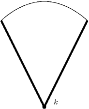
  Figure 2.

  

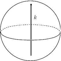
  Figure 3.

• $D^{2}//D_{k}=D^{2}(k)//{\mathbb{Z}}_{2}$, for $k>1$, where $D_{k}$ is the dihedral group and ${\mathbb{Z}}_{2}$ acts by complex conjugation on $D^{2}(k)$. Then $\partial|D^{2}//D_{k}|$ is a circle with one orbifold boundary component, one corner reflector point of order $k$ and two reflector components. See Figure 2.

2.3.4. Three dimensions

If ${\mathcal{O}}$ is an orientable three-dimensional orbifold then $|{\mathcal{O}}|$ is an orientable topological $3$-manifold. If ${\mathcal{O}}$ is boundaryless then $|{\mathcal{O}}|$ is boundaryless. Each component of the singular locus in $|{\mathcal{O}}|$ is either

1. a knot or arc (with endpoints on $\partial|{\mathcal{O}}|$), labelled by an integer greater than one, or

2. a trivalent graph with each edge labelled by an integer greater than one, under the constraint that if edges with labels $p,q,r$ meet at a vertex then $\frac{1}{p}+\frac{1}{q}+\frac{1}{r}>1$. That is, there is a neighborhood of the vertex which is a cone over an orientable spherical $2$-orbifold.

Specifying such a topological $3$-manifold and such a labelled graph is equivalent to specifying an orientable three-dimensional orbifold.

We write $D^{3}//\Gamma$ for a discal $3$-orbifold whose boundary is $S^{2}//\Gamma$. They are

• $D^{3}$. There is no singular locus.

• $D^{3}(k,k)$. The singular locus is a line segment through $D^{3}$. See Figure 3.

• $D^{3}(2,2,k)$, $D^{3}(2,3,3)$, $D^{3}(2,3,4)$ and $D^{3}(2,3,5)$. The singular locus is a tripod in $D^{3}$. See Figure 4.

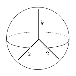
Figure 4.

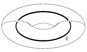
Figure 5.

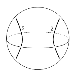
Figure 6.

The solid-toric $3$-orbifolds are

• $S^{1}\times D^{2}$. There is no singular locus.

• $S^{1}\times D^{2}(k)$. The singular locus is a core curve in a solid torus. See Figure 5

• $S^{1}\times_{Z_{2}}D^{2}$. The singular locus consists of two arcs in a $3$-disk, each labelled by $2$. The boundary is $S^{2}(2,2,2,2)$. See Figure 6.

• $S^{1}\times_{Z_{2}}D^{2}(k)$. The singular locus consists of two arcs in a $3$-disk, each labelled by $2$, joined in their middles by an arc labelled by $k$. The boundary is $S^{2}(2,2,2,2)$. See Figure 7.

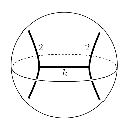
Figure 7.

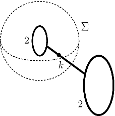
Figure 8.

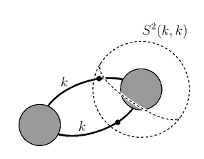
Figure 9. An essential spherical suborbifold

Given $\Gamma\in\operatorname{Isom}^{+}(S^{2})$, we can consider the quotient $S^{3}//\Gamma$ where $\Gamma$ acts on $S^{3}$ by the suspension of its action on $S^{2}$. That is, we are identifying $\operatorname{Isom}^{+}(S^{2})$ with $\operatorname{SO}(3)$ and using the embedding $\operatorname{SO}(3)\rightarrow\operatorname{SO}(4)$ to let $\Gamma$ act on $S^{3}$.

An orientable three-dimensional orbifold ${\mathcal{O}}$ is irreducible if it contains no embedded bad $2$-dimensional suborbifolds, and any embedded orientable spherical $2$-orbifold $S^{2}//\Gamma$ bounds a discal $3$-orbifold $D^{3}//\Gamma$ in ${\mathcal{O}}$. Figure 8 shows an embedded bad $2$-dimensional suborbifold $\Sigma$. Figure 9 shows an embedded spherical $2$-suborbifold $S^{2}(k,k)$ that does not bound a discal $3$-orbifold; the shaded regions are meant to indicate some complicated orbifold regions.

If $S$ is an orientable embedded $2$-orbifold in ${\mathcal{O}}$ then $S$ is compressible if there is an embedded discal 2-orbifold $D\subset{\mathcal{O}}$ so that $\partial D$ lies in $S$, but $\partial D$ does not bound a discal $2$-orbifold in $S$. (We call $D$ a compressing discal orbifold.) Otherwise, $S$ is incompressible. Note that any embedded copy of a turnover $S^{2}(p,q,r)$ is automatically incompressible, since any embedded circle in $S^{2}(p,q,r)$ bounds a discal $2$-orbifold in $S^{2}(p,q,r)$.

If ${\mathcal{O}}$ is a compact orientable $3$-orbifold then there is a compact orientable irreducible $3$-orbifold ${\mathcal{O}}^{\prime}$ so that ${\mathcal{O}}$ is the result of performing $0$-surgeries on ${\mathcal{O}}^{\prime}$; see [5, Chapter 3]. The orbifold ${\mathcal{O}}^{\prime}$ can be obtained by taking an appropriate spherical system on ${\mathcal{O}}$, cutting along the spherical $2$-orbifolds and adding discal $3$-orbifolds to the ensuing boundary components. If we take a minimal such spherical system then ${\mathcal{O}}^{\prime}$ is canonical.

Note that if ${\mathcal{O}}=S^{1}\times S^{2}$ then ${\mathcal{O}}^{\prime}=S^{3}$. This shows that if ${\mathcal{O}}$ is a $3$-manifold then ${\mathcal{O}}^{\prime}$ is not just the disjoint components in the prime decomposition. That is, we are not dealing with a direct generalization of the Kneser-Milnor prime decomposition from $3$-manifold theory. Because the notion of connected sum is more involved for orbifolds than for manifolds, the notion of a prime decomposition is also more involved; see [36, 54]. It is not needed for the present paper.

We assume now that ${\mathcal{O}}$ is irreducible. The geometrization conjecture says that if $\partial{\mathcal{O}}=\emptyset$ and ${\mathcal{O}}$ does not have any embedded bad $2$-dimensional suborbifolds then there is a finite collection $\{S_{i}\}$ of incompressible orientable Euclidean $2$-dimensional suborbifolds of ${\mathcal{O}}$ so that each connected component of ${\mathcal{O}}^{\prime}-\bigcup_{i}S_{i}$ is diffeomorphic to a quotient of one of the eight Thurston geometries. Taking a minimal such collection of Euclidean $2$-dimensional suborbifolds, the ensuing geometric pieces are canonical. References for the statement of the orbifold geometrization conjecture are [5, Chapter 3.7],[19, Chapter 2.13].

Our statement of the orbifold geometrization conjecture is a generalization of the manifold geometrization conjecture, as stated in [55, Section 6] and [60, Conjecture 1.1]. The cutting of the orientable three-manifold is along two-spheres and two-tori. An alternative version of the geometrization conjecture requires the pieces to have finite volume [46, Conjecture 2.2.1]. In this version one must also allow cutting along one-sided Klein bottles. A relevant example to illustrate this point is when the three-manifold is the result of gluing $I\times_{{\mathbb{Z}}_{2}}T^{2}$ to a cuspidal truncation of a one-cusped complete noncompact finite-volume hyperbolic $3$-manifold.

2.4. Seifert $3$-orbifolds

A Seifert orbifold is the orbifold version of the total space of a circle bundle. We refer to [5, Chapters 2.4 and 2.5] for information about Seifert $3$-orbifolds. We just recall a few relevant facts.

A Seifert $3$-orbifold fibers $\pi:{\mathcal{O}}\rightarrow{\mathcal{B}}$ over a $2$-dimensional orbifold ${\mathcal{B}}$, with circle fiber. If $(\widehat{U},G_{p})$ is a local model around $p\in|{\mathcal{B}}|$ then there is a neighborhood $V$ of $|\pi|^{-1}(p)\subset|{\mathcal{O}}|$ so that ${\mathcal{O}}\Big{|}_{V}$ is diffeomorphic to $(S^{1}\times\widehat{U})//G_{p}$, where $G_{p}$ acts on $S^{1}$ via a representation $G_{p}\rightarrow O(2)$. We will only consider orientable Seifert $3$-orbifolds. so the elements of $G_{p}$ that preserve orientation on $\widehat{U}$ will act on $S^{1}$ via $\operatorname{SO}(2)$, while the elements of $G_{p}$ that reverse orientation on $\widehat{U}$ will act on $S^{1}$ via $O(2)-\operatorname{SO}(2)$. In particular, if $p\in|{\mathcal{B}}|_{reg}$ then $|f|^{-1}(p)$ is a circle, while if $p\notin|{\mathcal{B}}|_{reg}$ then $|f|^{-1}(p)$ may be an interval. We may loosely talk about the circle fibration of ${\mathcal{O}}$.

As $\partial{\mathcal{O}}$ is an orientable $2$-orbifold which fibers over a $1$-dimensional orbifold, with circle fibers, any connected component of $\partial{\mathcal{O}}$ must be $T^{2}$ or $S^{2}(2,2,2,2)$. In the case of a boundary component $S^{2}(2,2,2,2)$, the generic fiber is a circle on $|S^{2}(2,2,2,2)|$ which separates it into two $2$-disks, each containing two singular points. That is, the pillowcase is divided into two half-pillowcases.

A solid-toric orbifold $S^{1}\times D^{2}$ or $S^{1}\times D^{2}(k)$ has an obvious Seifert fibering over $D^{2}$ or $D^{2}(k)$. Similarly, a solid-toric orbifold $S^{1}\times_{{\mathbb{Z}}_{2}}D^{2}$ or $S^{1}\times_{{\mathbb{Z}}_{2}}D^{2}(k)$ fibers over $D^{2}//{\mathbb{Z}}_{2}$ or $D^{2}(k)//{\mathbb{Z}}_{2}$.

2.5. Riemannian geometry of orbifolds

Definition 2.14.

A Riemannian metric on an orbifold ${\mathcal{O}}$ is given by an atlas for ${\mathcal{O}}$ along with a collection of Riemannian metrics on the $\widehat{U}_{\alpha}$’s so that

• $G_{\alpha}$ acts isometrically on $\widehat{U}_{\alpha}$ and

• The embeddings $(\widehat{U}_{3},G_{3})\rightarrow(\widehat{U}_{1},G_{1})$ and $(\widehat{U}_{3},G_{3})\rightarrow(\widehat{U}_{2},G_{2})$ from part 5 of Definition 2.1 are isometric.

We say that the Riemannian orbifold ${\mathcal{O}}$ has sectional curvature bounded below by $K\in{\mathbb{R}}$ if the Riemannian metric on each $\widehat{U}_{\alpha}$ has sectional curvature bounded below by $K$, and similarly for other curvature bounds.

A Riemannian orbifold has an orthonormal frame bundle $F{\mathcal{O}}$, a smooth manifold with a locally free (left) $O(n)$-action whose quotient space is homeomorphic to $|{\mathcal{O}}|$. Local charts for $F{\mathcal{O}}$ are given by $O(n)\times_{G}\widehat{U}$. Fixing a bi-invariant Riemannian metric on $O(n)$, there is a canonical $O(n)$-invariant Riemannian metric on $F{\mathcal{O}}$.

Conversely, if $Y$ is a smooth connected manifold with a locally free $O(n)$-action then the slice theorem [11, Corollary VI.2.4] implies that for each $y\in Y$, the $O(n)$-action near the orbit $O(n)\cdot y$ is modeled by the left $O(n)$-action on $O(n)\times_{G_{y}}{\mathbb{R}}^{N}$, where the finite stabilizer group $G_{y}\subset O(n)$ acts linearly on ${\mathbb{R}}^{N}$. There is a corresponding $N$-dimensional orbifold ${\mathcal{O}}$ with local models given by the pairs $({\mathbb{R}}^{N},G_{y})$. If $Y_{1}$ and $Y_{2}$ are two such manifolds and $F\>:\>Y_{1}\rightarrow Y_{2}$ is an $O(n)$-equivariant diffeomorphism then there is an induced quotient diffeomorphism $f\>:\>{\mathcal{O}}_{1}\rightarrow{\mathcal{O}}_{2}$, as can be seen by applying the slice theorem.

If $Y$ has an $O(n)$-invariant Riemannian metric then ${\mathcal{O}}$ obtains a quotient Riemannian metric.

Remark 2.15.

Suppose that a discrete group $\Gamma$ acts properly discontinuously on an orbifold ${\mathcal{O}}$. Then there is a $\Gamma$-invariant Riemannian metric on ${\mathcal{O}}$. Furthermore, $\Gamma$ acts freely on $F{\mathcal{O}}$, commuting with the $O(n)$-action. Hence there is a locally free $O(n)$-action on the manifold $F{\mathcal{O}}/\Gamma$ and a corresponding orbifold ${\mathcal{O}}//\Gamma$.

There is a horizontal distribution $T^{H}F{\mathcal{O}}$ on $F{\mathcal{O}}$ coming from the Levi-Civita connection on $\widehat{U}$. If $\gamma$ is a loop at $p\in|{\mathcal{O}}|$ then a horizontal lift of $\gamma$ allows one to define the holonomy $H_{\gamma}$, a linear map from $T_{p}{\mathcal{O}}$ to itself.

If $\gamma\>:\>[a,b]\rightarrow{\mathcal{O}}$ is a smooth map to a Riemannian orbifold then its length is $L(\gamma)\>=\>\int_{a}^{b}|\gamma^{\prime}(t)|\>dt$, where $|\gamma^{\prime}(t)|$ can be defined by a local lifting of $\gamma$ to a local model. This induces a length structure on $|{\mathcal{O}}|$. The diameter of ${\mathcal{O}}$ is the diameter of $|{\mathcal{O}}|$. We say that ${\mathcal{O}}$ is complete if $|{\mathcal{O}}|$ is a complete metric space. If ${\mathcal{O}}$ has sectional curvature bounded below by $K\in{\mathbb{R}}$ then $|{\mathcal{O}}|$ has Alexandrov curvature bounded below by $K$, as can be seen from the fact that the Alexandrov condition is preserved upon quotienting by a finite group acting isometrically [13, Proposition 10.2.4].

It is useful to think of ${\mathcal{O}}$ as consisting of an Alexandrov space equipped with an additional structure that allows one to make sense of smooth functions.

We write $\operatorname{dvol}$ for the $n$-dimensional Hausdorff measure on $|{\mathcal{O}}|$. Using the above-mentioned relationship between the sectional curvature of ${\mathcal{O}}$ and the Alexandrov curvature of $|{\mathcal{O}}|$, we can use [13, Chapter 10.6.2] to extend the Bishop-Gromov inequality from Riemannian manifolds with a lower sectional curvature bound, to Riemannian orbifolds with a lower sectional curvature bound. We remark that a Bishop-Gromov inequality for an orbifold with a lower Ricci curvature bound appears in [9].

A geodesic is a smooth curve $\gamma$ which, in local charts, satisfies the geodesic equation. Any length-minimizing curve $\gamma$ between two points is a geodesic, as can be seen by looking in a local model around $\gamma(t)$.

Lemma 2.16.

If ${\mathcal{O}}$ is a complete Riemannian orbifold then for any $p\in|{\mathcal{O}}|$ and any $v\in C_{p}|{\mathcal{O}}|$, there is a unique geodesic $\gamma\>:\>{\mathbb{R}}\rightarrow{\mathcal{O}}$ such that $|\gamma|(0)=p$ and $\gamma^{\prime}(0)=v$.

Proof.

The proof is similar to the proof of the corresponding part of the Hopf-Rinow theorem, as in [40, Theorem 4.1]. ∎

The exponential map of a complete orbifold ${\mathcal{O}}$ is defined as follows. Given $p\in|{\mathcal{O}}|$ and $v\in C_{p}|{\mathcal{O}}|$, let $\gamma:[0,1]\rightarrow{\mathcal{O}}$ be the unique geodesic with $|\gamma|(0)=p$ and $|\gamma^{\prime}|(0)=v$. Put $|\exp|(p,v)=(p,|\gamma|(1))\in|{\mathcal{O}}|\times|{\mathcal{O}}|$. This has the local lifting property to define a smooth orbifold map $\exp\>:\>T{\mathcal{O}}\rightarrow{\mathcal{O}}\times{\mathcal{O}}$.

Given $p\in|{\mathcal{O}}|$, the restriction of $\exp$ to $T_{p}{\mathcal{O}}$ gives an orbifold map $\exp_{p}:T_{p}{\mathcal{O}}\rightarrow{\mathcal{O}}$ so that $|\exp|(p,v)=(p,|\exp_{p}|(v))$.

Similarly, if ${\mathcal{O}}^{\prime}$ is a suborbifold of ${\mathcal{O}}$ then there is a normal exponential map $\exp:N{\mathcal{O}}^{\prime}\rightarrow{\mathcal{O}}$. If ${\mathcal{O}}^{\prime}$ is compact then for small $\epsilon>0$, the restriction of $\exp$ to the open $\epsilon$-disk bundle in $N{\mathcal{O}}^{\prime}$ is a diffeomorphism to ${\mathcal{O}}\Big{|}_{N_{\epsilon}(|{\mathcal{O}}^{\prime}|)}$.

Remark 2.17.

To prove Lemma 2.9, we can give the proper surjective submersion $f:{\mathcal{O}}_{1}\rightarrow{\mathcal{O}}_{2}$ a Riemannian submersion metric in the orbifold sense. Given $p\in|{\mathcal{O}}_{2}|$, let $U$ be a small $\epsilon$-ball around $p$ and let $(\widehat{U},G_{p})$ be a local model with $\widehat{U}/G_{p}=U$. Pulling back $f\Big{|}_{f^{-1}(U)}:f^{-1}(U)\rightarrow U$ to $\widehat{U}$, we obtain a $G_{p}$-equivariant Riemannian submersion $\widehat{f}$ to $\widehat{U}$. If $\widehat{p}\in\widehat{U}$ covers $p$ then $\widehat{f}^{-1}(\widehat{p})$ is a compact orbifold on which $G_{p}$ acts. Using the submersion structure, its normal bundle $N\widehat{f}^{-1}(\widehat{p})$ is $G_{p}$-diffeomorphic to $\widehat{f}^{-1}(\widehat{p})\times T_{\widehat{p}}\widehat{U}$. If $\epsilon$ is sufficiently small then the normal exponential map on the $\epsilon$-disk bundle in $N\widehat{f}^{-1}(\widehat{p})$ provides a $G_{p}$-equivariant product neighborhood $\widehat{f}^{-1}(\widehat{p})\times\widehat{U}$ of $\widehat{f}^{-1}(\widehat{p})$; cf. [3, Pf. of Theorem 9.42]. This passes to a diffeomorphism between $f^{-1}(U)$ and $(\widehat{f}^{-1}(\widehat{p})\times\widehat{U})//G_{p}$.

If $f\>:\>{\mathcal{O}}_{1}\rightarrow{\mathcal{O}}_{2}$ is a local diffeomorphism and $g_{2}$ is a Riemannian metric on ${\mathcal{O}}_{2}$ then there is a pullback Riemannian metric $f^{*}g_{2}$ on ${\mathcal{O}}_{1}$, which makes $f$ into a local isometry.

We now give a useful criterion for a local isometry to be a covering map.

Lemma 2.18.

If $f\>:\>{\mathcal{O}}_{1}\rightarrow{\mathcal{O}}_{2}$ is a local isometry, ${\mathcal{O}}_{1}$ is complete and ${\mathcal{O}}_{2}$ is connected then $f$ is a covering map.

Proof.

The proof is along the lines of the corresponding manifold statement, as in [40, Theorem 4.6]. ∎

There is an orbifold version of the de Rham decomposition theorem.

Lemma 2.19.

Let ${\mathcal{O}}$ be connected, simply-connected and complete. Given $p\in|{\mathcal{O}}|_{reg}$, suppose that there is an orthogonal splitting $T_{p}{\mathcal{O}}=E_{1}\oplus E_{2}$ which is invariant under holonomy around loops based at $p$. Then there is an isometric splitting ${\mathcal{O}}={\mathcal{O}}_{1}\times{\mathcal{O}}_{2}$ so that if we write $p=(p_{1},p_{2})$ then $T_{p_{1}}{\mathcal{O}}_{1}=E_{1}$ and $T_{p_{2}}{\mathcal{O}}_{2}=E_{2}$.

Proof.

The parallel transport of $E_{1}$ and $E_{2}$ defines involutive distributions $D_{1}$ and $D_{2}$, respectively, on ${\mathcal{O}}$. Let ${\mathcal{O}}_{1}$ and ${\mathcal{O}}_{2}$ be maximal integrable suborbifolds through $p$ for $D_{1}$ and $D_{2}$, respectively.

Given a smooth curve $\gamma:[a,b]\rightarrow{\mathcal{O}}$ starting at $p$, there is a development $C:[a,b]\rightarrow T_{p}{\mathcal{O}}$ of $\gamma$, as in [40, Section III.4]. Let $C_{1}:[a,b]\rightarrow E_{1}$ and $C_{2}:[a,b]\rightarrow E_{2}$ be the orthogonal projections of $C$. Then there are undevelopments $\gamma_{1}:[a,b]\rightarrow{\mathcal{O}}_{1}$ and $\gamma_{2}:[a,b]\rightarrow{\mathcal{O}}_{2}$ of $C_{1}$ and $C_{2}$, respectively.

As in [40, Lemma IV.6.6], one shows that $(|\gamma_{1}|(b),|\gamma_{2}|(b))$ only depends on $|\gamma|(b)$. In this way, one defines a map $f:{\mathcal{O}}\rightarrow{\mathcal{O}}_{1}\times{\mathcal{O}}_{2}$. As in [40, p. 192], one shows that $f$ is a local isometry. As in [40, p. 188], one shows that ${\mathcal{O}}_{1}$ and ${\mathcal{O}}_{2}$ are simply-connected. The lemma now follows from Lemma 2.18. ∎

The regular part $|{\mathcal{O}}|_{reg}$ inherits a Riemannian metric. The corresponding volume form equals the $n$-dimensional Hausdorff measure on $|{\mathcal{O}}|_{reg}$. We define $\operatorname{vol}({\mathcal{O}})$, or $\operatorname{vol}(|{\mathcal{O}}|)$, to be the volume of the Riemannian manifold $|{\mathcal{O}}|_{reg}$, which equals the $n$-dimensional Hausdorff mass of the metric space $|{\mathcal{O}}|$.

If $f\>:\>{\mathcal{O}}_{1}\rightarrow{\mathcal{O}}_{2}$ is a diffeomorphism between Riemannian orbifolds $({\mathcal{O}}_{1},g_{1})$ and $({\mathcal{O}}_{2},g_{2})$ then we can define the $C^{K}$-distance between $g_{1}$ and $f^{*}g_{2}$, using local models for ${\mathcal{O}}_{1}$.

A pointed orbifold $({\mathcal{O}},p)$ consists of an orbifold ${\mathcal{O}}$ and a basepoint $p\in|{\mathcal{O}}|$. Given $r>0$, we can consider the pointed suborbifold $\check{B}(p,r)={\mathcal{O}}\Big{|}_{B(p,r)}$.

Definition 2.20.

Let $({\mathcal{O}}_{1},p_{1})$ and $({\mathcal{O}}_{2},p_{2})$ be pointed connected orbifolds with complete Riemannian metrics $g_{1}$ and $g_{2}$ that are $C^{K}$-smooth. (That is, the orbifold transition maps are $C^{K+1}$ and the metric tensor in a local model is $C^{K}$.) Given $\epsilon>0$, we say that the $C^{K}$-distance between $({\mathcal{O}}_{1},p_{1})$ and $({\mathcal{O}}_{2},p_{2})$ is bounded above by $\epsilon$ if there is a $C^{K+1}$-smooth map $f\>:\>\check{B}(p_{1},\epsilon^{-1})\rightarrow{\mathcal{O}}_{2}$ that is a diffeomorphism onto its image, such that

• The $C^{K}$-distance between $g_{1}$ and $f^{*}g_{2}$ on $B(p_{1},\epsilon^{-1})$ is at most $\epsilon$, and

• $d_{|{\mathcal{O}}_{2}|}(|f|({p}_{1}),{p}_{2})\>\leq\>\epsilon$.

Taking the infimum of all such possible $\epsilon$’s defines the $C^{K}$-distance between $({\mathcal{O}}_{1},p_{1})$ and $({\mathcal{O}}_{2},p_{2})$.

Remark 2.21.

It may seem more natural to require $|f|$ to be basepoint-preserving. However, this would cause problems. For example, given $k\>\geq\>2$, take ${\mathcal{O}}={\mathbb{R}}^{2}//{\mathbb{Z}}_{k}$. Let $\pi\>:\>{\mathbb{R}}^{2}\rightarrow|{\mathcal{O}}|$ be the quotient map. We would like to say that if $i$ is large then the pointed orbifold $({\mathcal{O}},\pi(i^{-1},0))$ is close to $({\mathcal{O}},\pi(0,0))$. However, there is no basepoint-preserving map $f\>:\>\check{B}(\pi(i^{-1},0),1)\rightarrow({\mathcal{O}},\pi(0,0))$ which is a diffeomorphism onto its image, due to the difference between the local groups at the two basepoints.

2.6. Critical point theory for distance functions

Let ${\mathcal{O}}$ be a complete Riemannian orbifold and let $Y$ be a closed subset of $|{\mathcal{O}}|$. A point $p\in|{\mathcal{O}}|-Y$ is noncritical if there is a nonzero $G_{p}$-invariant vector $v\in T_{p}{\mathcal{O}}\cong T_{\widehat{p}}\widehat{U}$ making an angle strictly larger than $\frac{\pi}{2}$ with any lift to $T_{\widehat{p}}\widehat{U}$ of the initial velocity of any minimizing geodesic segment from $p$ to $Y$.

In the next lemma we give an equivalent formulation in terms of noncriticality on $|{\mathcal{O}}|$.

Lemma 2.22.

A point $p\in|{\mathcal{O}}|-Y$ is noncritical if and only if there is some $w\in C_{p}|{\mathcal{O}}|\cong T_{\widehat{p}}\widehat{U}/G_{p}$ so that the comparison angle between $w$ and any minimizing geodesic from $p$ to $Y$ is strictly greater than $\frac{\pi}{2}$.

Proof.

Suppose that $p$ is noncritical. Given $v$ as in the definition of noncriticality, put $w=vG_{p}$.

Conversely, suppose that $w\in C_{p}|{\mathcal{O}}|\cong T_{\widehat{p}}\widehat{U}/G_{p}$ is such that the comparison angle between $w$ and any minimizing geodesic from $p$ to $Y$ is strictly greater than $\frac{\pi}{2}$. Let $v_{0}$ be a preimage of $w$ in $T_{\widehat{p}}\widehat{U}$. Then $v_{0}$ makes an angle greater than $\frac{\pi}{2}$ with any lift to $T_{\widehat{p}}\widehat{U}$ of the initial velocity of any minimizing geodesic from $p$ to $Y$. As the set of such initial velocities is $G_{p}$-invariant, for any $g\in G_{p}$ the vector $v_{0}g$ also makes an angle greater than $\frac{\pi}{2}$ with any lift to $T_{\widehat{p}}\widehat{U}$ of the initial velocity of any minimizing geodesic from $p$ to $Y$. As $\{v_{0}g\}_{g\in G_{p}}$ lies in an open half-plane, we can take $v$ to be the nonzero vector $\frac{1}{|G_{p}|}\sum_{g\in G_{p}}v_{0}g$. ∎

We now prove the main topological implications of noncriticality.

Lemma 2.23.

If $Y$ is compact and there are no critical points in the set $d_{Y}^{-1}(a,b)$ then there is a smooth vector field $\xi$ on ${\mathcal{O}}\Big{|}_{d_{Y}^{-1}(a,b)}$ so that $d_{Y}$ has uniformly positive directional derivative in the $\xi$ direction.

Proof.

The proof is similar to that of [14, Lemma 1.4]. For any $p\in|{\mathcal{O}}|-Y$, there are a precompact neighborhood $U_{p}$ of $p$ in $|{\mathcal{O}}|-Y$ and a smooth vector field $V_{p}$ on $U_{p}$ so that $d_{Y}$ has positive directional derivative in the $V_{p}$ direction, on $U_{p}$. Let $\{U_{p_{i}}\}$ be a finite collection that covers $d_{Y}^{-1}(a,b)$. From Lemma 2.11, there is a subordinate partition of unity $\{\rho_{i}\}$. Put $\xi=\sum_{i}\rho_{i}V_{i}$. ∎

Lemma 2.24.

If $Y$ is compact and there are no critical points in the set $d_{Y}^{-1}(a,b)$ then ${\mathcal{O}}\Big{|}_{d_{Y}^{-1}(a,b)}$ is diffeomorphic to a product orbifold ${\mathbb{R}}\times{\mathcal{O}}^{\prime}$.

Proof.

Construct $\xi$ as in Lemma 2.23. Choose $c\in(a,b)$. Then ${\mathcal{O}}\Big{|}_{d_{Y}^{-1}(c)}$ is a Lipschitz-regular suborbifold of ${\mathcal{O}}$ which is transversal to $\xi$, as can be seen in local models. Working in local models, inductively from lower-dimensional strata of $|{\mathcal{O}}|$ to higher-dimensional strata, we can slightly smooth ${\mathcal{O}}\Big{|}_{d_{Y}^{-1}(c)}$ to form a smooth suborbifold ${\mathcal{O}}^{\prime}$ of ${\mathcal{O}}$ which is transverse to $\xi$. Flowing (which is defined using local models) in the direction of $\xi$ gives an orbifold diffeomorphism between ${\mathcal{O}}\Big{|}_{d_{Y}^{-1}(a,b)}$ and ${\mathbb{R}}\times{\mathcal{O}}^{\prime}$. ∎

2.7. Smoothing functions

Let ${\mathcal{O}}$ be a Riemannian orbifold. Let $F$ be a Lipschitz function on $|{\mathcal{O}}|$. Given $p\in|{\mathcal{O}}|$, we define the generalized gradient $\nabla^{gen}_{p}F\subset T_{p}{\mathcal{O}}$ as follows. Let $(\widehat{U},G)$ be a local model around $p$. Let $\widehat{F}$ be the lift of $F$ to $\widehat{U}$. Choose $\widehat{p}\in\widehat{U}$ covering $p$. Let $\epsilon>0$ be small enough so that $\exp_{\widehat{p}}:B(0,\epsilon)\rightarrow\widehat{U}$ is a diffeomorphism onto its image. If $\widehat{x}\in B(\widehat{p},\epsilon)$ is a point of differentiability of $\widehat{F}$ then compute $\nabla_{\widehat{x}}\widehat{F}$ and parallel transport it along the minimizing geodesic to $\widehat{p}$. Take the closed convex hull of the vectors so obtained and then take the intersection as $\epsilon\rightarrow 0$. This gives a closed convex $G_{p}$-invariant subset of $T_{\widehat{p}}\widehat{U}$, or equivalently a closed convex subset of $T_{p}{\mathcal{O}}$; we denote this set by $\nabla^{gen}_{p}F$. The union $\bigcup_{p\in|{\mathcal{O}}|}\nabla^{gen}_{p}F\subset T{\mathcal{O}}$ will be denoted $\nabla^{gen}F$.

Lemma 2.25.

Let ${\mathcal{O}}$ be a complete Riemannian orbifold and let $|\pi|:|T{\mathcal{O}}|\rightarrow|{\mathcal{O}}|$ be the projection map. Suppose that $U\subset|{\mathcal{O}}|$ is an open set, $C\subset U$ is a compact subset and $S$ is an open fiberwise-convex subset of $T{\mathcal{O}}\Big{|}_{|\pi|^{-1}(U)}$. (That is, $S$ is an open subset of $|\pi|^{-1}(U)$ and for each $p\in|{\mathcal{O}}|$, the preimage of $(S\cap|\pi|^{-1}(p))\subset C_{p}|{\mathcal{O}}|$ in $T_{p}{\mathcal{O}}$ is convex.)

Then for any $\epsilon>0$ and any Lipschitz function $F:|{\mathcal{O}}|\rightarrow{\mathbb{R}}$ whose generalized gradient over $U$ lies in $S$, there is a Lipschitz function $F^{\prime}:|{\mathcal{O}}|\rightarrow{\mathbb{R}}$ such that :

1. There is an open subset of $|{\mathcal{O}}|$ containing $C$ on which $F^{\prime}$ is a smooth orbifold function.

2. The generalized gradient of $F^{\prime}$, over $U$, lies in $S$.

3. $|F^{\prime}-F|_{\infty}\leq\epsilon$.

4. $F^{\prime}\Big{|}_{|{\mathcal{O}}|-U}=F\Big{|}_{|{\mathcal{O}}|-U}$.

Proof.

The proof proceeds by mollifying the Lipschitz function $F$ as in [28, Section 2]. The mollification there is clearly $G$-equivariant in a local model $(\widehat{U},G)$. ∎

Corollary 2.26.

For all $\epsilon>0$ there is a $\theta>0$ with the following property.

Let ${\mathcal{O}}$ be a complete Riemannian orbifold, let $Y\subset|{\mathcal{O}}|$ be a closed subset and let $d_{Y}:|{\mathcal{O}}|\rightarrow{\mathbb{R}}$ be the distance function from $Y$. Given $p\in|{\mathcal{O}}|-Y$, let $V_{p}\subset C_{p}|{\mathcal{O}}|$ be the set of initial velocities of minimizing geodesics from $p$ to $Y$. Suppose that $U\subset|{\mathcal{O}}|-Y$ is an open subset such that for all $p\in U$, one has $\operatorname{diam}(V_{p})<\theta$. Let $C$ be a compact subset of $U$. Then for every $\epsilon_{1}>0$, there is a Lipschitz function $F^{\prime}:|{\mathcal{O}}|\rightarrow{\mathbb{R}}$ such that

• $F^{\prime}$ is smooth on a neighborhood of $C$.

• $\parallel F^{\prime}-d_{Y}\parallel_{\infty}<\epsilon_{1}$.

• $F^{\prime}\Big{|}_{M-U}=d_{Y}\Big{|}_{M-U}$

• For every $p\in C$, the angle between $-\nabla_{p}F^{\prime}$ and $V_{p}$ is at most $\epsilon$.

• $F^{\prime}-d_{Y}$ is $\epsilon$-Lipschitz.

3. Noncompact nonnegatively curved orbifolds

In this section we extend the splitting theorem and the soul theorem from Riemannian manifolds to Riemannian orbifolds. We give an argument to rule out tight necks in a noncompact nonnegatively curved orbifold. We give the topological description of noncompact nonnegatively curved orbifolds of dimension two and three.

Assumption 3.1.

In this section, ${\mathcal{O}}$ will be a complete nonnegatively curved Riemannian orbifold.

We may emphasize in some places that ${\mathcal{O}}$ is nonnegatively curved.

3.1. Splitting theorem

Proposition 3.2.

If $|{\mathcal{O}}|$ contains a line then ${\mathcal{O}}$ is an isometric product ${\mathbb{R}}\times{\mathcal{O}}^{\prime}$ for some complete Riemannian orbifold ${\mathcal{O}}^{\prime}$.

Proof.

As $|{\mathcal{O}}|$ contains a line, the splitting theorem for nonnegatively curved Alexandrov spaces [13, Chapter 10.5] implies that $|{\mathcal{O}}|$ is an isometric product ${\mathbb{R}}\times Y$ for some complete nonnegatively curved Alexandrov space $Y$. The isometric splitting lifts to local models, showing that ${\mathcal{O}}\Big{|}_{Y}$ is an Riemannian orbifold ${\mathcal{O}}^{\prime}$ and that the isometry $|{\mathcal{O}}|\rightarrow{\mathbb{R}}\times Y$ is a smooth orbifold splitting ${\mathcal{O}}\rightarrow{\mathbb{R}}\times{\mathcal{O}}^{\prime}$. ∎

Corollary 3.3.

If ${\mathcal{O}}$ has more than one end then it has two ends and ${\mathcal{O}}$ is an isometric product ${\mathbb{R}}\times{\mathcal{O}}^{\prime}$ for some compact Riemannian orbifold ${\mathcal{O}}^{\prime}$.

Remark 3.4.

A splitting theorem for orbifolds with nonnegative Ricci curvature appears in [10]. As the present paper deals with lower sectional curvature bounds, the more elementary Proposition 3.2 is sufficient for our purposes.

3.2. Cheeger-Gromoll-type theorem

A subset $Z\subset|{\mathcal{O}}|$ is totally convex if any geodesic segment (possibly not minimizing) with endpoints in $Z$ lies entirely in $Z$.

Lemma 3.5.

Let $Z\subset|{\mathcal{O}}|$ be totally convex and let $(\widehat{U},G)$ be a local model. Put $U=\widehat{U}/G$ and let $q:\widehat{U}\rightarrow U$ be the quotient map. If $\gamma$ is a geodesic segment in $\widehat{U}$ with endpoints in $q^{-1}(U\cap Z)$ then $\gamma$ lies in $q^{-1}(U\cap Z)$.

Proof.

Suppose that $\gamma(t)\notin q^{-1}(U\cap Z)$ for some $t$. Then $q\circ\gamma$ is a geodesic in ${\mathcal{O}}$ with endpoints in $Z$, but $q(\gamma(t))\notin Z$. This is a contradiction. ∎

Lemma 3.6.

Let $Z\subset|{\mathcal{O}}|$ be a closed totally convex set. Let $k$ be the Hausdorff dimension of $Z$. Let ${\mathcal{N}}$ be the union of the $k$-dimensional suborbifolds ${\mathcal{S}}$ of ${\mathcal{O}}$ with $|{\mathcal{S}}|\subset Z$. Then ${\mathcal{N}}$ is a totally geodesic $k$-dimensional suborbifold of $|{\mathcal{O}}|$ and $Z=\overline{|{\mathcal{N}}|}$. Furthermore, if $Y$ is a closed subset of $|{\mathcal{N}}|$ and $p\in Z-|{\mathcal{N}}|$ then there is a $v\in C_{p}|{\mathcal{O}}|$ so that the initial velocity of any minimizing geodesic from $p$ to $Y$ makes an angle greater than $\frac{\pi}{2}$ with $v$.

Proof.

Using Lemma 3.5, the proof is along the lines of that in [27, Chapter 3.1]. ∎

We put $\partial Z=Z-|{\mathcal{N}}|$. Note that in the definition of ${\mathcal{N}}$ we are dealing with orbifolds as opposed to manifolds. For example, if ${\mathcal{O}}\Big{|}_{Z}$ is a boundaryless $k$-dimensional orbifold then $\partial Z=\emptyset$.

A function $f:|{\mathcal{O}}|\rightarrow{\mathbb{R}}$ is concave if for any geodesic segment $\gamma:[a,b]\rightarrow{\mathcal{O}}$, for all $c\in[a,b]$ one has

(3.7) $$f(|\gamma|(c))\geq\frac{b-c}{b-a}f(|\gamma|(a))+\frac{c-a}{b-a}f(|\gamma|(b)).$$

Lemma 3.8.

It is equivalent to require (3.7) for all geodesic segments or just for minimizing geodesic segments.

Proof.

Suppose that (3.7) holds for all minimizing geodesic segments. Let $\gamma:[a,b]\rightarrow{\mathcal{O}}$ be a geodesic segment, maybe not minimizing. For any $t\in[a,b]$, we can find a neighborhood $I_{t}$ of $t$ in $[a,b]$ so that the restriction of $\gamma$ to $I_{t}$ is minimizing. Then (3.7) holds on $I_{t}$. It follows that (3.7) holds on $[a,b]$. ∎

Any superlevel set $f^{-1}[c,\infty)$ of a concave function is closed and totally convex.

Let $f$ be a proper concave function on $|{\mathcal{O}}|$ which is bounded above. Then there is a maximal $c\in{\mathbb{R}}$ so that the superlevel set $f^{-1}[c,\infty)$ is nonempty, and so $f^{-1}[c,\infty)=f^{-1}\{c\}$ is a closed totally convex set.

Suppose for the rest of this subsection that ${\mathcal{O}}$ is noncompact.

Lemma 3.9.

Let $Z\subset|{\mathcal{O}}|$ be a closed totally convex set with $\partial Z\neq\emptyset$. Then $d_{\partial Z}$ is a concave function on $Z$. Furthermore, suppose that for a minimizing geodesic $\gamma:[a,b]\rightarrow Z$ in $Z$, the restriction of $d_{\partial Z}\circ|\gamma|$ is a constant positive function on $[a,b]$. Let $t\rightarrow exp_{\gamma(a)}tX(a)$ be a minimizing unit-speed geodesic from $|\gamma|(a)$ to $\partial Z$, defined for $t\in[0,d]$. Let $\{X(s)\}_{s\in[a,b]}$ be the parallel transport of $X(a)$ along $\gamma$. Then for any $s\in[a,b]$, the curve $t\rightarrow exp_{\gamma(s)}tX(s)$ is a minimal geodesic from $|\gamma|(s)$ to $\partial Z$, of length $d$. Also, the rectangle $V:[a,b]\times[0,d]\rightarrow Z$ given by $V(s,t)=\exp_{\gamma(s)}tX(s)$ is flat and totally geodesic.

Proof.

The proof is similar to that of [27, Theorem 3.2.5]. ∎

Fix a basepoint $\star\in|{\mathcal{O}}|$. Let $\eta$ be a unit-speed ray in $|{\mathcal{O}}|$ starting from $\star$; note that $\eta$ is automatically a geodesic. Let $b_{\eta}:|{\mathcal{O}}|\rightarrow{\mathbb{R}}$ be the Busemann function;

(3.10) $$b_{\eta}(p)=\lim_{t\rightarrow\infty}(d(p,\eta(t))-t).$$

Lemma 3.11.

The Busemann function $b_{\eta}$ is concave.

Proof.

The proof is similar to that of [27, Theorem 3.2.4]. ∎

Lemma 3.12.

Putting $f=\inf_{\eta}b_{\eta}$, where $\eta$ runs over unit speed rays starting at $\star$, gives a proper concave function on $|{\mathcal{O}}|$ which is bounded above.

Proof.

The proof is similar to that of [27, Proposition 3.2.1]. ∎

We now construct the soul of ${\mathcal{O}}$, following Cheeger-Gromoll [16]. Let $C_{0}$ be the minimal nonempty superlevel set of $f$. For $i\geq 0$, if $\partial C_{i}\neq\emptyset$ then let $C_{i+1}$ be the minimal nonempty superlevel set of $d_{\partial C_{i}}$ on $C_{i}$. Let $S$ be the nonempty $C_{i}$ so that $\partial C_{i}=\emptyset$. Define the soul to be ${\mathcal{S}}={\mathcal{O}}\Big{|}_{S}$. Then ${\mathcal{S}}$ is a totally geodesic suborbifold of ${\mathcal{O}}$.

Proposition 3.13.

${\mathcal{O}}$ is diffeomorphic to the normal bundle ${\mathcal{N}}{\mathcal{S}}$ of ${\mathcal{S}}$.

Proof.

Following [27, Lemma 3.3.1], we claim that $d_{S}$ has no critical points on $|{\mathcal{O}}|-S$. To see this, choose $p\in|{\mathcal{O}}|-S$. There is a totally convex set $Z\subset|{\mathcal{O}}|$ for which $p\in\partial Z$; either a superlevel set of $f$ or one of the sets $C_{i}$. Defining ${\mathcal{N}}$ as in Lemma 3.6, we also know that $S\subset|{\mathcal{N}}|$. By Lemma 3.6, $p$ is noncritical for $d_{S}$.

From Lemma 2.24, for small $\epsilon>0$, we know that ${\mathcal{O}}$ is diffeomorphic to ${\mathcal{O}}\Big{|}_{N_{\epsilon}(S)}$. However, if $\epsilon$ is small then the normal exponential map gives a diffeomorphism between ${\mathcal{N}}{\mathcal{S}}$ and ${\mathcal{O}}\Big{|}_{N_{\epsilon}(S)}$. ∎

Remark 3.14.

One can define a soul for a general complete nonnegatively curved Alexandrov space $X$. The soul will be homotopy equivalent to $X$. However, $X$ need not be homeomorphic to a fiber bundle over the soul, as shown by an example of Perelman [13, Example 10.10.9].

We include a result that we will need later about orbifolds with locally convex boundary.

Lemma 3.15.

Let ${\mathcal{O}}$ be a compact connected orbifold-with-boundary with nonnegative sectional curvature. Suppose that $\partial{\mathcal{O}}$ is nonempty and has positive-definite second fundamental form. Then there is some $p\in|{\mathcal{O}}|$ so that $\partial{\mathcal{O}}$ is diffeomorphic to the unit distance sphere from the vertex in $T_{p}{\mathcal{O}}$.

Proof.

Let $p\in|{\mathcal{O}}|$ be a point of maximal distance from $|\partial{\mathcal{O}}|$. We claim that $p$ is unique. If not, let $p^{\prime}$ be another such point and let $\gamma$ be a minimizing geodesic between them. Applying Lemma 3.9 with $Z=|{\mathcal{O}}|$, there is a nontrivial geodesic $s\rightarrow V(s,d)$ of ${\mathcal{O}}$ that lies in $|\partial{\mathcal{O}}|$. This contradicts the assumption on $\partial{\mathcal{O}}$. Thus $p$ is unique. The lemma now follows from the proof of Lemma 3.13, as we are effectively in a situation where the soul is a point. ∎

3.3. Ruling out tight necks in nonnegatively curved orbifolds

Lemma 3.16.

Suppose that ${\mathcal{O}}$ is a complete connected Riemannian orbifold with nonnegative sectional curvature. If $X$ is a compact connected $2$-sided codimension-$1$ suborbifold of ${\mathcal{O}}$ then precisely one of the following occurs :

• $X$ is the boundary of a compact suborbifold of ${\mathcal{O}}$.

• $X$ is nonseparating, ${\mathcal{O}}$ is compact and $X$ lifts to a ${\mathbb{Z}}$-cover ${\mathcal{O}}^{\prime}\rightarrow{\mathcal{O}}$, where ${\mathcal{O}}^{\prime}={\mathbb{R}}\times{\mathcal{O}}^{\prime\prime}$ with ${\mathcal{O}}^{\prime\prime}$ compact.

• $X$ separates ${\mathcal{O}}$ into two unbounded connected components and ${\mathcal{O}}={\mathbb{R}}\times{\mathcal{O}}^{\prime}$ with ${\mathcal{O}}^{\prime}$ compact.

Proof.

Suppose that $X$ separates ${\mathcal{O}}$. If both components of $|{\mathcal{O}}|-|X|$ are unbounded then ${\mathcal{O}}$ contains a line. From Proposition 3.2, ${\mathcal{O}}={\mathbb{R}}\times{\mathcal{O}}^{\prime}$ for some ${\mathcal{O}}^{\prime}$. As $X$ is compact, ${\mathcal{O}}^{\prime}$ must be compact.

The remaining case is when $X$ does not separate ${\mathcal{O}}$. If $\gamma$ is a smooth closed curve in ${\mathcal{O}}$ which is transversal to $X$ (as defined in local models) then there is a well-defined intersection number $\gamma\cdot X\in{\mathbb{Z}}$. This gives a homomorphism $\rho:\pi_{1}({\mathcal{O}},p)\rightarrow{\mathbb{Z}}$. Since $X$ is nonseparating, there is a $\gamma$ so that $\gamma\cdot X\neq 0$; hence the image of $\rho$ is an infinite cyclic group. Put ${\mathcal{O}}^{\prime}=\widetilde{{\mathcal{O}}}/\operatorname{Ker}(\rho)$; it is an infinite cyclic cover of ${\mathcal{O}}$. As ${\mathcal{O}}^{\prime}$ contains a line, the lemma follows from Proposition 3.2. ∎

Lemma 3.17.

Suppose that ${\mathbb{R}}^{n}//G$ is a Euclidean orbifold with $G$ a finite subgroup of $O(n)$. If $X\subset{\mathbb{R}}^{n}//G$ is a connected compact $2$-sided codimension-$1$ suborbifold, then $X$ bounds some $D\subset{\mathbb{R}}^{n}//G$ with $\operatorname{diam}_{\mathcal{O}}(D)<4|G|\operatorname{diam}_{X}(X)$, where $\operatorname{diam}_{\mathcal{O}}(D)$ denote the extrinsic diameter of $D$ in $|{\mathcal{O}}|$ while $\operatorname{diam}_{X}(X)$ denotes the intrinsic diameter of $X$.

Proof.

Let $\widehat{X}$ be the preimage of $X$ in ${\mathbb{R}}^{n}$. Let $\Delta$ be any number greater than $\operatorname{diam}_{X}(X)$. Let $x$ be a point in $|X|$. Let $\{\widehat{x}_{i}\}_{i\in I}$ be the preimages of $x$ in $\widehat{X}$. Here the cardinality of $I$ is bounded above by $|G|$. We claim that $\widehat{X}=\bigcup_{i\in I}B(\widehat{x}_{i},\Delta)$, where $B(\widehat{x}_{i},\Delta)$ denotes a distance ball in $\widehat{X}$ with respect to its intrinsic metric. To see this, let $\widehat{y}$ be an arbitrary point in $\widehat{X}$. Let $y$ be its image in $X$. Join $y$ to $x$ by a minimizing geodesic $\gamma$ in $X$, which is necessarily of length at most $\Delta$. Then a horizontal lift of $\gamma$, starting at $\widehat{y}$, joins $\widehat{y}$ to some $\widehat{x}_{i}$ and also has length at most $\Delta$.

Let $\widehat{C}$ be a connected component of $\widehat{X}$. Since $\widehat{C}$ is connected, it has a covering by a subset of $\{B(\widehat{x}_{i},2\operatorname{diam}_{X}(X))\}_{i\in I}$ with connected nerve, and so $\widehat{C}$ has diameter at most $4|G|\operatorname{diam}_{X}(X)$. Furthermore, from the Jordan separation theorem, $\widehat{C}$ is the boundary of a domain $\widehat{D}\in{\mathbb{R}}^{n}$ with extrinsic diameter at most $4|G|\operatorname{diam}_{X}(X)$. Letting $D\in{\mathcal{O}}$ be the projection of $\widehat{D}$, the lemma follows. ∎

Proposition 3.18.

Suppose that ${\mathcal{O}}$ is a complete connected noncompact Riemannian $n$-orbifold with nonnegative sectional curvature. Then there is a number $\delta>0$ (depending on ${\mathcal{O}}$) so that the following holds. Let $X$ be a connected compact $2$-sided codimension-$1$ suborbifold of ${\mathcal{O}}$. Then either

• $X$ bounds a connected suborbifold $D$ of ${\mathcal{O}}$ with $\operatorname{diam}_{{\mathcal{O}}}(D)<8(\sup_{p\in|{\mathcal{O}}|}|G_{p}|)\cdot\operatorname{diam}(X)$, or

• $\operatorname{diam}(X)>\delta$.

Proof.

Suppose that the proposition is not true. Then there is a sequence $\{X_{i}\}_{i=1}^{\infty}$ of connected compact $2$-sided codimension-$1$ suborbifolds of ${\mathcal{O}}$ so that $\lim_{i\rightarrow\infty}\operatorname{diam}(X_{i})=0$ but each $X_{i}$ fails to bound a connected suborbifold whose extrinsic diameter is at most $8\sup_{p\in|{\mathcal{O}}|}|G_{p}|$ times as much.

If all of the $|X_{i}|$’s lie in a compact subset of $|{\mathcal{O}}|$ then a subsequence converges in the Hausdorff topology to a point $p\in|{\mathcal{O}}|$. As a sufficiently small neighborhood of $p$ can be well approximated metrically by a neighborhood of $0\in|{\mathbb{R}}^{n}//G_{p}|$ after rescaling, Lemma 3.17 implies that for large $i$ we can find $D_{i}\subset{\mathcal{O}}$ with $X_{i}=\partial D_{i}$ and $\operatorname{diam}_{{\mathcal{O}}_{i}}(D_{i})<8\left(\sup_{p\in|{\mathcal{O}}|}|G_{p}|\right)\cdot\operatorname{diam}(X_{i})$. This is a contradiction. Hence we can assume that the sets $|X_{i}|$ tend to infinity.

If some $X_{i}$ does not bound a compact suborbifold of ${\mathcal{O}}$ then by Lemma 3.16, there is an isometric splitting ${\mathcal{O}}={\mathbb{R}}\times{\mathcal{O}}^{\prime}$ with ${\mathcal{O}}^{\prime}$ compact. This contradicts the assumed existence of the sequence $\{X_{i}\}_{i=1}^{\infty}$ with $\lim_{i\rightarrow\infty}\operatorname{diam}(X_{i})=0$. Thus we can assume that $X_{i}=\partial D_{i}$ for some compact suborbifold $D_{i}$ of ${\mathcal{O}}$. If ${\mathcal{O}}$ had more than one end then it would split off an ${\mathbb{R}}$-factor and as before, the sequence $\{X_{i}\}_{i=1}^{\infty}$ would not exist. Hence ${\mathcal{O}}$ is one-ended and after passing to a subsequence, we can assume that $D_{1}\subset D_{2}\subset\ldots$. Fix a basepoint $\star\in|D_{1}|$. Let $\eta$ be a unit-speed ray in $|{\mathcal{O}}|$ starting from $\star$ and let $b_{\eta}$ be the Busemann function from (3.10).

Suppose that $p,p^{\prime}\in|{\mathcal{O}}|$ are such that $b_{\eta}(p)=b_{\eta}(p^{\prime})$. For $t$ large, consider a geodesic triangle with vertices $p,p^{\prime},\eta(t)$. Given $X_{i}$ with $i$ large, if $t$ is sufficiently large then $\overline{p\eta(t)}$ and $\overline{p^{\prime}\eta(t)}$ pass through $X_{i}$. Taking $t\rightarrow\infty$, triangle comparison implies that $d(p,p^{\prime})\leq\operatorname{diam}(X_{i})$. Taking $i\rightarrow\infty$ gives $p=p^{\prime}$. Thus $b_{\eta}$ is injective. This is a contradiction. ∎

3.4. Nonnegatively curved $2$-orbifolds

Lemma 3.19.

Let ${\mathcal{O}}$ be a complete connected orientable $2$-dimensional orbifold with nonnegative sectional curvature which is $C^{K}$-smooth, $K\geq 3$. We have the following classification of the diffeomorphism type, based on the number of ends. For notation, $\Gamma$ denotes a finite subgroup of the oriented isometry group of the relevant orbifold and $\Sigma^{2}$ denotes a simply-connected bad $2$-orbifold with some Riemannian metric.

• $0$ ends : $S^{2}//\Gamma$, $T^{2}//\Gamma$, $\Sigma^{2}//\Gamma$.

• $1$ end : ${\mathbb{R}}^{2}//\Gamma$, $S^{1}\times_{{\mathbb{Z}}_{2}}{\mathbb{R}}$.

• $2$ ends : ${\mathbb{R}}\times S^{1}$.

Proof.

If ${\mathcal{O}}$ has zero ends then it is compact and the classification follows from the orbifold Gauss-Bonnet theorem [5, Proposition 2.9]. If ${\mathcal{O}}$ has more than one end then Proposition 3.2 implies that ${\mathcal{O}}$ has two ends and isometrically splits off an ${\mathbb{R}}$-factor. Hence it must be diffeomorphic to ${\mathbb{R}}\times S^{1}$. Suppose that ${\mathcal{O}}$ has one end. The soul ${\mathcal{S}}$ has dimension $0$ or $1$. If ${\mathcal{S}}$ has dimension zero then ${\mathcal{S}}$ is a point and ${\mathcal{O}}$ is diffeomorphic to the normal bundle of ${\mathcal{S}}$, which is ${\mathbb{R}}^{2}//\Gamma$. If ${\mathcal{S}}$ has dimension one then it is $S^{1}$ or $S^{1}//{\mathbb{Z}}_{2}$ and ${\mathcal{O}}$ is diffeomorphic to the normal bundle of ${\mathcal{S}}$. As $S^{1}\times{\mathbb{R}}$ has two ends, the only possibility is $S^{1}\times_{{\mathbb{Z}}_{2}}{\mathbb{R}}$. ∎

3.5. Noncompact nonnegatively curved $3$-orbifolds

Lemma 3.20.

Let ${\mathcal{O}}$ be a complete connected noncompact orientable $3$-dimensional orbifold with nonnegative sectional curvature which is $C^{K}$-smooth, $K\geq 3$. We have the following classification of the diffeomorphism type, based on the number of ends. For notation, $\Gamma$ denotes a finite subgroup of the oriented isometry group of the relevant orbifold and $\Sigma^{2}$ denotes a simply-connected bad $2$-orbifold with some Riemannian metric.

• $1$ end : ${\mathbb{R}}^{3}//\Gamma$, $S^{1}\times{\mathbb{R}}^{2}$, $S^{1}\times{\mathbb{R}}^{2}(k)$, $S^{1}\times_{{\mathbb{Z}}_{2}}{\mathbb{R}}^{2}$, $S^{1}\times_{{\mathbb{Z}}_{2}}{\mathbb{R}}^{2}(k)$, ${\mathbb{R}}\times_{{\mathbb{Z}}_{2}}(S^{2}//\Gamma)$, ${\mathbb{R}}\times_{{\mathbb{Z}}_{2}}(T^{2}//\Gamma)$ or ${\mathbb{R}}\times_{{\mathbb{Z}}_{2}}(\Sigma^{2}//\Gamma)$.

• $2$ ends : ${\mathbb{R}}\times(S^{2}//\Gamma)$, ${\mathbb{R}}\times(T^{2}//\Gamma)$ or ${\mathbb{R}}\times(\Sigma^{2}//\Gamma)$.

Proof.

Because ${\mathcal{O}}$ is noncompact, it has at least one end. If it has more than one end then Proposition 3.2 implies that ${\mathcal{O}}$ has two ends and isometrically splits off an ${\mathbb{R}}$-factor. This gives rise to the possibilities listed for two ends.

Suppose that ${\mathcal{O}}$ has one end. The soul ${\mathcal{S}}$ has dimension $0$, $1$ or $2$. If ${\mathcal{S}}$ has dimension zero then ${\mathcal{S}}$ is a point and ${\mathcal{O}}$ is diffeomorphic to the normal bundle of ${\mathcal{S}}$, which is ${\mathbb{R}}^{3}//\Gamma$. If ${\mathcal{S}}$ has dimension one then it is $S^{1}$ or $S^{1}//{\mathbb{Z}}_{2}$ and ${\mathcal{O}}$ is diffeomorphic to the normal bundle of ${\mathcal{S}}$, which is $S^{1}\times{\mathbb{R}}^{2}$, $S^{1}\times{\mathbb{R}}^{2}(k)$, $S^{1}\times_{{\mathbb{Z}}_{2}}{\mathbb{R}}^{2}$ or $S^{1}\times_{{\mathbb{Z}}_{2}}{\mathbb{R}}^{2}(k)$. If ${\mathcal{S}}$ has dimension two then since it has nonnegative curvature, it is diffeomorphic to a quotient of $S^{2}$, $T^{2}$ or $\Sigma^{2}$. Then ${\mathcal{O}}$ is diffeomorphic to the normal bundle of ${\mathcal{S}}$, which is ${\mathbb{R}}\times_{{\mathbb{Z}}_{2}}(S^{2}//\Gamma)$, ${\mathbb{R}}\times_{{\mathbb{Z}}_{2}}(T^{2}//\Gamma)$ or ${\mathbb{R}}\times_{{\mathbb{Z}}_{2}}(\Sigma^{2}//\Gamma)$, since ${\mathcal{O}}$ has one end. ∎

3.6. $2$-dimensional nonnegatively curved orbifolds that are pointed Gromov-Hausdorff close to an interval

We include a result that we will need later about $2$-dimensional nonnegatively curved orbifolds that are pointed Gromov-Hausdorff close to an interval.

Lemma 3.21.

There is some ${\beta}>0$ so that the following holds. Suppose that ${\mathcal{O}}$ is a pointed nonnegatively curved complete orientable Riemannian $2$-orbifold which is $C^{K}$-smooth for some $K\geq 3$. Let $\star\in|{\mathcal{O}}|$ be a basepoint and suppose that the pointed ball $(B(\star,10),\star)\subset|{\mathcal{O}}|$ has pointed Gromov-Hausdorff distance at most $\beta$ from the pointed interval $([0,10],0)$. Then for every $r\in[1,9]$, the orbifold ${\mathcal{O}}\Big{|}_{\overline{B(\star,r)}}$ is a discal $2$-orbifold or is diffeomorphic to $D^{2}(2,2)$.

Proof.

As in [39, Pf. of Lemma 3.12], the distance function $d_{\star}:A(\star,1,9)\rightarrow[1,9]$ defines a fibration with a circle fiber.

The possible diffeomorphism types of ${\mathcal{O}}$ are listed in Lemma 3.19. Looking at them, if $\overline{B(\star,1)}$ is not a topological disk then ${\mathcal{O}}$ must be $T^{2}$ and we obtain a contradiction as in [39, Pf. of Lemma 3.12]. Hence $\overline{B(\star,1)}$ is a topological disk. If ${\mathcal{O}}\Big{|}_{\overline{B(\star,1)}}$ is not a discal $2$-orbifold then it has at least two singular points, say $p_{1},p_{2}\in|{\mathcal{O}}|$. Choose $q\in|{\mathcal{O}}|$ with $d(\star,q)=2$. By triangle comparison, the comparison angles satisfy $\widetilde{\angle}_{p_{1}}(p_{2},q)\leq\frac{2\pi}{|G_{p_{1}}|}$ and $\widetilde{\angle}_{p_{2}}(p_{1},q)\leq\frac{2\pi}{|G_{p_{2}}|}$. If $\beta$ is small then $\widetilde{\angle}_{p_{1}}(p_{2},q)+\widetilde{\angle}_{p_{2}}(p_{1},q)$ is close to $\pi$. It follows that $|G_{p_{1}}|=|G_{p_{2}}|=2$.

Suppose that there are three distinct singular points $p_{1},p_{2},p_{3}\in|{\mathcal{O}}|$. We know that they lie in $\overline{B(\star,1)}$. Let $\overline{p_{i}q}$ and $\overline{p_{k}p_{j}}$ denote minimal geodesics. If $\beta$ is small then the angle at $p_{1}$ between $\overline{p_{1}q}$ and $\overline{p_{1}p_{2}}$ is close to $\frac{\pi}{2}$, and similarly for the angle at $p_{1}$ between $\overline{p_{1}q}$ and $\overline{p_{1}p_{3}}$. As $\dim({\mathcal{O}})=2$, and $p_{1}$ has total cone angle $\pi$, it follows that if $\beta$ is small then the angle at $p_{1}$ between $\overline{p_{1}p_{2}}$ and $\overline{p_{1}p_{2}}$ is small. The same reasoning applies at $p_{2}$ and $p_{3}$, so we have a geodesic triangle in $|{\mathcal{O}}|$ with small total interior angle, which violates the fact that $|{\mathcal{O}}|$ has nonnegative Alexandrov curvature.

Thus ${\mathcal{O}}\Big{|}_{\overline{B(\star,1)}}$ is diffeomorphic to $D^{2}(2,2)$. ∎

4. Riemannian compactness theorem for orbifolds

In this section we prove a compactness result for Riemannian orbifolds.

The statement of the compactness result is slightly different from the usual statement for Riemannian manifolds, which involves a lower injectivity radius bound. The standard notion of injectivity radius is not a useful notion for orbifolds. For example, if ${\mathcal{O}}$ is an orientable $2$-orbifold with a singular point $p$ then a geodesic from a regular point $q$ in $|{\mathcal{O}}|$ to $p$ cannot minimize beyond $p$. As $q$ could be arbitrarily close to $p$, we conclude that the injectivity radius of ${\mathcal{O}}$ would vanish. (We note, however, that there is a modified version of the injectivity radius that does makes sense for constant-curvature cone manifolds [5, Section 9.2.3],[19, Section 6.4].)

Instead, our compactness result is phrased in terms of local volumes. This fits well with Perelman’s work on Ricci flow, where local volume estimates arise naturally.

If one tried to prove a compactness result for Riemannian orbifolds directly, following the proofs in the case of Riemannian manifolds, then one would have to show that orbifold singularities do not coalesce when taking limits. We avoid this issue by passing to orbifold frame bundles, which are manifolds, and using equivariant compactness results there.

Compactness theorems for Riemannian metrics and Ricci flows for orbifolds with isolated singularities were proved in [41]. Compactness results for general orbifolds were stated in [18, Chapter 3.3] with a short sketch of a proof.

Proposition 4.1.

Fix $K\in{\mathbb{Z}}^{+}\cup\{\infty\}$. Let $\{({\mathcal{O}}_{i},p_{i})\}_{i=1}^{\infty}$ be a sequence of pointed complete connected $C^{K+3}$-smooth Riemannian $n$-dimensional orbifolds. Suppose that for each $j\in{\mathbb{Z}}^{\geq 0}$ with $j\leq K$, there is a function $A_{j}:(0,\infty)\rightarrow\infty$ so that for all $i$, $|\nabla^{j}\operatorname{Rm}|\>\leq A_{j}(r)$ on $B(p_{i},r)\subset|{\mathcal{O}}_{i}|$. Suppose that for some $r_{0}>0$, there is a $v_{0}>0$ so that for all $i$, $\operatorname{vol}(B(p_{i},r_{0}))\>\geq\>v_{0}$. Then there is a subsequence of $\{({\mathcal{O}}_{i},p_{i})\}_{i=1}^{\infty}$ that converges in the pointed $C^{K-1}$-topology to a pointed complete connected Riemannian $n$-dimensional orbifold $({\mathcal{O}}_{\infty},p_{\infty})$.

Proof.

Let $F{\mathcal{O}}_{i}$ be the orthonormal frame bundle of ${\mathcal{O}}_{i}$. Pick a basepoint $\widehat{p}_{i}\in F{\mathcal{O}}_{i}$ that projects to $p_{i}\in|{\mathcal{O}}_{i}|$. As in [26, Section 6], after taking a subsequence we may assume that the frame bundles $\{(F{\mathcal{O}}_{i},\widehat{p}_{i})\}_{i=1}^{\infty}$ converge in the pointed $O(n)$-equivariant Gromov-Hausdorff topology to a $C^{K-1}$-smooth Riemannian manifold $X$ with an isometric $O(n)$-action and a basepoint $\widehat{p}_{\infty}$. (We lose one derivative because we are working on the frame bundle.) Furthermore, we may assume that the convergence is realized as follows : Given any $O(n)$-invariant compact codimension-zero submanifold-with-boundary $K\subset X$, for large $i$ there is an $O(n)$-invariant compact codimension-zero submanifold-with-boundary $\widehat{K}_{i}\subset F{\mathcal{O}}_{i}$ and a smooth $O(n)$-equivariant fiber bundle $\widehat{K}_{i}\rightarrow K$ with nilmanifold fiber whose diameter goes to zero as $i\rightarrow\infty$ [15, Section 3], [26, Section 9].

Quotienting by $O(n)$, the underlying spaces $\{(|{\mathcal{O}}_{i}|,{p}_{i})\}_{i=1}^{\infty}$ converge in the pointed Gromov-Hausdorff topology to $(O(n)\backslash X,p_{\infty})$. Because of the lower volume bound $\operatorname{vol}({B}(p_{i},r_{0}))\>\geq\>v_{0}$, a pointed Gromov-Hausdorff limit of the Alexandrov spaces $\{(|{\mathcal{O}}_{i}|,{p}_{i})\}_{i=1}^{\infty}$ is an $n$-dimensional Alexandrov space [13, Corollary 10.10.11]. Thus there is no collapsing and so for large $i$ the submersion $\widehat{K}_{i}\rightarrow K$ is an $O(n)$-equivariant $C^{K-1}$-smooth diffeomorphism. In particular, the $O(n)$-action on $X$ is locally free. There is a corresponding quotient orbifold ${\mathcal{O}}_{\infty}$ with $|{\mathcal{O}}_{\infty}|\>=\>O(n)\backslash X$. As the manifolds $\{(F{\mathcal{O}}_{i},\widehat{p}_{i})\}_{i=1}^{\infty}$ converge in a $C^{K-1}$-smooth pointed equivariant sense to $(X,\widehat{p}_{\infty})$ we can take $O(n)$-quotients to conclude that the orbifolds $\{({\mathcal{O}}_{i},p_{i})\}_{i=1}^{\infty}$ converge in the pointed $C^{K-1}$-smooth topology to $({\mathcal{O}}_{\infty},p_{\infty})$. ∎

Remark 4.2.

As a consequence of Proposition 4.1, if there is a number $N$ so $|G_{q_{i}}|\leq N$ for all $q_{i}\in|{\mathcal{O}}|_{i}$ and all $i$ then $|G_{q_{\infty}}|\leq N$ for all $q_{\infty}\in|{\mathcal{O}}|_{\infty}$. That is, under the hypotheses of Proposition 4.1, the orders of the isotropy groups cannot increase in the limit.

Remark 4.3.

In the proof of Proposition 4.1, the submersions $\widehat{K}_{i}\rightarrow K$ may not be basepoint-preserving. This is where one has to leave the world of basepoint-preserving maps.

5. Ricci flow on orbifolds

In this section we first make some preliminary remarks about Ricci flow on orbifolds and we give the orbifold version of Hamilton’s compactness theorem. We then give the topological classification of compact nonnegatively curved $3$-orbifolds. Finally, we extend Perelman’s no local collapsing theorem to orbifolds.

5.1. Function spaces on orbifolds

Let $\rho\>:\>O(n)\rightarrow{\mathbb{R}}^{N}$ be a representation. Given a local model $(\widehat{U}_{\alpha},G_{\alpha})$ and a $G_{\alpha}$-invariant Riemannian metric on $\widehat{U}_{\alpha}$, let $\widehat{V}_{\alpha}\>=\>{\mathbb{R}}^{N}\times_{O(n)}F\widehat{U}_{\alpha}$ be the associated vector bundle. If ${\mathcal{O}}$ is a $n$-dimensional Riemannian orbifold then there is an associated orbivector bundle $V$ with local models $(\widehat{V}_{\alpha},G_{\alpha})$. Its underlying space is $|V|\>=\>{\mathbb{R}}^{N}\times_{O(n)}F{\mathcal{O}}$. By construction, $V$ has an inner product coming from the standard inner product on ${\mathbb{R}}^{N}$. A section $s$ of $V$ is given by an $O(n)$-equivariant map $s\>:\>F{\mathcal{O}}\rightarrow{\mathbb{R}}^{N}$. In terms of local models, $s$ is described by $G_{\alpha}$-invariant sections $s_{\alpha}$ of $\widehat{V}_{\alpha}$ that satisfy compatibility conditions with respect to part 5 of Definition 2.1.

The $C^{K}$-norm of $s$ is defined to be the supremum of the $C^{K}$-norms of the $s_{\alpha}$’s. Similarly, the square of the $H^{K}$-norm of $s$ is defined to be the integral over $|{\mathcal{O}}|_{reg}$ of the local square $H^{K}$-norm, the latter being defined using local models. (Note that $|{\mathcal{O}}|_{reg}$ has full Hausdorff $n$-measure in $|{\mathcal{O}}|$.) Then $H^{-K}$ can be defined by duality. One has the rough Laplacian mapping $H^{K}$-sections of $V$ to $H^{K-2}$-sections of $V$.

One can define differential operators and pseudodifferential operators acting on $H^{K}$-sections of $V$. Standard elliptic and parabolic regularity theory extends to the orbifold setting, as can be seen by working equivariantly in local models.

5.2. Short-time existence for Ricci flow on orbifolds

Suppose that $\{g(t)\}_{t\in[A,B]}$ is a smooth $1$-parameter family of Riemannian metrics on ${\mathcal{O}}$. We will call $g$ a flow of metrics on ${\mathcal{O}}$. The Ricci flow equation $\frac{\partial g}{\partial t}\>=\>-\>2\operatorname{Ric}$ makes sense in terms of local models. Using the deTurck trick [20], which is based on local differential analysis, one can reduce the short-time existence problem for the Ricci flow to the short-time existence problem for a parabolic PDE. Then any short-time existence proof for parabolic PDEs on compact manifolds, such as that of [57, Proposition 15.8.2], will extend from the manifold setting to the orbifold setting.

Remark 5.1.

Even in the manifold case, one needs a slight additional argument to reduce the short-time existence of the Ricci-de Turck equation to that of a standard quasilinear parabolic PDE. In local coordinates the Ricci-de Turck equation takes the form

(5.2) $$\frac{\partial g_{ij}}{\partial t}=\sum_{kl}g^{kl}\partial_{k}\partial_{l}g_{ij}+\ldots$$

There is a slight issue since (5.2) is not uniformly parabolic, in that $g^{kl}$ could degenerate with respect to, say, the initial metric $g_{0}$. This issue does not seem to have been addressed in the literature. However, it is easily circumvented. Let ${\mathcal{M}}$ be the space of smooth Riemannian metrics on a compact manifold $M$. Let $F:{\mathcal{M}}\rightarrow{\mathcal{M}}$ be a smooth map so that for some $\epsilon>0$, we have $F(g)=g$ if $\parallel g-g_{0}\parallel_{g_{0}}<\epsilon$, and in addition $\epsilon g_{0}\leq F(g)\leq\epsilon^{-1}g_{0}$ for all $g$. (Such a map $F$ is easily constructed using the fact that the inner products on $T_{p}M$, relative to $g_{0}(p)$, can be identified with $\operatorname{GL}(n,{\mathbb{R}})/O(n)$, along with the fact that $\operatorname{GL}(n,{\mathbb{R}})/O(n)$ deformation retracts onto a small ball around its basepoint.) By [57, Proposition 15.8.2], there is a short-time solution to

(5.3) $$\frac{\partial g_{ij}}{\partial t}=\sum_{kl}F(g)^{kl}\partial_{k}\partial_{l}g_{ij}+\ldots$$

with $g(0)=g_{0}$. Given this solution, there is some $\delta>0$ so that $\parallel g(t)-g_{0}\parallel_{g_{0}}<\epsilon$ whenever $t\in[0,\delta]$. Then $\{g(t)\}_{t\in[0,\delta]}$ also solves the Ricci-de Turck equation (5.2).

We remark that any Ricci flow results based on the maximum principle will have evident extensions from manifolds to orbifolds. Such results include

• The lower bound on scalar curvature

• The Hamilton-Ivey pinching results for three-dimensional scalar curvature

• Hamilton’s differential Harnack inequality for Ricci flow solutions with nonnegative curvature operator

• Perelman’s differential Harnack inequality.

5.3. Ricci flow compactness theorem for orbifolds

Let ${\mathcal{O}}_{1}$ and ${\mathcal{O}}_{2}$ be two connected pointed $n$-dimensional orbifolds, with flows of metrics $g_{1}$ and $g_{2}$. If $f\>:\>{\mathcal{O}}_{1}\rightarrow{\mathcal{O}}_{2}$ is a (time-independent) diffeomorphism then we can construct the pullback flow $f^{*}g_{2}$ and define the $C^{K}$-distance between $g_{1}$ and $f^{*}g_{2}$, using local models for ${\mathcal{O}}_{1}$.

Definition 5.4.

Let ${\mathcal{O}}_{1}$ and ${\mathcal{O}}_{2}$ be connected pointed $n$-dimensional orbifolds. Given numbers $A,B$ with $-\infty\>\leq\>A\><\>0\>\leq\>B\>\leq\>\infty$, suppose that $g_{i}$ is a flow of metrics on ${\mathcal{O}}_{i}$ that exists for the time interval $[A,B]$. Suppose that $g_{i}(t)$ is complete for each $t$. Given $\epsilon>0$, suppose that $f\>:\>\check{B}(p_{1},\epsilon^{-1})\rightarrow{\mathcal{O}}_{2}$ is a smooth map from the time-zero ball that is a diffeomorphism onto its image. Let $|f|\>:\>B(p_{1},\epsilon^{-1})\rightarrow|{\mathcal{O}}_{2}|$ be the underlying map. We say that the $C^{K}$-distance between the flows $({\mathcal{O}}_{1},p_{1},g_{1})$ and $({\mathcal{O}}_{2},p_{2},g_{2})$ is bounded above by $\epsilon$ if
1. The $C^{K}$-distance between $g_{1}$ and $f^{*}g_{2}$ on $([A,B]\cap(-\epsilon^{-1},\epsilon^{-1}))\times\check{B}(p_{1},\epsilon^{-1})$ is at most $\epsilon$ and
2. The time-zero distance $d_{|{\mathcal{O}}_{2}|}(|f|({p}_{1}),{p}_{2})$ is at most $\epsilon$.

Taking the infimum of all such possible $\epsilon$’s defines the $C^{K}$-distance between the flows $({\mathcal{O}}_{1},p_{1},g_{1})$ and $({\mathcal{O}}_{2},p_{2},g_{2})$.

Note that time derivatives appear in the definition of the $C^{K}$-distance between $g_{1}$ and $f^{*}g_{2}$.

Proposition 5.5.

Let $\{g_{i}\}_{i=1}^{\infty}$ be a sequence of Ricci flow solutions on pointed connected $n$-dimensional orbifolds $\{({\mathcal{O}}_{i},p_{i})\}_{i=1}^{\infty}$, defined for $t\in(A,B)$ and complete for each $t$, with $-\infty\>\leq\>A\><\>0\>\leq\>B\>\leq\>\infty$. Suppose that the following two conditions are satisfied :
1. For every compact interval $I\subset(A,B)$, there is some $K_{I}<\infty$ so that for all $i$, we have $\sup_{|{\mathcal{O}}_{i}|\times I}|\operatorname{Rm}_{g_{i}}(p,t))|\>\leq\>K_{I}$, and
2. For some $r_{0},v_{0}>0$ and all $i$, the time-zero volume $\operatorname{vol}(B(p_{i},r_{0}))$ is bounded below by $v_{0}$.

Then a subsequence of the solutions converges in the sense of Definition 5.4 to a Ricci flow solution $g_{\infty}(t)$ on a pointed connected $n$-dimensional orbifold $({\mathcal{O}}_{\infty},p_{\infty})$, defined for all $t\in(A,B)$.

Proof.

Using Proposition 4.1, the proof is essentially the same as that in [31, p. 548-551] and [41, p. 1116-1117]. ∎

Remark 5.6.

There are variants of Proposition 5.5 that hold, for example, if one just assumes a uniform curvature bound on $r$-balls, for each $r>0$. These variants are orbifold versions of the results in [38, Appendix E], to which we refer for details. The proofs of these orbifold extensions use, among other things, the orbifold version of the Shi estimates; the proof of the latter goes through to the orbifold setting with no real change.

5.4. Compact nonnegatively curved $3$-orbifolds

Proposition 5.7.

Any compact nonnegatively curved $3$-orbifold ${\mathcal{O}}$ is diffeomorphic to one of

1. $S^{3}//\Gamma$ for some finite group $\Gamma\subset\operatorname{Isom}^{+}(S^{3})$.

2. $T^{3}//\Gamma$ for some finite group $\Gamma\subset\operatorname{Isom}^{+}(T^{3})$.

3. $S^{1}\times(S^{2}//\Gamma)$ or $S^{1}\times_{{\mathbb{Z}}_{2}}(S^{2}//\Gamma)$ for some finite group $\Gamma\subset\operatorname{Isom}(S^{2})$.

4. $S^{1}\times(\Sigma^{2}//\Gamma)$ or $S^{1}\times_{{\mathbb{Z}}_{2}}(\Sigma^{2}//\Gamma)$ for some finite group $\Gamma\subset\operatorname{Isom}(\Sigma^{2})$, where $\Sigma^{2}$ is a simply-connected bad $2$-orbifold equipped with its unique (up to diffeomorphism) Ricci soliton metric [61, Theorem 4.1].

Proof.

Let $k$ be the largest number so that the universal cover $\widetilde{{\mathcal{O}}}$ isometrically splits off an ${\mathbb{R}}^{k}$-factor. Write $\widetilde{{\mathcal{O}}}={\mathbb{R}}^{k}\times{\mathcal{O}}^{\prime}$.

If ${\mathcal{O}}^{\prime}$ is noncompact then by the Cheeger-Gromoll argument [17, Pf. of Theorem 3], $|{\mathcal{O}}^{\prime}|$ contains a line. Proposition 3.2 implies that ${\mathcal{O}}^{\prime}$ splits off an ${\mathbb{R}}$-factor, which is a contradiction. Thus ${\mathcal{O}}^{\prime}$ is simply-connected and compact with nonnegative sectional curvature.

If $k=3$ then $\widetilde{{\mathcal{O}}}={\mathbb{R}}^{3}$ and ${\mathcal{O}}$ is a quotient of $T^{3}$.

If $k=2$ then there is a contradiction, as there is no simply-connected compact $1$-orbifold.

If $k=1$ then ${\mathcal{O}}^{\prime}$ is diffeomorphic to $S^{2}$ or $\Sigma^{2}$. The Ricci flow on $\widetilde{{\mathcal{O}}}={\mathbb{R}}\times{\mathcal{O}}^{\prime}$ splits isometrically. After rescaling, the Ricci flow on ${\mathcal{O}}^{\prime}$ converges to a constant curvature metric on $S^{2}$ or to the unique Ricci soliton metric on $\Sigma^{2}$ [61]. Hence $\pi_{1}({\mathcal{O}})$ is a subgroup of $\operatorname{Isom}({\mathbb{R}}\times S^{2})$ or $\operatorname{Isom}({\mathbb{R}}\times\Sigma^{2})$, where the isometry groups are in terms of standard metrics. As $\pi_{1}({\mathcal{O}})$ acts properly discontinuously and cocompactly on $\widetilde{{\mathcal{O}}}$, there is a short exact sequence

(5.8) $$1\longrightarrow\Gamma_{1}\longrightarrow\pi_{1}({\mathcal{O}})\longrightarrow\Gamma_{2}\longrightarrow 1,$$

where $\Gamma_{1}\subset\operatorname{Isom}({\mathcal{O}}^{\prime})$ and $\Gamma_{2}$ is an infinite cyclic group or an infinite dihedral group. It follows that ${\mathcal{O}}$ is finitely covered by $S^{1}\times S^{2}$ or $S^{1}\times\Sigma^{2}$.

Suppose that $k=0$. If ${\mathcal{O}}$ is positively curved then any proof of Hamilton’s theorem about $3$-manifolds with positive Ricci curvature [32] extends to the orbifold case, to show that ${\mathcal{O}}$ admits a metric of constant positive curvature; c.f. [35]. Hence we can reduce to the case when ${\mathcal{O}}$ does not have positive curvature and the Ricci flow does not immediately give it positive curvature. From the strong maximum principle as in [30, Section 8], for any $p\in|{\mathcal{O}}|_{reg}$ there is a nontrivial orthogonal splitting $T_{p}{\mathcal{O}}=E_{1}\oplus E_{2}$ which is invariant under holonomy around loops based at $p$. The same will be true on $\widetilde{{\mathcal{O}}}$. Lemma 2.19 implies that $\widetilde{{\mathcal{O}}}$ splits off an ${\mathbb{R}}$-factor, which is a contradiction. ∎

5.5. ${\mathcal{L}}$-geodesics and noncollapsing

Let ${\mathcal{O}}$ be an $n$-dimensional orbifold and let $\{g(t)\}_{t\in[0,T)}$ be a Ricci flow solution on ${\mathcal{O}}$ so that

• The time slices $({\mathcal{O}},g(t))$ are complete.

• There is bounded curvature on compact subintervals of $[0,T)$.

Given $t_{0}\in[0,T)$ and $p\in|{\mathcal{O}}|$, put $\tau=t_{0}-t$. Let $\gamma:[0,\overline{\tau}]\rightarrow{\mathcal{O}}$ be a piecewise smooth curve with $|\gamma|(0)=p$ and $\overline{\tau}\leq t_{0}$. Put

(5.9) $${\mathcal{L}}(\gamma)=\int_{0}^{\overline{\tau}}\sqrt{\tau}\left(R(\gamma(\tau))+|\dot{\gamma}(\tau)|^{2}\right)\>d\tau,$$

where the scalar curvature $R$ and the norm $|\dot{\gamma}(\tau)|$ are evaluated using the metric at time $t_{0}-\tau$. With $X=\frac{d\gamma}{d\tau}$, the ${\mathcal{L}}$-geodesic equation is

(5.10) $$\nabla_{X}X-\frac{1}{2}\nabla R+\frac{1}{2\tau}X+2\operatorname{Ric}(X,\cdot)=0.$$

Given an ${\mathcal{L}}$-geodesic $\gamma$, its initial velocity is defined to be $v=\lim_{\tau\rightarrow 0}\sqrt{\tau}\frac{d\gamma}{d\tau}\in C_{p}|{\mathcal{O}}|$.

Given $q\in|{\mathcal{O}}|$, put

(5.11) $$L(q,\overline{\tau})=\inf\{{\mathcal{L}}(\gamma)\>:\>|\gamma|(\overline{\tau})=q\},$$

where the infimum runs over piecewise smooth curves $\gamma$ with $|\gamma|(0)=p$ and $|\gamma|(\overline{\tau})=q$. Then any piecewise smooth curve $\gamma$ which is a minimizer for $L$ is a smooth ${\mathcal{L}}$-geodesic.

Lemma 5.12.

There is a minimizer $\gamma$ for $L$.

Proof.

The proof is similar to that in [38, p. 2631]. We outline the steps. Given $p$ and $q$, one considers piecewise smooth curves $\gamma$ as above. Fixing $\epsilon>0$, one shows that the curves $\gamma$ with ${\mathcal{L}}(\gamma)<L(q,\overline{\tau})+\epsilon$ are uniformly continuous. In particular, there is an $R<\infty$ so that any such $\gamma$ lies in $B(p,R)$. Next, one shows that there is some $\rho\in(0,R)$ so that for any $x\in B(p,R)$, there is a local model $(\widehat{U},G_{x})$ with $\widehat{U}/G_{x}=B(x,\rho)$ such that for any $p^{\prime},q^{\prime}\in B(x,\rho)$ and any subinterval $[\overline{\tau}_{1},\overline{\tau}_{2}]\subset[0,\overline{\tau}]$,

• There is a unique minimizer for the functional $\int_{\overline{\tau}_{1}}^{\overline{\tau}_{2}}\sqrt{\tau}\left(R(\gamma(\tau))+|\dot{\gamma}(\tau)|^{2}\right)\>d\tau$ among piecewise smooth curves ${\gamma}:[\overline{\tau}_{1},\overline{\tau}_{2}]\rightarrow{\mathcal{O}}$ with $|\gamma|(\overline{\tau}_{1})=p^{\prime}$ and $|\gamma|(\overline{\tau}_{2})=q^{\prime}$.

• The minimizing ${\gamma}$ is smooth and the image of $|\gamma|$ lies in $B(x,\rho)$.

This is shown by working in the local models. Now cover $\overline{B(p,R)}$ by a finite number of $\rho$-balls $\{B(x_{i},\rho)\}_{i=1}^{N}$. Using the uniform continuity, let $A\in{\mathbb{Z}}^{+}$ be such that for any $\gamma:[0,\overline{\tau}]\rightarrow{\mathcal{O}}$ with $|\gamma|(0)=p$, $|\gamma|(\overline{\tau})=q$ and ${\mathcal{L}}(\gamma)<L(q,\overline{\tau})+\epsilon$, and any $[\overline{\tau}_{1},\overline{\tau}_{2}]\subset[0,\overline{\tau}]$ of length at most $\frac{\overline{\tau}}{A}$, the distance between $|\gamma|(\overline{\tau}_{1})$ and $|\gamma|(\overline{\tau}_{2})$ is less than the Lebesgue number of the covering. We can effectively reduce the problem of finding a minimizer for $L$ to the problem of minimizing a continuous function defined on tuples $(p_{0},\ldots,p_{A})\in\overline{B(p,R)}^{A+1}$ with $p_{0}=p$ and $p_{A}=q$. This shows that the minimizer exists. ∎

Define the ${\mathcal{L}}$-exponential map $\>:\>T_{p}{\mathcal{O}}\rightarrow{\mathcal{O}}$ by saying that for $v\in C_{p}|{\mathcal{O}}|$, we put ${\mathcal{L}}\exp_{\overline{\tau}}(v)=|\gamma|(\overline{\tau})$, where $\gamma$ is the unique ${\mathcal{L}}$-geodesic from $p$ whose initial velocity is $v$. Then ${\mathcal{L}}\exp_{\overline{\tau}}$ is a smooth orbifold map.

Let ${\mathcal{B}}_{\overline{\tau}}\subset|{\mathcal{O}}|$ be the set of points $q$ which are either endpoints of more than one minimizing ${\mathcal{L}}$-geodesic $\gamma:[0,\overline{\tau}]\rightarrow{\mathcal{O}}$, or are the endpoint of a minimizing geodesic $\gamma_{v}:[0,\overline{\tau}]\rightarrow{\mathcal{O}}$ where $v\in C_{p}|{\mathcal{O}}|$ is a critical point of ${\mathcal{L}}\exp_{\overline{\tau}}$. We call ${\mathcal{B}}_{\overline{\tau}}$ the time-$\overline{\tau}$ ${\mathcal{L}}$-cut locus of $p$. It is a closed subset of $|{\mathcal{O}}|$. Let ${\mathcal{G}}_{\overline{\tau}}\subset|{\mathcal{O}}|$ be the complement of ${\mathcal{B}}_{\overline{\tau}}$ and let $\Omega_{\overline{\tau}}\subset C_{p}|{\mathcal{O}}|$ be the corresponding set of initial conditions for minimizing ${\mathcal{L}}$-geodesics. Then $\Omega_{\overline{\tau}}$ is an open set, and the restriction of ${\mathcal{L}}\exp_{\overline{\tau}}$ to $T_{p}{\mathcal{O}}\Big{|}_{\Omega_{\overline{\tau}}}$ is an orbifold diffeomorphism to ${\mathcal{O}}\Big{|}_{{\mathcal{G}}_{\overline{\tau}}}$.

Lemma 5.13.

${\mathcal{B}}_{\overline{\tau}}$ has measure zero in $|{\mathcal{O}}|$.

Proof.

The proof is similar to that in [38, p. 2632]. By Sard’s theorem, it suffices to show that the subset ${\mathcal{B}}^{\prime}_{\overline{\tau}}\subset{\mathcal{B}}_{\overline{\tau}}$, consisting of regular values of ${\mathcal{L}}\exp_{\overline{\tau}}$, has measure zero in $|{\mathcal{O}}|$. One shows that ${\mathcal{B}}^{\prime}_{\overline{\tau}}$ is contained in the underlying spaces of a countable union of codimension-$1$ suborbifolds of ${\mathcal{O}}$, which implies the lemma. ∎

Therefore one may compute the integral of any integrable function on $|{\mathcal{O}}|$ by pulling it back to $\Omega_{\overline{\tau}}\subset C_{p}|{\mathcal{O}}|$ and using the change of variable formula.

For $q\in|{\mathcal{O}}|$, put $l(q,\overline{\tau})=\frac{L(q,\overline{\tau})}{2\sqrt{\overline{\tau}}}$. Define the reduced volume by

(5.14) $$\widetilde{V}(\overline{\tau})=\overline{\tau}^{-\>\frac{n}{2}}\int_{|{\mathcal{O}}|}e^{-l(q,\overline{\tau})}\>\operatorname{dvol}(q).$$

Lemma 5.15.

The reduced volume is monotonically nonincreasing in $\overline{\tau}$.

Proof.

The proof is similar to that in [38, Section 23]. In the proof, one pulls back the integrand to $C_{p}|{\mathcal{O}}|$. ∎

Lemma 5.16.

For each $\overline{\tau}>0$, there is some $q\in|{\mathcal{O}}|$ so that $l(q,\overline{\tau})\leq\frac{n}{2}$.

Proof.

The proof is similar to that in [38, Section 24]. It uses the maximum principle, which is valid for orbifolds. ∎

Definition 5.17.

Given $\kappa,\rho>0$, a Ricci flow solution $g(\cdot)$ defined on a time interval $[0,T)$ is $\kappa$-noncollapsed on the scale $\rho$ if for each $r<\rho$ and all $(x_{0},t_{0})\in|{\mathcal{O}}|\times[0,T)$ with $t_{0}\geq r^{2}$, whenever it is true that $|\operatorname{Rm}(x,t)|\leq r^{-2}$ for every $x\in B_{t_{0}}(x_{0},r)$ and $t\in[t_{0}-r^{2},t_{0}]$, then we also have $\operatorname{vol}(B_{t_{0}}(x_{0},r))\geq\kappa r^{n}$.

Lemma 5.18.

If a Ricci flow solution is $\kappa$-noncollapsed on some scale then there is a uniform upper bound $|G_{p}|\leq N(n,\kappa)$ on the orders of the isotropy groups at points $p\in|{\mathcal{O}}|$.

Proof.

Given $p\in|{\mathcal{O}}|$, let $B_{t_{0}}(p,r)$ be a ball such that $|\operatorname{Rm}(x,t_{0})|\leq r^{-2}$ for all $x\in B_{t_{0}}(p,r)$. By assumption $r^{-n}\>\operatorname{vol}(B_{t_{0}}(x_{0},r))\geq\kappa$. Let $c_{n}$ denote the area of the unit $(n-1)$-sphere in ${\mathbb{R}}^{n}$. Applying the Bishop-Gromov inequality to $B_{t_{0}}(p,r)$ gives

(5.19) $$\frac{1}{|G_{p}|}\>\geq\>\frac{r^{-n}\>\operatorname{vol}(B_{t_{0}}(x_{0},r))}{c_{n}\int_{0}^{1}\sinh^{n-1}(s)\>ds}\>\geq\>\frac{\kappa}{c_{n}\int_{0}^{1}\sinh^{n-1}(s)\>ds}.$$

The lemma follows. ∎

Proposition 5.20.

Given numbers $n\in{\mathbb{Z}}^{+}$, $T<\infty$ and $\rho,K,c>0$, there is a number $\kappa=\kappa(n,K,c,\rho,T)>0$ with the following property. Let $({\mathcal{O}}^{n},g(\cdot))$ be a Ricci flow solution defined on the time interval $[0,T)$, with complete time slices, such that the curvature $|\operatorname{Rm}|$ is bounded on every compact subinterval $[0,T^{\prime}]\subset[0,T)$. Suppose that $({\mathcal{O}},g(0))$ has $|\operatorname{Rm}|\leq K$ and $\operatorname{vol}(B(p,1))\geq c>0$ for every $p\in|{\mathcal{O}}|$. Then the Ricci flow solution is $\kappa$-noncollapsed on the scale $\rho$.

Proof.

The proof is similar to that in [38, Section 26]. As in the proof there, we use the fact that the initial conditions give uniformly bounded geometry in a small time interval $[0,\overline{t}/2]$, as follows from Proposition 5.5 and derivative estimates. ∎

Proposition 5.21.

For any $A\in(0,\infty)$, there is some $\kappa=\kappa(A)>0$ with the following property. Let $({\mathcal{O}},g(\cdot))$ be an $n$-dimensional Ricci flow solution defined for $t\in[0,r_{0}^{2}]$ having complete time slices and uniformly bounded curvature. Suppose that $\operatorname{vol}(B_{0}(p_{0},r_{0}))\geq A^{-1}r_{0}^{n}$ and that $|\operatorname{Rm}|(q,t)|\leq\frac{1}{nr_{0}^{2}}$ for all $(q,t)\in B_{0}(p_{0},r_{0})\times[0,r_{0}^{2}]$. Then the solution cannot be $\kappa$-collapsed on a scale less than $r_{0}$ at any point $(q,r_{0}^{2})$ with $q\in B_{r_{0}^{2}}(p_{0},Ar_{0})$.

Proof.

The proof is similar to that in [38, Section 28]. ∎

6. $\kappa$-solutions

In this section we extend results about $\kappa$-solutions from manifolds to orbifolds.

Definition 6.1.

Given $\kappa>0$, a $\kappa$-solution is a Ricci flow solution $({\mathcal{O}},g(t))$ that is defined on a time interval of the form $(-\infty,C)$ (or $(-\infty,C]$) such that :

1. The curvature $|\operatorname{Rm}|$ is bounded on each compact time interval $[t_{1},t_{2}]\subset(-\infty,C)$ (or $(-\infty,C]$), and each time slice $({\mathcal{O}},g(t))$ is complete.

2. The curvature operator is nonnegative and the scalar curvature is everywhere positive.

3. The Ricci flow is $\kappa$-noncollapsed at all scales.

Lemma 5.18 gives an upper bound on the orders of the isotropy groups. In the rest of this section we will use this upper bound without explicitly restating it.

6.1. Asymptotic solitons

Let $(p,t_{0})$ be a point in a $\kappa$-solution $({\mathcal{O}},g(\cdot))$ so that $G_{p}$ has maximal order. Define the reduced volume $\widetilde{V}(\overline{\tau})$ and the reduced length $l(q,\overline{\tau})$ as in Subsection 5.5, by means of curves starting from $(p,t_{0})$, with $\tau=t_{0}-t$. From Lemma 5.16, for each $\overline{\tau}>0$ there is some $q(\overline{\tau})\in|{\mathcal{O}}|$ such that $l(q(\overline{\tau}),\overline{\tau})\leq\frac{n}{2}$. (Note that $l\geq 0$ from the curvature assumption.)

Proposition 6.2.

There is a sequence $\overline{\tau}_{i}\rightarrow\infty$ so that if we consider the solution $g(\cdot)$ on the time interval $[t_{0}-\overline{\tau}_{i},t_{0}-\frac{1}{2}\overline{\tau}_{i}]$ and parabolically rescale it at the point $(q(\overline{\tau}_{i}),t_{0}-\overline{\tau}_{i})$ by the factor $\overline{\tau}_{i}^{-1}$ then as $i\rightarrow\infty$, the rescaled solutions converge to a nonflat gradient shrinking soliton (restricted to $[-1,-\frac{1}{2}]$).

Proof.

The proof is similar to that in [38, Section 39]. Using estimates on the reduced length as defined with the basepoint $(p,t_{0})$, one constructs a limit Ricci flow solution $({\mathcal{O}}_{\infty},g_{\infty}(\cdot))$ defined for $t\in[-1,-\frac{1}{2}]$, which is a gradient shrinking soliton. The only new issue is to show that it is nonflat.

As in [38, Section 39], there is a limiting reduced length function $l_{\infty}(\cdot,\tau)\in C^{\infty}({\mathcal{O}}_{\infty})$, and a reduced volume which is a constant $c$, strictly less than the $t\rightarrow t_{0}$ limit of the reduced volume of $({\mathcal{O}},g(\cdot))$. The latter equals $\frac{(4\pi)^{\frac{n}{2}}}{|G_{p}|}$. If the limit solution were flat then $l_{\infty}(\cdot,\tau)$ would have a constant positive-definite Hessian. It would then have a unique critical point $q$. Using the gradient flow of $l_{\infty}(\cdot,\tau)$, one deduces that ${\mathcal{O}}_{\infty}$ is diffeomorphic to $T_{q}{\mathcal{O}}_{\infty}$. As in [38, Section 39], one concludes that

(6.3) $$c\>=\>\int_{C_{q}|{\mathcal{O}}_{\infty}|\cong{\mathbb{R}}^{n}/G_{q}}\tau^{-\frac{n}{2}}e^{-\>\frac{|x|^{2}}{4\tau}}\operatorname{dvol}\>=\>\frac{(4\pi)^{\frac{n}{2}}}{|G_{q}|}.$$

As $|G_{q}|\leq|G_{p}|$, we obtain a contradiction. ∎

6.2. Two-dimensional $\kappa$-solutions

Lemma 6.4.

Any two-dimensional $\kappa$-solution $({\mathcal{O}},g(\cdot))$ is an isometric quotient of the round shrinking $2$-sphere or is a Ricci soliton metric on a bad $2$-orbifold.

Proof.

The proof is similar to that in [62, Theorem 4.1]. One considers the asymptotic soliton and shows that it has strictly positive scalar curvature outside of a compact region (as in [51, Lemma 1.2]). Using standard Jacobi field estimates, the asymptotic soliton must be compact. The lemma then follows from convergence results for $2$-dimensional compact Ricci flow (using [61] in the case of bad $2$-orbifolds). ∎

Remark 6.5.

One can alternatively prove Lemma 6.4 using the fact that if $({\mathcal{O}},g(\cdot))$ is a $\kappa$-solution then so is the pullback solution $(\widetilde{{\mathcal{O}}},\widetilde{g}(\cdot))$ on the universal cover. If ${\mathcal{O}}$ is a bad $2$-orbifold then ${\mathcal{O}}$ is compact and the result follows from [61]. If ${\mathcal{O}}$ is a good $2$-orbifold then $(\widetilde{{\mathcal{O}}},\widetilde{g}(\cdot))$ is a round shrinking $S^{2}$ from [38, Section 40].

6.3. Asymptotic scalar curvature and asymptotic volume ratio

Definition 6.6.

If ${\mathcal{O}}$ is a complete connected Riemannian orbifold then its asymptotic scalar curvature ratio is ${\mathcal{R}}=\limsup_{q\rightarrow\infty}R(q)d(x,p)^{2}$. It is independent of the basepoint $p\in|{\mathcal{O}}|$.

Lemma 6.7.

Let $({\mathcal{O}},g(\cdot))$ be a noncompact $\kappa$-solution. Then the asymptotic scalar curvature ratio is infinite for each time slice.

Proof.

The proof is similar to that in [38, Section 41]. Choose a time $t_{0}$. If ${\mathcal{R}}\in(0,\infty)$ then after rescaling $({\mathcal{O}},g(t_{0}))$, one obtains convergence to a smooth annular region in the Tits cone $C_{T}{\mathcal{O}}$ at time $t_{0}$. (Here $C_{T}{\mathcal{O}}$ denotes a smooth orbifold structure on the complement of the vertex in the Tits cone $C_{T}|{\mathcal{O}}|$.) Working on the regular part of the annular region, one obtains a contradiction from the curvature evolution equation.

If ${\mathcal{R}}=0$ then the rescaling limit is a smooth flat metric on $C_{T}{\mathcal{O}}$, away from the vertex. The unit sphere $S_{\infty}$ in $C_{T}{\mathcal{O}}$ has principal curvatures one. It can be approximated by a sequence of codimension-one compact suborbifolds $S_{k}$ in ${\mathcal{O}}$ with rescaled principal curvatures approaching one, which bound compact suborbifolds ${\mathcal{O}}_{k}\subset{\mathcal{O}}$.

Suppose first that $n\geq 3$. By Lemma 3.15, for large $k$ there is some $p_{k}\in|{\mathcal{O}}|$ so that the suborbifold $S_{k}$ is diffeomorphic to the unit sphere in $T_{p_{k}}{\mathcal{O}}$. As $S_{k}$ is diffeomorphic to $S_{\infty}$ for large $k$, we conclude that $S_{\infty}$ is isometric to $S^{n-1}//\Gamma$ for some finite group $\Gamma\subset\operatorname{Isom}^{+}(S^{n-1})$. Let $p\in|{\mathcal{O}}|$ be a point with $G_{p}\cong\Gamma$. As $C_{T}|{\mathcal{O}}|$ is isometric to ${\mathbb{R}}^{n}/\Gamma$, $\lim_{r\rightarrow\infty}r^{-n}\>\operatorname{vol}(B(p,r))$ exists and equals the $\frac{1}{|\Gamma|}$ times the volume of the unit ball in ${\mathbb{R}}^{n}$. On the other hand, this equals $\lim_{r\rightarrow 0}r^{-n}\>\operatorname{vol}(B(p,r))$. As we have equality in the Bishop-Gromov inequality, we conclude that ${\mathcal{O}}$ is flat, which is a contradiction.

If $n=2$ then we can adapt the argument in [38, Section 41] to the orbifold setting. ∎

Definition 6.8.

If ${\mathcal{O}}$ is a complete $n$-dimensional Riemannian orbifold with nonnegative Ricci curvature then its asymptotic volume ratio is ${\mathcal{V}}=\lim_{r\rightarrow\infty}r^{-n}\operatorname{vol}(B(p,r))$. It is independent of the choice of basepoint $p\in|{\mathcal{O}}|$.

Lemma 6.9.

Let $({\mathcal{O}},g(\cdot))$ be a noncompact $\kappa$-solution. Then the asymptotic volume ratio ${\mathcal{V}}$ vanishes for each time slice $({\mathcal{O}},g(t_{0}))$. Moreover, there is a sequence of points $p_{k}\in|{\mathcal{O}}|$ going to infinity such that the pointed sequence $\{({\mathcal{O}},(p_{k},t_{0}),g(\cdot)\}_{k=1}^{\infty}$ converges, modulo rescaling by $R(p_{k},t_{0})$, to a $\kappa$-solution which isometrically splits off an ${\mathbb{R}}$-factor.

Proof.

The proof is similar to that in [38, Section 41] ∎

6.4. In a $\kappa$-solution, the curvature and the normalized volume control each other

Lemma 6.10.

Given $n\in{\mathbb{Z}}^{+}$, we consider $n$-dimensional $\kappa$-solutions.

1. If $B(p_{0},r_{0})$ is a ball in a time slice of a $\kappa$-solution then the normalized volume $r^{-n}\operatorname{vol}(B(p_{0},r_{0}))$ is controlled (i.e. bounded away from zero) $\Longleftrightarrow$ the normalized scalar curvature $r_{0}^{2}R(p_{0})$ is controlled (i.e. bounded above)

2. (Precompactness) If $\{({\mathcal{O}}_{k},(p_{k},t_{k}),g_{k}(\cdot))\}_{k=1}^{\infty}$ is a sequence of pointed $\kappa$-solutions and for some $r>0$, the $r$-balls $B(p_{k},r)\subset({\mathcal{O}}_{k},g_{k}(t_{k}))$ have controlled normalized volume, then a subsequence converges to an ancient solution $({\mathcal{O}}_{\infty},(p_{\infty},0),g_{\infty}(\cdot))$ which has nonnegative curvature operator, and is $\kappa$-noncollapsed (though a priori the curvature may be unbounded on a given time slice).

3. There is a constant $\eta=\eta(n,\kappa)$ so that for all $p\in|{\mathcal{O}}|$, we have $|\nabla R|(p,t)\leq\eta R^{\frac{3}{2}}(p,t)$ and $|R_{t}|(p,t)\leq\eta R^{2}(p,t)$. More generally, there are scale invariant bounds on all derivatives of the curvature tensor, that only depend on $n$ and $\kappa$.

4. There is a function $\alpha:[0,\infty)\rightarrow[0,\infty)$ depending only on $n$ and $\kappa$ such that $\lim_{s\rightarrow\infty}\alpha(s)=\infty$, and for every $p,p^{\prime}\in|{\mathcal{O}}|$, we have $R(p^{\prime})d^{2}(p,p^{\prime})\leq\alpha\left(R(p)d^{2}(p,p^{\prime})\right)$.

Proof.

The proof is similar to that in [38, Section 42]. In the proof by contradiction of the implication $\Longleftarrow$ of part (1), after passing to a subsequence we can assume that $|G_{p_{k}}|$ is a constant $C$. Then we use the argument in [38, Section 42] with $c_{n}$ equal to $\frac{1}{C}$ times the volume of the unit Euclidean $n$-ball. ∎

6.5. A volume bound

Lemma 6.11.

For every $\epsilon>0$, there is an $A<\infty$ with the following property. Suppose that we have a sequence of (not necessarily complete) Ricci flow solutions $g_{k}(\cdot)$ with nonnegative curvature operator, defined on ${\mathcal{O}}_{k}\times[t_{k},0]$, such that:

• For each $k$, the time-zero ball $B(p_{k},r_{k})$ has compact closure in $|{\mathcal{O}}_{k}|$.

• For all $(p,t)\in B(p_{k},r_{k})\times[t_{k},0]$, we have $\frac{1}{2}R(p,t)\leq R(p_{k},0)=Q_{k}$.

• $\lim_{k\rightarrow\infty}t_{k}Q_{k}=-\infty$.

• $\lim_{k\rightarrow\infty}r_{k}^{2}Q_{k}=\infty$.

Then for large $k$, we have $\operatorname{vol}(B(p_{k},AQ_{k}^{-\frac{1}{2}}))\leq\epsilon(AQ_{k}^{-\frac{1}{2}})^{n}$ at time zero.

Proof.

The proof is similar to that in [38, Section 44]. ∎

6.6. Curvature bounds for Ricci flow solutions with nonnegative curvature operator, assuming a lower volume bound

Lemma 6.12.

For every $w>0$, there are $B=B(w)<\infty$, $C=C(w)<\infty$ and $\tau_{0}=\tau_{0}(w)>0$ with the following properties.

(a) Take $t_{0}\in[-r_{0}^{2},0)$. Suppose that we have a (not necessarily complete) Ricci flow solution $({\mathcal{O}},g(\cdot))$, defined for $t\in[t_{0},0]$, so that at time zero the metric ball $B(p_{0},r_{0})$ has compact closure. Suppose that for each $t\in[t_{0},0]$, $g(t)$ has nonnegative curvature operator and $\operatorname{vol}(B_{t}(p_{0},r_{0}))\geq wr_{0}^{n}$. Then

(6.13) $$R(p,t)\leq Cr_{0}^{-2}+B(t-t_{0})^{-1}$$

whenever $\operatorname{dist}_{t}(p,p_{0})\leq\frac{1}{4}r_{0}$.

(b) Suppose that we have a (not necessarily complete) Ricci flow solution $({\mathcal{O}},g(\cdot))$, defined for $t\in[-\tau_{0}r_{0}^{2},0]$, so that at time zero the metric ball $B(p_{0},r_{0})$ has compact closure. Suppose that for each $t\in[-\tau_{0}r_{0}^{2},0]$, $g(t)$ has nonnegative curvature operator. If we assume a time-zero volume bound $\operatorname{vol}(B_{0}(p_{0},r_{0}))\geq wr_{0}^{n}$ then

(6.14) $$R(p,t)\leq Cr_{0}^{-2}+B(t+\tau_{0}r_{0}^{2})^{-1}$$

whenever $t\in[-\tau_{0}r_{0}^{2},0]$ and $\operatorname{dist}_{t}(p,p_{0})\leq\frac{1}{4}r_{0}$.

Proof.

The proof is similar to that in [38, Section 45]. ∎

Corollary 6.15.

For every $w>0$, there are $B=B(w)<\infty$, $C=C(w)<\infty$ and $\tau_{0}=\tau_{0}(w)>0$ with the following properties. Suppose that we have a (not necessarily complete) Ricci flow solution $({\mathcal{O}},g(\cdot))$, defined for $t\in[-\tau_{0}r_{0}^{2},0]$, so that at time zero the metric ball $B(p_{0},r_{0})$ has compact closure. Suppose that for each $t\in[-\tau_{0}r_{0}^{2},0]$, the curvature operator in the time-$t$ ball $B(p_{0},r_{0})$ is bounded below by $-r_{0}^{-2}$. If we assume a time-zero volume bound $\operatorname{vol}(B_{0}(p_{0},r_{0}))\geq wr_{0}^{n}$ then

(6.16) $$R(p,t)\leq Cr_{0}^{-2}+B(t+\tau_{0}r_{0}^{2})^{-1}$$

whenever $t\in[-\tau_{0}r_{0}^{2},0]$ and $\operatorname{dist}_{t}(p,p_{0})\leq\frac{1}{4}r_{0}$.

Proof.

The proof is similar to that in [38, Section 45]. ∎

6.7. Compactness of the space of three-dimensional $\kappa$-solutions

Proposition 6.17.

Given $\kappa>0$, the set of oriented three-dimensional $\kappa$-solutions $({\mathcal{O}},g(\cdot))$ is compact modulo scaling.

Proof.

If $\{({\mathcal{O}}_{k},(p_{k},0),g_{k}(\cdot))\}_{k=1}^{\infty}$ is a sequence of such $\kappa$-solutions with $R(p_{k},0)=1$ then parts (1) and (2) of Lemma 6.10 imply that there is a subsequence that converges to an ancient solution $({\mathcal{O}}_{\infty},(p_{\infty},0),g_{\infty}(\cdot))$ which has nonnegative curvature operator and is $\kappa$-noncollapsed. The remaining issue is to show that it has bounded curvature. Since $R_{t}\geq 0$, it is enough to show that $({\mathcal{O}}_{\infty},g_{\infty}(0))$ has bounded scalar curvature.

If not then there is a sequence of points $q_{i}$ going to infinity in $|{\mathcal{O}}_{\infty}|$ such that $R(q_{i},0)\rightarrow\infty$ and $R(q,0)\leq 2R(q_{i},0)$ for $q\in B(q_{i},A_{i}R(q_{i},0)^{-\frac{1}{2}})$, where $A_{i}\rightarrow\infty$. Using the $\kappa$-noncollapsing, a subsequence of the rescalings $({\mathcal{O}}_{\infty},q_{i},R(q_{i},0)g_{\infty})$ will converge to a limit orbifold $N_{\infty}$ that isometrically splits off an ${\mathbb{R}}$-factor. By Lemma 6.4, $N_{\infty}$ must be a standard solution on ${\mathbb{R}}\times(S^{2}//\Gamma)$ or ${\mathbb{R}}\times(\Sigma^{2}//\Gamma)$. Thus $({\mathcal{O}}_{\infty},g_{\infty})$ contains a sequence $X_{i}$ of neck regions, with their cross-sectional radii tending to zero as $i\rightarrow\infty$. This contradicts Proposition 3.18. ∎

6.8. Necklike behavior at infinity of a three-dimensional $\kappa$-solution

Definition 6.18.

Fix $\epsilon>0$. Let $({\mathcal{O}},g(\cdot))$ be an oriented three-dimensional $\kappa$-solution. We say that a point $p_{0}\in|{\mathcal{O}}|$ is the center of an $\epsilon$-neck if the solution $g(\cdot)$ in the set $\{(p,t):-(\epsilon Q)^{-1}<t\leq 0,\operatorname{dist}_{0}(p,p_{0})^{2}<(\epsilon Q)^{-1}\}$, where $Q=R(p_{0},0)$, is, after scaling with the factor $Q$, $\epsilon$-close in some fixed smooth topology to the corresponding subset of a $\kappa$-solution ${\mathbb{R}}\times{\mathcal{O}}^{\prime}$ that splits off an ${\mathbb{R}}$-factor. That is, ${\mathcal{O}}^{\prime}$ is the standard evolving $S^{2}//\Gamma$ or $\Sigma^{2}//\Gamma$ with extinction time $1$. Here $\Sigma^{2}$ is a simply-connected bad $2$-orbifold with a Ricci soliton metric.

We let $|{\mathcal{O}}|_{\epsilon}$ denote the points in $|{\mathcal{O}}|$ which are not centers of $\epsilon$-necks.

Proposition 6.19.

For all $\kappa>0$, there exists an $\epsilon_{0}>0$ such that for all $0<\epsilon<\epsilon_{0}$ there exists an $\alpha=\alpha(\epsilon,\kappa)$ with the property that for any oriented three dimensional $\kappa$-solution $({\mathcal{O}},g(\cdot))$, and at any time $t$, precisely one of the following holds :

• $({\mathcal{O}},g(\cdot))$ splits off an ${\mathbb{R}}$-factor and so every point at every time is the center of an $\epsilon$-neck for all $\epsilon>0$.

• ${\mathcal{O}}$ is noncompact, $|{\mathcal{O}}|_{\epsilon}\neq\emptyset$, and for all $x,y\in|{\mathcal{O}}|_{\epsilon}$, we have $R(x)\>d^{2}(x,y)\><\>\alpha$.

• ${\mathcal{O}}$ is compact, and there is a pair of points $x,y\in|{\mathcal{O}}|_{\epsilon}$ such that $R(x)\>d^{2}(x,y)\>>\>\alpha$,

  (6.20) $$|{\mathcal{O}}|_{\epsilon}\subset B\left(x,\alpha R(x)^{-\frac{1}{2}}\right)\cup B\left(y,\alpha R(y)^{-\frac{1}{2}}\right),$$

  and there is a minimizing geodesic $\overline{xy}$ such that every $z\in|{\mathcal{O}}|-|{\mathcal{O}}|_{\epsilon}$ satisfies $R(z)\>d^{2}(z,\overline{xy})<\alpha$.

• ${\mathcal{O}}$ is compact and there exists a point $x\in|{\mathcal{O}}|_{\epsilon}$ such that $R(x)\>d^{2}(x,z)\><\>\alpha$ for all $z\in|{\mathcal{O}}|$.

Proof.

The proof is similar to that in [38, Section 48]. ∎

6.9. Three-dimensional gradient shrinking $\kappa$-solutions

Lemma 6.21.

Any three-dimensional gradient shrinking $\kappa$-solution ${\mathcal{O}}$ is one of the following:

• A finite isometric quotient of the round shrinking $S^{3}$.

• ${\mathbb{R}}\times(S^{2}//\Gamma)$ or ${\mathbb{R}}\times_{{\mathbb{Z}}_{2}}(S^{2}//\Gamma)$ for some finite group $\Gamma\subset\operatorname{Isom}(S^{2})$.

• ${\mathbb{R}}\times(\Sigma^{2}//\Gamma)$ or ${\mathbb{R}}\times_{{\mathbb{Z}}_{2}}(\Sigma^{2}//\Gamma)$ for some finite group $\Gamma\subset\operatorname{Isom}(\Sigma^{2})$.

Proof.

As ${\mathcal{O}}$ is a $\kappa$-solution, we know that ${\mathcal{O}}$ has nonnegative sectional curvature. If ${\mathcal{O}}$ has positive sectional curvature then the proofs of [47, Theorem 3.1] or [53, Theorem 1.2] show that ${\mathcal{O}}$ is a finite isometric quotient of the round shrinking $S^{3}$.

Suppose that ${\mathcal{O}}$ does not have positive sectional curvature. Let $f\in C^{\infty}({\mathcal{O}})$ denote the soliton potential function. Let $\widetilde{{\mathcal{O}}}$ be the universal cover of ${\mathcal{O}}$ and let $\widetilde{f}\in C^{\infty}(\widetilde{{\mathcal{O}}})$ be the pullback of $f$ to $\widetilde{{\mathcal{O}}}$. The strong maximum principle, as in [30, Section 8], implies that if $p\in|{\mathcal{O}}|_{reg}$ then there is an orthogonal splitting $T_{p}{\mathcal{O}}=E_{1}\oplus E_{2}$ which is invariant under holonomy around loops based at $p$. The same will be true on $\widetilde{{\mathcal{O}}}$. Lemma 2.19 implies that $\widetilde{{\mathcal{O}}}={\mathbb{R}}\times{\mathcal{O}}^{\prime}$ for some two-dimensional simply-connected gradient shrinking $\kappa$-solution ${\mathcal{O}}^{\prime}$. From Lemma 6.4, ${\mathcal{O}}^{\prime}$ is the round shrinking $2$-sphere or the Ricci soliton metric on a bad $2$-orbifold $\Sigma^{2}$. Now $\widetilde{f}$ must be $-\frac{s^{2}}{4}+f^{\prime}$, where $s$ is a coordinate on the ${\mathbb{R}}$-factor and $f^{\prime}$ is the soliton potential function on ${\mathcal{O}}^{\prime}$. As $\pi_{1}({\mathcal{O}})$ preserves $\widetilde{f}$, and acts properly discontinuously and isometrically on ${\mathbb{R}}\times{\mathcal{O}}^{\prime}$, it follows that $\pi_{1}({\mathcal{O}})$ is a finite subgroup of $\operatorname{Isom}^{+}({\mathbb{R}}\times{\mathcal{O}}^{\prime})$. ∎

Remark 6.22.

In the manifold case, the nonexistence of noncompact positively-curved three-dimensional $\kappa$-noncollapsed gradient shrinkers was first proved by Perelman [51, Lemma 1.2]. Perelman’s argument applied the Gauss-Bonnet theorem to level sets of the soliton function. This argument could be extended to orbifolds if one assumes that there are no bad $2$-suborbifolds, as in Theorem 1.1. However, it is not so clear how it would extend without this assumption. Instead we use the arguments of [47, Theorem 3.1] or [53, Theorem 1.2], which do extend to the general orbifold setting.

6.10. Getting a uniform value of $\kappa$

Lemma 6.23.

Given $N\in{\mathbb{Z}}^{+}$, there is a $\kappa_{0}=\kappa_{0}(N)>0$ so that if $({\mathcal{O}},g(\cdot))$ is an oriented three-dimensional $\kappa$-solution for some $\kappa>0$, with $|G_{p}|\leq N$ for all $p\in|{\mathcal{O}}|$, then it is a $\kappa_{0}$-solution or it is a quotient of the round shrinking $S^{3}$.

Proof.

The proof is similar to that in [38, Section 50]. The bound on $|G_{p}|$ gives a finite number of possible noncompact asymptotic solitons from Lemma 6.21, since a given closed two-dimensional orbifold has a unique Ricci soliton metric up to scaling, and the topological type of $S^{2}//\Gamma$ (or $\Sigma//\Gamma$) is determined by the number of singular points (which is at most three) and the isotropy groups of those points.. ∎

Lemma 6.24.

Given $N\in{\mathbb{Z}}^{+}$, there is a universal constant $\eta=\eta(N)>0$ such that at each point of every three-dimensional ancient solution $({\mathcal{O}},g(\cdot))$ that is a $\kappa$-solution for some $\kappa>0$, and has $|G_{p}|\leq N$ for all $p\in|{\mathcal{O}}|$, we have estimates

(6.25) $$|\nabla R|<\eta R^{\frac{3}{2}},\>\>\>\>|R_{t}|\leq\eta R^{2}.$$

Proof.

The proof is similar to that in [38, Section 59]. ∎

7. Ricci flow with surgery for orbifolds

In this section we construct the Ricci-flow-with-surgery for three-dimensional orbifolds.

Starting in Subsection 7.2, we will assume that there are no bad $2$-dimensional suborbifolds. Starting in Subsection 7.5, we will assume that the Ricci flows have normalized initial conditions, as defined there.

7.1. Canonical neighborhood theorem

Definition 7.1.

Let $\Phi\in C^{\infty}({\mathbb{R}})$ be a positive nondecreasing function such that for positive $s$, $\frac{\Phi(s)}{s}$ is a decreasing function which tends to zero as $s\rightarrow\infty$. A Ricci flow solution is said to have $\Phi$-almost nonnegative curvature if for all $(p,t)$, we have

(7.2) $$\operatorname{Rm}(p,t)\geq-\Phi(R(p,t)).$$

Our example of $\Phi$-almost nonnegative curvature comes from the Hamilton-Ivey pinching condition [38, Appendix B], which is valid for any three-dimensional orbifold Ricci flow solution which has complete time slices, bounded curvature on compact time intervals, and initial curvature operator bounded below by $-I$.

Proposition 7.3.

Given $\epsilon,\kappa,\sigma>0$ and a function $\Phi$ as above, one can find $r_{0}>0$ with the following property. Let $({\mathcal{O}},g(\cdot))$ be a Ricci flow solution on a three-dimensional orbifold ${\mathcal{O}}$, defined for $0\leq t\leq T$ with $T\geq 1$. We suppose that for each $t$, $g(t)$ is complete, and the sectional curvature in bounded on compact time intervals. Suppose that the Ricci flow has $\Phi$-almost nonnegative curvature and is $\kappa$-noncollapsed on scales less than $\sigma$. Then for any point $(p_{0},t_{0})$ with $t_{0}\geq 1$ and $Q=R(p_{0},t_{0})\geq r_{0}^{-2}$, the solution in $\{(p,t):\operatorname{dist}_{t_{0}}^{2}(p,p_{0})<(\epsilon Q)^{-1},t_{0}-(\epsilon Q)^{-1}\leq t\leq t_{0}\}$ is, after scaling by the factor $Q$, $\epsilon$-close to the corresponding subset of a $\kappa$-solution.

Proof.

The proof is similar to that in [38, Section 52]. We have to allow for the possibility of neck-like regions approximated by ${\mathbb{R}}\times(S^{2}//\Gamma)$ or ${\mathbb{R}}\times(\Sigma^{2}//\Gamma)$. In the proof of [38, Lemma 52.12], the “injectivity radius” can be replaced by the “local volume”. ∎

7.2. Necks and horns

Assumption 7.4.

Hereafter, we only consider three-dimensional orbifolds that do not contain embedded bad $2$-dimensional suborbifolds.

In particular, neck regions will be modeled on ${\mathbb{R}}\times(S^{2}//\Gamma)$, where $S^{2}//\Gamma$ is a quotient of the round shrinking $S^{2}$.

We let $B(p,t,r)$ denote the open metric ball of radius $r$, with respect to the metric at time $t$, centered at $p\in|{\mathcal{O}}|$.

We let $P(p,t,r,\Delta t)$ denote a parabolic neighborhood, that is the set of all points $(p^{\prime},t^{\prime})$ with $p^{\prime}\in B(p,t,r)$ and $t^{\prime}\in[t,t+\Delta t]$ or $t^{\prime}\in[t+\Delta t,t]$, depending on the sign of $\Delta t$.

Definition 7.5.

An open set $U\subset|{\mathcal{O}}|$ in a Riemannian $3$-orbifold ${\mathcal{O}}$ is an $\epsilon$-neck if modulo rescaling, it has distance less than $\epsilon$, in the $C^{[1/\epsilon]+1}$-topology, to a product $(-L,L)\times(S^{2}//\Gamma)$, where $S^{2}//\Gamma$ has constant scalar curvature $1$ and $L>\epsilon^{-1}$. If a point $p\in|{\mathcal{O}}|$ and a neighborhood $U$ of $p$ are specified then we will understand that “distance” refers to the pointed topology. With an $\epsilon$-approximation $f:(-L,L)\rightarrow(S^{2}//\Gamma)\rightarrow U$ being understood, a cross-section of the neck is the image of $\{\lambda\}\times(S^{2}//\Gamma)$ for some $\lambda\in(-L,L)$.

Definition 7.6.

A subset of the form ${\mathcal{O}}\Big{|}_{U}\times[a,b]\subset{\mathcal{O}}\times[a,b]$ sitting in the spacetime of a Ricci flow, where $U\subset|{\mathcal{O}}|$ is open, is a strong $\epsilon$-neck if after parabolic rescaling and time shifting, it has distance less than $\epsilon$ to the product Ricci flow defined on the time interval $[-1,0]$ which, at its final time, is isometric to $(-L,L)\times(S^{2}//\Gamma)$, where $S^{2}//\Gamma$ has constant scalar curvature $1$ and $L>\epsilon^{-1}$.

Definition 7.7.

A metric on $(-1,1)\times(S^{2}//\Gamma)$ such that each point is contained in an $\epsilon$-neck is called an $\epsilon$-tube, an $\epsilon$-horn or a double $\epsilon$-horn if the scalar curvature stays bounded on both ends, stays bounded on one end and tends to infinity on the other, or tends to infinity on both ends, respectively.

A metric on $B^{3}//\Gamma$ or $(-1,1)\times_{{\mathbb{Z}}_{2}}(S^{2}//\Gamma)$, such that each point outside some compact subset is contained in an $\epsilon$-neck, is called an $\epsilon$-cap or a capped $\epsilon$-horn, if the scalar curvature stays bounded or tends to infinity on the end, respectively.

Lemma 7.8.

Let $U$ be an $\epsilon$-neck in an $\epsilon$-tube (or horn) and let $S=S^{2}//\Gamma$ be a cross-sectional $2$-sphere quotient in $U$. Then $S$ separates the two ends of the tube (or horn).

Proof.

The proof is similar to that in [38, Section 58]. ∎

7.3. Structure of three-dimensional $\kappa$-solutions

Recall the definition of $|{\mathcal{O}}|_{\epsilon}$ from Subsection 6.8.

Lemma 7.9.

If $({\mathcal{O}},g(t))$ is a time slice of a noncompact three-dimensional $\kappa$-solution and $|{\mathcal{O}}|_{\epsilon}\neq\emptyset$ then there is a compact suborbifold-with-boundary $X\subset{\mathcal{O}}$ so that $|{\mathcal{O}}|_{\epsilon}\subset X$, $X$ is diffeomorphic to $D^{3}//\Gamma$ or $I\times_{{\mathbb{Z}}_{2}}(S^{2}//\Gamma)$, and ${\mathcal{O}}-\operatorname{int}(X)$ is diffeomorphic to $[0,\infty)\times(S^{2}//\Gamma)$.

Proof.

The proof is similar to that in [38, Section 59]. ∎

Lemma 7.10.

If $({\mathcal{O}},g(t))$ is a time slice of a three-dimensional $\kappa$-solution with $|{\mathcal{O}}|_{\epsilon}=\emptyset$ then the Ricci flow is the evolving round cylinder ${\mathbb{R}}\times(S^{2}//\Gamma)$.

Proof.

The proof is similar to that in [38, Section 59]. ∎

Lemma 7.11.

If a three-dimensional $\kappa$-solution $({\mathcal{O}},g(\cdot))$ is compact and has a noncompact asymptotic soliton then ${\mathcal{O}}$ is diffeomorphic to $S^{3}//{\mathbb{Z}}_{k}$ or $S^{3}//D_{k}$ for some $k\geq 1$.

Proof.

The proof is similar to that in [38, Section 59]. ∎

Lemma 7.12.

For every sufficiently small $\epsilon>0$ one can find $C_{1}=C_{1}(\epsilon)$ and $C_{2}=C_{2}(\epsilon)$ such that for each point $(p,t)$ in every $\kappa$-solution, there is a radius $r\in[R(p,t)^{-\frac{1}{2}},C_{1}R(p,t)^{-\frac{1}{2}}]$ and a neighborhood $B$, $\overline{B(p,t,r)}\subset B\subset B(p,t,2r)$, which falls into one of the four categories :

(a) $B$ is a strong $\epsilon$-neck, or

(b) $B$ is an $\epsilon$-cap, or

(c) $B$ is a closed orbifold diffeomorphic to $S^{3}//{\mathbb{Z}}_{k}$ or $S^{3}//D_{k}$ for some $k\geq 1$.

(d) $B$ is a closed orbifold of constant positive sectional curvature.

Furthermore:

• The scalar curvature in $B$ at time $t$ is between $C_{2}^{-1}R(p,t)$ and $C_{2}R(p,t)$.

• The volume of $B$ is cases (a), (b) and (c) is greater than $C_{2}^{-1}R(p,t)^{-\frac{3}{2}}$.

• In case (b), there is an $\epsilon$-neck $U\subset B$ with compact complement in $B$ such that the distance from $p$ to $U$ is at least $10000R(p,t)^{-\frac{1}{2}}$.

• In case (c) the sectional curvature in $B$ is greater than $C_{2}^{-1}R(p,t)$.

Proof.

The proof is similar to that in [38, Section 59]. ∎

7.4. Standard solutions

Put ${\mathcal{O}}={\mathbb{R}}^{3}//\Gamma$, where $\Gamma$ is a finite subgroup of $\operatorname{SO}(3)$. We fix a smooth $\operatorname{SO}(3)$-invariant metric $g_{0}$ on ${\mathbb{R}}^{3}$ which is the result of gluing a hemispherical-type cap to a half-infinite cylinder $[0,\infty)\times S^{2}$ of scalar curvature $1$. We also use $g_{0}$ to denote the quotient metric on ${\mathcal{O}}$. Among other properties, $g_{0}$ is complete and has nonnegative curvature operator. We also assume that $g_{0}$ has scalar curvature bounded below by $1$.

Definition 7.13.

A Ricci flow $({\mathbb{R}}^{3}//\Gamma,g(\cdot))$ defined on a time interval $[0,a)$ is a standard solution if it has complete time slices, it has initial condition $g_{0}$, the curvature $|\operatorname{Rm}|$ is bounded on compact time intervals $[0,a^{\prime}]\subset[0,a)$, and it cannot be extended to a Ricci flow with the same properties on a strictly longer time interval.

Lemma 7.14.

Let $({\mathbb{R}}^{3}//\Gamma,g(\cdot))$ be a standard solution. Then:

1. The curvature operator of $g$ is nonnegative.

2. All derivatives of curvature are bounded for small time, independent of the standard solution.

3. The blowup time is $1$ and the infimal scalar curvature on the time-$t$ slice tends to infinity as $t\rightarrow 1^{-}$ uniformly for all standard solutions.

4. $({\mathbb{R}}^{3}//\Gamma,g(\cdot))$ is $\kappa$-noncollapsed at scales below $1$ on any time interval contained in $[0,1)$, where $\kappa$ depends only on $g_{0}$ and $|\Gamma|$.

5. $({\mathbb{R}}^{3}//\Gamma,g(\cdot))$ satisfies the conclusion of Proposition 7.3.

6. $R_{\min}(t)\geq\operatorname{const.}(1-t)^{-1}$, where the constant does not depend on the standard solution.

7. The family ${\mathcal{S}}{\mathcal{T}}$ of pointed standard solutions $\{({\mathcal{M}},(p,0))\}$ is compact with respect to pointed smooth convergence.

Proof.

Working equivariantly, the proof is the same as that in [38, Sections 60-64]. ∎

7.5. Structure at the first singularity time

Definition 7.15.

Given $v_{0}>0$, a compact Riemannian three-dimensional orbifold ${\mathcal{O}}$ is normalized if $|\operatorname{Rm}|\leq 1$ everywhere and for every $p\in|{\mathcal{O}}|$, we have $\operatorname{vol}(B(p,1))\geq v_{0}$.

Here $v_{0}$ is a global parameter in the sense that it will be fixed throughout the rest of the paper. If ${\mathcal{O}}$ is normalized then the Bishop-Gromov inequality implies that there is a uniform upper bound $N=N(v_{0})<\infty$ on the order of the isotropy groups; cf. the proof of Lemma 5.18. The next lemma says that by rescaling we can always achieve a normalized metric.

Lemma 7.16.

Given $N\in{\mathbb{Z}}^{+}$, there is a $v_{0}=v_{0}(N)>0$ with the following property. Let ${\mathcal{O}}$ be a compact orientable Riemannian three-dimensional orbifold, whose isotropy groups have order at most $N$. Then a rescaling of ${\mathcal{O}}$ will have a normalized metric.

Proof.

Let $c_{3}$ be the volume of the unit ball in ${\mathbb{R}}^{3}$. Consider a ball $B_{r}$ of radius $r>0$ with arbitrary center in a Euclidean orbifold ${\mathbb{R}}^{3}//G$, where $G$ is a finite subgroup of $O(3)$ with order at most $N$. Applying the Bishop-Gromov inequality to compare the volume of $B_{r}$ with the volume of a very large ball having the same center, we see that $\operatorname{vol}(B_{r})\geq\frac{c_{3}}{N}r^{3}$. Put $v_{0}=\frac{c_{3}}{2N}$. We claim that this value of $v_{0}$ satisfies the lemma.

To prove this by contradiction, suppose that there is an orbifold ${\mathcal{O}}$ which satisfies the hypotheses of the lemma but for which the conclusion fails. Then there is a sequence $\{r_{i}\}_{i=1}^{\infty}$ of positive numbers with $\lim_{i\rightarrow\infty}r_{i}=0$ along with points $\{p_{i}\}_{i=1}^{\infty}$ in $|{\mathcal{O}}|$ so that for each $i$, we have $\operatorname{vol}(B(p_{i},r_{i}))<v_{0}r_{i}^{3}$. After passing to a subsequence, we can assume that $\lim_{i\rightarrow\infty}p_{i}=p^{\prime}$ for some $p^{\prime}\in|{\mathcal{O}}|$. Using the inverse exponential map, for large $i$ the ball $B(p_{i},r_{i})$ will, up to small distortion, correspond to a ball of radius $r_{i}$ in the tangent space $T_{p^{\prime}}{\mathcal{O}}$. In view of our choice of $v_{0}$, this is a contradiction. ∎

Assumption 7.17.

Hereafter we assume that our Ricci flows have normalized initial condition.

Consider the labels on the edges in the singular part of the orbifold. They clearly do not change under a smooth Ricci flow. If some components of the orbifold are discarded at a singularity time then the set of edge labels can only change by deletion of some labels. Otherwise, the surgery procedure will be such that the set of edge labels does not change, although the singular graphs will change. Hence the normalized initial condition implies a uniform upper bound on the orders of the isotropy groups for all time.

Let ${\mathcal{O}}$ be a connected closed oriented $3$-dimensional orbifold. Let $g(\cdot)$ be a Ricci flow on ${\mathcal{O}}$ defined on a maximal time interval $[0,T)$ with $T<\infty$. For any $\epsilon>0$, we know that there are numbers $r=r(\epsilon)>0$ and $\kappa=\kappa(\epsilon)>0$ so that for any point $(p,t)$ with $Q=R(p,t)\geq r^{-2}$, the solution in $P(p,t,(\epsilon Q)^{-\frac{1}{2}},(\epsilon Q)^{-1})$ is (after rescaling by the factor $Q$) $\epsilon$-close to the corresponding subset of a $\kappa$-solution.

Definition 7.18.

Define a subset $\Omega$ of $|{\mathcal{O}}|$ by

(7.19) $$\Omega=\{p\in|{\mathcal{O}}|:\sup_{t\in[0,T)}|\operatorname{Rm}|(p,t)<\infty\}.$$

Lemma 7.20.

We have

• $\Omega$ is open in $|{\mathcal{O}}|$.

• Any connected component of $\Omega$ is noncompact.

• If $\Omega=\emptyset$ then ${\mathcal{O}}$ is diffeomorphic to $S^{3}//\Gamma$ or $(S^{1}\times S^{2})//\Gamma$.

Proof.

The proof is similar to that in [38, Section 67]. ∎

Definition 7.21.

Put $\overline{g}=\lim_{t\rightarrow T^{-}}g(t)\Big{|}_{\Omega}$, a smooth Riemannian metric on ${\mathcal{O}}\Big{|}_{\Omega}$. Let $\overline{R}$ denote its scalar curvature.

Lemma 7.22.

$(\Omega,\overline{g})$ has finite volume.

Proof.

The proof is similar to that in [38, Section 67]. ∎

Definition 7.23.

For $\rho<\frac{r}{2}$, put $\Omega_{\rho}=\{p\in|\Omega|:\overline{R}(p)\leq\rho^{-2}\}$.

Lemma 7.24.

We have

• $\Omega_{\rho}$ is a compact subset of $|{\mathcal{O}}|$.

• If $C$ is a connected component of $\Omega$ which does not intersect $\Omega_{\rho}$ then $C$ is a double $\epsilon$-horn or a capped $\epsilon$-horn.

• There is a finite number of connected components of $\Omega$ that intersect $\Omega_{\rho}$, each such component having a finite number of ends, each of which is an $\epsilon$-horn.

Proof.

The proof is similar to that in [38, Section 67]. ∎

7.6. $\delta$-necks in $\epsilon$-horns

We define a Ricci flow with surgery ${\mathcal{M}}$ to be the obvious orbifold extension of [38, Section 68]. The objects defined there have evident analogs in the orbifold setting.

The $r$-canonical neighborhood assumption is the obvious orbifold extension of what’s in [38, Section 69], with condition (c) replaced by “${\mathcal{O}}$ is a closed orbifold diffeomorphic to an isometric quotient of $S^{3}$”.

The $\Phi$-pinching assumption is the same as in [38, Section 69].

The a priori assumptions consist of the $\Phi$-pinching assumption and the $r$-canonical neighborhood assumption.

Lemma 7.25.

Given the pinching function $\Phi$, a number $\widehat{T}\in(0,\infty)$, a positive nonincreasing function $r:[0,\widehat{T}]\rightarrow{\mathbb{R}}$ and a number $\delta\in(0,\frac{1}{2})$, there is a nonincreasing function $h:[0,\widehat{T}]\rightarrow{\mathbb{R}}$ with $0<h(t)<\delta^{2}r(t)$ so that the following property is satisfied. Let ${\mathcal{M}}$ be a Ricci flow with surgery defined on $[0,T)$, with $T<\widehat{T}$, which satisfies the a priori assumptions and which goes singular at time $T$. Let $(\Omega,\overline{g})$ denote the time-$T$ limit. Put $\rho=\delta r(T)$ and

(7.26) $$\Omega_{\rho}=\{(p,T)\in\Omega:\overline{R}(p,T)\leq\rho^{-2}\}.$$

Suppose that $(p,T)$ lies in an $\epsilon$-horn ${\mathcal{H}}\subset\Omega$ whose boundary is contained in $\Omega_{\rho}$. Suppose also that $\overline{R}(p,T)\geq h^{-2}(T)$. Then the parabolic region $P(p,T,\delta^{-1}\overline{R}(p,T)^{-\frac{1}{2}},-\overline{R}(p,T)^{-1})$ is contained in a strong $\delta$-neck.

Proof.

The proof is similar to that in [38, Section 71]. ∎

7.7. Surgery and the pinching condition

Lemma 7.27.

There exists $\delta^{\prime}=\delta^{\prime}(\delta)>0$ with $\lim_{\delta\rightarrow 0}\delta^{\prime}(\delta)=0$ and a constant $\delta_{0}>0$ such that the following holds. Suppose that $\delta<\delta_{0}$, $p\in\{0\}\times(S^{2}//\Gamma)$ and $h_{0}$ is a Riemannian metric on $(-A,\frac{1}{\delta})\times(S^{2}//\Gamma)$ with $A>0$ and $R(p)>0$ such that:

• $h_{0}$ satisfies the time-$t$ Hamilton-Ivey pinching condition.

• $R(p)h_{0}$ is $\delta$-close to $g_{cyl}$ in the $C^{[\frac{1}{\delta}]+1}$-topology.

Then there are a $B=B(A)>0$ and a smooth metric $h$ on ${\mathbb{R}}^{3}//\Gamma=(D^{3}//\Gamma)\cup((-B,\frac{1}{\delta})\times(S^{2}//\Gamma))$ such that

• $h$ satisfies the time-$t$ pinching condition.

• The restriction of $h$ to $[0,\frac{1}{\delta})\times(S^{2}//\Gamma)$ is $h_{0}$.

• The restiction of $R(p)h$ to $(-B,-A)\times(S^{2}//\Gamma)$ is $g_{0}$, the initial metric of a standard solution.

Proof.

The proof is the same as that in [38, Section 72], working equivariantly. ∎

We define a Ricci flow with $(r,\delta)$-cutoff by the obvious orbifold extension of the definition in [38, Section 73].

In the surgery procedure, one first throws away all connected components of $\Omega$ which do not intersect $\Omega_{\rho}$. For each connected component $\Omega_{j}$ of $\Omega$ that intersects $\Omega_{\rho}$ and for each $\epsilon$-horn of $\Omega_{j}$, take a cross-sectional $S^{2}$-quotient that lies far in the $\epsilon$-horn. Let $X$ be what’s left after cutting the $\epsilon$-horns at the $2$-sphere quotients and removing the tips. The (possibly disconnected) postsurgery orbifold ${\mathcal{O}}^{\prime}$ is the result of capping off $\partial X$ by discal $3$-orbifolds.

Lemma 7.28.

The presurgery orbifold can be obtained from the postsurgery orbifold by applying the following operations finitely many times:

• Taking the disjoint union with a finite isometric quotient of $S^{1}\times S^{2}$ or $S^{3}$.

• Performing a $0$-surgery.

Proof.

The proof is similar to that in [38, Section 73]. ∎

7.8. Evolution of a surgery cap

Lemma 7.29.

For any $A<\infty$, $\theta\in(0,1)$ and $\widehat{r}>0$, one can find $\widehat{\delta}=\widehat{\delta}(A,\theta,\widehat{r})>0$ with the following property. Suppose that we have a Ricci flow with $(r,\delta)$-cutoff defined on a time interval $[a,b]$ with $\min r=r(b)\geq\widehat{r}$. Suppose that there is a surgery time $T_{0}\in(a,b)$ with $\delta(T_{0})\leq\widehat{\delta}$. Consider a given surgery at the surgery time and let $(p,T_{0})\in{\mathcal{M}}^{+}_{T_{0}}$ be the center of the surgery cap. Let $\widehat{h}=h(\delta(T_{0}),\epsilon,r(T_{0}),\Phi)$ be the surgery scale given by Lemma 7.25 and put $T_{1}=\min(b,T_{0}+\theta\widehat{h}^{2})$. Then one of the two following possibilities occurs:

1. The solution is unscathed on $P(p,T_{0},A\widehat{h},T_{1}-T_{0})$. The pointed solution there is, modulo parabolic rescaling, $A^{-1}$-close to the pointed flow on $U_{0}\times[0,(T_{1}-T_{0})\widehat{h}^{-2}]$, where $U_{0}$ is an open subset of the initial time slice $|{\mathcal{S}}_{0}|$ of a standard solution ${\mathcal{S}}$ and the basepoint is the center of the cap in $|{\mathcal{S}}_{0}|$.

2. Assertion (1) holds with $T_{1}$ replaced by some $t^{+}\in[T_{0},T_{1})$, where $t^{+}$ is a surgery time. Moreover, the entire ball $B(p,T_{0},A\widehat{h})$ becomes extinct at time $t^{+}$.

Proof.

The proof is similar to that in [38, Section 74]. ∎

7.9. Existence of Ricci flow with surgery

Proposition 7.30.

There exist decreasing sequences $0<r_{j}<\epsilon^{2}$, $\kappa_{j}>0$, $0<\overline{\delta}_{j}<\epsilon^{2}$ for $1\leq j\leq\infty$, such that for any normalized initial data on an orbifold ${\mathcal{O}}$ and any nonincreasing function $\delta:[0,\infty)\rightarrow(0,\infty)$ such that $\delta\leq\overline{\delta}_{j}$ on $[2^{j-1}\epsilon,2^{j}\epsilon]$, the Ricci flow with $(r,\delta)$-cutoff is defined for all time and is $\kappa$-noncollapsed at scales below $\epsilon$. Here $r$ and $\kappa$ are the functions on $[0,\infty)$ so that $r\Big{|}_{[2^{j-1}\epsilon,2^{j}\epsilon]}=r_{j}$ and $\kappa\Big{|}_{[2^{j-1}\epsilon,2^{j}\epsilon]}=\kappa_{j}$, and $\epsilon>0$ is a global constant.

Proof.

The proof is similar to that in [38, Sections 77-80]. ∎

Remark 7.31.

We restrict to $3$-orbifolds without bad $2$-suborbifolds in order to perform surgery. Without this assumption, there could be a neckpinch whose cross-section is a bad $2$-orbifold $\Sigma$. In the case of a nondegenerate neckpinch, the blowup limit would be the product of ${\mathbb{R}}$ with an evolving Ricci soliton metric on $\Sigma$. The problem in performing surgery is that after slicing at a bad cross-section, there is no evident way to cap off the ensuing pieces with $3$-dimensional orbifolds so as to preserve the Hamilton-Ivey pinching condition.

8. Hyperbolic regions

In this section we show that the $w$-thick part of the evolving orbifold approaches a finite-volume Riemannian orbifold with constant curvature $-\>\frac{1}{4}$.

As a standing assumption in this section, we suppose that we have a solution to the Ricci flow with $(r,\delta)$-cutoff and with normalized initial data.

8.1. Double sided curvature bounds in the thick part

Proposition 8.1.

Given $w>0$, one can find $\tau=\tau(w)>0$, $K=K(w)<\infty$, $\overline{r}=\overline{r}(w)>0$ and $\theta=\theta(w)>0$ with the following property. Let $h_{max}(t_{0})$ be the maximal surgery radius on $[t_{0}/2,t_{0}]$. Let $r_{0}$ satisfy

1. $\theta^{-1}h_{max}(t_{0})\leq r_{0}\leq\overline{r}\sqrt{t_{0}}$.

2. The ball $B(p_{0},t_{0},r_{0})$ has sectional curvatures at least $-r_{0}^{-2}$ at each point.

3. $\operatorname{vol}(B(p_{0},t_{0},r_{0}))\geq wr_{0}^{3}$.

Then the solution is unscathed in $P(p_{0},t_{0},r_{0}/4,-\tau r_{0}^{2})$ and satisfies $R<Kr_{0}^{-2}$ there.

Proof.

The proof is similar to that in [38, Sections 81-86]. In particular, it uses Proposition 5.21. ∎

8.2. Noncollapsed regions with a lower curvature bound are almost hyperbolic on a large scale

Proposition 8.2.

(a) Given $w,r,\xi>0$, one can find $T=T(w,r,\xi)<\infty$ so that the following holds. If the ball $B(p_{0},t_{0},r\sqrt{t_{0}})\subset{\mathcal{M}}^{+}_{t_{0}}$ at some $t_{0}\geq T$ has volume at least $wr^{3}r_{0}^{\frac{3}{2}}$ and sectional curvatures at least $-r^{-2}t_{0}^{-1}$ then the curvature at $(p_{0},t_{0})$ satisfies

(8.3) $$|2tR_{ij}(p_{0},t_{0})+g_{ij}|^{2}\leq\xi^{2}.$$

(b) Given in addition $A<\infty$ and allowing $T$ to depend on $A$, we can ensure (8.3) for all points in $B(p_{0},t_{0},Ar\sqrt{t_{0}})$.

(c) The same is true for $P(p_{0},t_{0},Ar\sqrt{t_{0}},Ar^{2}t_{0})$.

Proof.

The proof is similar to that in [38, Sections 87 and 88]. ∎

8.3. Hyperbolic rigidity and stabilization of the thick part

Definition 8.4.

Let ${\mathcal{O}}$ be a complete Riemannian orbifold. Define the curvature scale as follows. Given $p\in|{\mathcal{O}}|$, if the connected component of ${\mathcal{O}}$ containing $p$ has nonnegative sectional curvature then put $R_{p}=\infty$. Otherwise, let $R_{p}$ be the unique number $r\in(0,\infty)$ such that $\inf_{B(p,r)}\operatorname{Rm}=-r^{-2}$.

Definition 8.5.

Let ${\mathcal{O}}$ be a complete Riemannian orbifold. Given $w>0$, the $w$-thin part ${\mathcal{O}}^{-}(w)\subset|{\mathcal{O}}|$ is the set of points $p\in{\mathcal{O}}$ so that either $R_{p}=\infty$ or

(8.6) $$\operatorname{vol}(B(p,R_{p})<wR_{p}^{3}.$$

The $w$-thick part is ${\mathcal{O}}^{+}(w)=|{\mathcal{O}}|-{\mathcal{O}}^{-}(w)$.

In what follows, we take “hyperbolic” to mean “constant curvature $-\frac{1}{4}$”. When applied to a hyperbolic orbifold, the definitions of the thick and thin parts are essentially equivalent to those in [5, Chapter 6.2], to which we refer for more information about hyperbolic $3$-orbifolds.

Recall that a hyperbolic $3$-orbifold can be written as $H^{3}//\Gamma$ for some discrete group $\Gamma\subset\operatorname{Isom}^{+}(H^{3})$ [19, Theorem 2.26].

Definition 8.7.

A Margulis tube is a compact quotient of a normal neighborhood of a geodesic in $H^{3}$ by an elementary Kleinian group.

A rank-$2$ cusp neighborhood is the quotient of a horoball in $H^{3}$ by an elementary rank-$2$ parabolic group.

In either case, the boundary is a compact Euclidean $2$-orbifold.

There is a Margulis constant $\mu_{0}>0$ so that for any finite-volume hyperbolic $3$-orbifold ${\mathcal{O}}$, if $\mu\leq\mu_{0}$ then the connected components of the $\mu$-thin part of ${\mathcal{O}}$ are Margulis tubes or rank-$2$ cusp neighborhoods.

Furthermore, given a finite-volume hyperbolic $3$-orbifold ${\mathcal{O}}$, if $\mu>0$ is sufficiently small then the connected components of the $\mu$-thin part are rank-$2$ cusp neighborhoods.

Mostow-Prasad rigidity works just as well for finite-volume hyperbolic orbifolds as for finite-volume hyperbolic manifolds. Indeed, the rigidity statements are statements about lattices in $\operatorname{Isom}(H^{n})$.

Lemma 8.8.

Let $({\mathcal{O}},p)$ be a pointed complete connected finite-volume three-dimensional hyperbolic orbifold. Then for each $\zeta>0$, there exists $\xi>0$ such that if ${\mathcal{O}}^{\prime}$ is a complete connected finite-volume three-dimensional hyperbolic orbifold with at least as many cusps as ${\mathcal{O}}$, and $f:({\mathcal{O}},p)\rightarrow{\mathcal{O}}^{\prime}$ is a $\xi$-approximation in the pointed smooth topology as in [38, Definition 90.6], then there is an isometry $f^{\prime}:({\mathcal{O}},p)\rightarrow{\mathcal{O}}^{\prime}$ which is $\zeta$-close to $f$ in the pointed smooth topology.

Proof.

The proof is similar to that in [38, Section 90], replacing “injectivity radius” by “local volume”. ∎

If ${\mathcal{M}}$ is a Ricci flow with surgery then we let ${\mathcal{O}}^{-}(w,t)\subset|{\mathcal{M}}^{+}_{t}|$ denote the $w$-thin part of the orbifold at time $t$ (postsurgery if $t$ is a surgery time), and similarly for the $w$-thick part ${\mathcal{O}}^{+}(w,t)$.

Proposition 8.9.

Given a Ricci flow with surgery ${\mathcal{M}}$, there exist a number $T_{0}<\infty$, a nonincreasing function $\alpha:[T_{0},\infty)\rightarrow(0,\infty)$ with $\lim_{t\rightarrow\infty}\alpha(t)=0$, a (possibly empty) collection $\{(H_{1},x_{1}),\ldots,(H_{N},x_{N})\}$ of complete connected pointed finite-volume three-dimensional hyperbolic orbifolds and a family of smooth maps

(8.10) $$f(t):B_{t}=\bigcup_{i=1}^{N}H_{i}\Big{|}_{B(x_{i},1/\alpha(t))}\rightarrow{\mathcal{M}}_{t},$$

defined for $t\in[T_{0},\infty)$, such that

1. $f(t)$ is close to an isometry:

   (8.11) $$\parallel t^{-1}f(t)^{*}g_{{\mathcal{M}}_{t}}-g_{B_{t}}\parallel_{C^{[1/\alpha(t)]}}<\alpha(t).$$

2. $f(t)$ defines a smooth family of maps which changes smoothly with time:

   (8.12) $$|\dot{f}(p,t)|<\alpha(t)t^{-\frac{1}{2}}$$

   for all $p\in|B_{t}|$, and

3. $f(t)$ parametrizes more and more of the thick part: ${\mathcal{O}}^{+}(\alpha(t),t)\subset\operatorname{Im}(|f(t)|)$ for all $t\geq T_{0}$.

Proof.

The proof is similar to that in [38, Section 90]. ∎

9. Locally collapsed $3$-orbifolds

In this section we consider compact Riemannian $3$-orbifolds ${\mathcal{O}}$ that are locally collapsed with respect to a local lower curvature bound. Under certain assumptions about smoothness and boundary behavior, we show that ${\mathcal{O}}$ is either the result of performing $0$-surgery on a strong graph orbifold or is one of a few special types. We refer to Definition A.8 for the definition of a strong graph orbifold.

We first consider the boundaryless case.

Proposition 9.1.

Let $c_{3}$ be the volume of the unit ball in ${\mathbb{R}}^{3}$, let $K\geq 10$ be a fixed integer and let $N$ be a positive integer. Fix a function $A:(0,\infty)\rightarrow(0,\infty)$. Then there is a $w_{0}\in(0,c_{3}/N)$ such that the following holds.

Suppose that $({\mathcal{O}},g)$ is a connected closed orientable Riemannian $3$-orbifold. Assume in addition that for all $p\in|{\mathcal{O}}|$,

1. $|G_{p}|\leq N$.

2. $\operatorname{vol}(B(p,R_{p}))\leq w_{0}R_{p}^{3}$, where $R_{p}$ is the curvature scale at $p$, Definition 8.4.

3. For every $w^{\prime}\in[w_{0},c_{3}/N)$, $k\in[0,K]$ and $r\leq R_{p}$ such that $\operatorname{vol}(B(p,r))\geq w^{\prime}r^{3}$, the inequality

   (9.2) $$|\nabla^{k}\operatorname{Rm}|\leq A(w^{\prime})r^{-(k+2)}$$

   holds in the ball $B(p,r)$.

Then ${\mathcal{O}}$ is the result of performing $0$-surgeries on a strong graph orbifold or is diffeomorphic to an isometric quotient of $S^{3}$ or $T^{3}$.

Remark 9.3.

We recall that a strong graph orbifold is allowed to be disconnected. By Proposition A.12, a weak graph orbifold is the result of performing $0$-surgeries on a strong graph orbifold. Because of this, to prove Proposition 9.1 it is enough to show that ${\mathcal{O}}$ is the result of performing $0$-surgeries on a weak graph orbifold or is diffeomorphic to an isometric quotient of $S^{3}$ or $T^{3}$.

Remark 9.4.

A $3$-manifold which is an isometric quotient of $S^{3}$ or $T^{3}$ is a Seifert $3$-manifold [55, Section 4]. The analogous statement for orbifolds is false [23].

Proof.

We follow the method of proof of [39]. The basic strategy is to construct a partition of ${\mathcal{O}}$ into pieces whose topology can be recognized. Many of the arguments in [39], such as the stratification, are based on the underlying Alexandrov space structure. Such arguments will extend without change to the orbifold setting. Other arguments involve smoothness, which also makes sense in the orbifold setting. We now mention the relevant places in [39] where manifold smoothness needs to be replaced by orbifold smoothness.

• The critical point theory in [39, Section 3.4] can be extended to the orbifold setting using the results in Subsection 2.6.

• The results about the topology of nonnegatively curved manifolds in [39, Lemma 3.11] can be extended to the orbifold setting using Lemma 3.20 and Proposition 5.7.

• The smoothing results of [39, Section 3.6] can be extended to the orbifold setting using Lemma 2.25 and Corollary 2.26.

• The $C^{K}$-precompactness result of [39, Lemma 6.10] can be proved in the orbifold setting using Proposition 4.1.

• The $C^{K}$-splitting result of [39, Lemma 6.16] can be proved in the orbifold setting using Proposition 3.2.

• The result about the topology of the edge region in [39, Lemma 9.21] can be extended to the orbifold setting using Lemma 3.21.

• The result about the topology of the slim stratum in [39, Lemma 10.3] can be extended to the orbifold setting using Lemma 3.19.

• The results about the topology and geometry of the $0$-ball regions in [39, Sections 11.1 and 11.2] can be extended to the orbifold setting using Lemma 2.24 and Proposition 3.13.

• The adapted coordinates in [39, Lemmas 8.2, 9.12, 9.17, 10.1 and 11.3] and their use in [39, Sections 12-14] extend without change to the orbifold setting.

The upshot is that we can extend the results of [39, Sections 1-14] to the orbifold setting. This gives a partition of ${\mathcal{O}}$ into codimension-zero suborbifolds-with-boundary ${\mathcal{O}}^{0-stratum}$, ${\mathcal{O}}^{slim}$, ${\mathcal{O}}^{edge}$ and ${\mathcal{O}}^{2-stratum}$, with the following properties.

• Each connected component of ${\mathcal{O}}^{0-stratum}$ is diffeomorphic either to a closed nonnegatively curved $3$-dimensional orbifold, or to the unit disk bundle in the normal bundle of a soul in a complete connected noncompact nonnegatively curved $3$-dimensional orbifold.

• Each connected component of ${\mathcal{O}}^{slim}$ is the total space of an orbibundle whose base is $S^{1}$ or $I$, and whose fiber is a spherical or Euclidean orientable compact $2$-orbifold.

• Each connected component of ${\mathcal{O}}^{edge}$ is the total space of an orbibundle whose base is $S^{1}$ or $I$, and whose fiber is $D^{2}(k)$ or $D^{2}(2,2)$.

• Each connected component of ${\mathcal{O}}^{2-stratum}$ is the total space of a circle bundle over a smooth compact $2$-manifold.

• Intersections of ${\mathcal{O}}^{0-stratum}$, ${\mathcal{O}}^{slim}$, ${\mathcal{O}}^{edge}$ and ${\mathcal{O}}^{2-stratum}$ are $2$-dimensional orbifolds, possibly with boundary. The fibration structures coming from two intersecting strata are compatible on intersections.

In order to prove the proposition, we now follow the method of proof of [39, Section 15].

Each connected component of ${\mathcal{O}}^{0-stratum}$ has boundary which is empty, a spherical $2$-orbifold or a Eucldean $2$-orbifold. By Proposition 5.7, if the boundary is empty then the component is diffeomorphic to a finite isometric quotient of $S^{1}\times S^{2}$, $S^{3}$ or $T^{3}$. In the $S^{1}\times S^{2}$ case, ${\mathcal{O}}$ is a Seifert orbifold [22, p. 70-71]. Hence we can assume that the boundary is nonempty. By Lemma 3.20, if the boundary is a spherical $2$-orbifold then the component is diffeomorphic to $D^{3}//\Gamma$ or $I\times_{{\mathbb{Z}}_{2}}(S^{2}//\Gamma)$. We group together such components as ${\mathcal{O}}^{0-stratum}_{Sph}$. By Lemma 3.20 again, if the boundary is a Euclidean $2$-orbifold then the component is diffeomorphic to $S^{1}\times D^{2}$, $S^{1}\times D^{2}(k)$, $S^{1}\times_{{\mathbb{Z}}_{2}}D^{2}$, $S^{1}\times_{{\mathbb{Z}}_{2}}D^{2}(k)$ or $I\times_{{\mathbb{Z}}_{2}}(T^{2}//\Gamma)$. We group together such components as ${\mathcal{O}}^{0-stratum}_{Euc}$.

If a connected component of ${\mathcal{O}}^{slim}$ fibers over $S^{1}$ then ${\mathcal{O}}$ is closed and has a geometric structure based on ${\mathbb{R}}^{3}$, ${\mathbb{R}}\times S^{2}$, $\operatorname{Nil}$ or $\operatorname{Sol}$ [22, p. 72]. If the structure is ${\mathbb{R}}\times S^{2}$ or $\operatorname{Nil}$ then ${\mathcal{O}}$ is a Seifert orbifold [22, Theorem 1]. If the structure is $\operatorname{Sol}$ then ${\mathcal{O}}$ can be cut along a fiber to see that it is a weak graph orbifold. Hence we can assume that each component of ${\mathcal{O}}^{slim}$ fibers over $I$. We group these components into ${\mathcal{O}}^{slim}_{Sph}$ and ${\mathcal{O}}^{slim}_{Euc}$, where the distinction is whether the fiber is a spherical $2$-orbifold or a Euclidean $2$-orbifold.

Lemma 9.5.

Let ${\mathcal{O}}^{0-stratum}_{i}$ be a connected component of ${\mathcal{O}}^{0-stratum}$. If ${\mathcal{O}}^{0-stratum}_{i}\cap{\mathcal{O}}^{slim}\neq\emptyset$ then $\partial{\mathcal{O}}^{0-stratum}_{i}$ is a boundary component of a connected component of ${\mathcal{O}}^{slim}$.

If ${\mathcal{O}}^{0-stratum}_{i}\cap{\mathcal{O}}^{slim}=\emptyset$ then we can write $\partial{\mathcal{O}}^{0-stratum}_{i}=A_{i}\cup B_{i}$ where

1. $A_{i}={\mathcal{O}}^{0-stratum}_{i}\cap{\mathcal{O}}^{edge}$ is a disjoint union of discal $2$-orbifolds and $D^{2}(2,2)$’s.

2. $B_{i}={\mathcal{O}}^{0-stratum}_{i}\cap{\mathcal{O}}^{2-stratum}$ is the total space of a circle bundle and

3. $A_{i}\cap B_{i}=\partial A_{i}\cap\partial B_{i}$ is a union of circle fibers.

Furthermore, if $\partial{\mathcal{O}}^{0-stratum}_{i}$ is Euclidean then $A_{i}=\emptyset$ unless $\partial{\mathcal{O}}^{0-stratum}_{i}=S^{2}(2,2,2,2)$, in which case $A_{i}$ consists of two $D^{2}(2,2)$’s. If $\partial{\mathcal{O}}^{0-stratum}_{i}$ is spherical then the possibilities are
1. $\partial{\mathcal{O}}^{0-stratum}_{i}=S^{2}$ and $A_{i}$ consists of two disks $D^{2}$.
2. $\partial{\mathcal{O}}^{0-stratum}_{i}=S^{2}(k,k)$ and $A_{i}$ consists of two $D^{2}(k)$’s.
3. $\partial{\mathcal{O}}^{0-stratum}_{i}=S^{2}(2,2,k)$ and $A_{i}$ consists of $D^{2}(2,2)$ and $D^{2}(k)$.

Proof.

The proof is similar to that of [39, Lemma 15.1]. ∎

Lemma 9.6.

Let ${\mathcal{O}}^{slim}_{i}$ be a connected component of ${\mathcal{O}}^{slim}$. Let $Y_{i}$ be one of the connected components of $\partial{\mathcal{O}}^{slim}_{i}$. If $Y_{i}\cap{\mathcal{O}}^{0-stratum}\neq\emptyset$ then $Y_{i}=\partial{\mathcal{O}}^{0-stratum}_{i}$ for some connected component ${\mathcal{O}}^{0-stratum}_{i}$ of ${\mathcal{O}}^{0-stratum}$.

If $Y_{i}\cap{\mathcal{O}}^{0-stratum}=\emptyset$ then we can write $\partial Y_{i}=A_{i}\cup B_{i}$ where

1. $A_{i}=Y_{i}\cap{\mathcal{O}}^{edge}$ is a disjoint union of discal $2$-orbifolds and $D^{2}(2,2)$’s,

2. $B_{i}=Y_{i}\cap{\mathcal{O}}^{2-stratum}$ is the total space of a circle bundle and

3. $A_{i}\cap B_{i}=\partial A_{i}\cap\partial B_{i}$ is a union of circle fibers.

Furthermore, if $Y_{i}$ is Euclidean then $A_{i}=\emptyset$ unless $Y_{i}=S^{2}(2,2,2,2)$, in which case $A_{i}$ consists of two $D^{2}(2,2)$’s. If $Y_{i}$ is spherical then the possibilities are
1. $Y_{i}=S^{2}$ and $A_{i}$ consists of two disks $D^{2}$.
2. $Y_{i}=S^{2}(k,k)$ and $A_{i}$ consists of two $D^{2}(k)$’s.
3. $Y_{i}=S^{2}(2,2,k)$ and $A_{i}$ consists of $D^{2}(2,2)$ and $D^{2}(k)$.

Proof.

The proof is similar to that of [39, Lemma 15.2]. ∎

Let ${\mathcal{O}}^{\prime}_{Sph}$ be the union of the connected components of ${\mathcal{O}}^{0-stratum}_{Sph}\cup{\mathcal{O}}^{slim}_{Sph}$ that do not intersect ${\mathcal{O}}^{edge}$. Then ${\mathcal{O}}^{\prime}_{Sph}$ is either empty or is all of ${\mathcal{O}}$, in which case ${\mathcal{O}}$ is diffeomorphic to the gluing of two connected components of ${\mathcal{O}}^{0-stratum}_{Sph}$ along a spherical $2$-orbifold. As each connected component is diffeomorphic to some $D^{3}//\Gamma$ or $I\times_{{\mathbb{Z}}_{2}}(S^{2}//\Gamma)$, it then follows that ${\mathcal{O}}$ is diffeomorphic to $S^{3}//\Gamma$, $(S^{3}//\Gamma)//{\mathbb{Z}}_{2}$ or $S^{1}\times_{{\mathbb{Z}}_{2}}(S^{2}//\Gamma)$, the latter of which is a Seifert $3$-orbifold. Hence we can assume that each connected component of ${\mathcal{O}}^{0-stratum}_{Sph}\cup{\mathcal{O}}^{slim}_{Sph}$ intersects ${\mathcal{O}}^{edge}$. A component of ${\mathcal{O}}^{slim}_{Sph}$ which intersects ${\mathcal{O}}^{0-stratum}_{Sph}$ can now only do so on one side, so we can collapse such a component of ${\mathcal{O}}^{slim}_{Sph}$ without changing the diffeomorphism type. Thus we can assume that each connected component of ${\mathcal{O}}^{0-stratum}_{Sph}$ and each connected component of ${\mathcal{O}}^{slim}_{Sph}$ intersects ${\mathcal{O}}^{edge}$, and that ${\mathcal{O}}^{0-stratum}_{Sph}\cap{\mathcal{O}}^{slim}_{Sph}=\emptyset$. By Lemmas 9.5 and 9.6, each of their boundary components is one of $S^{2}$, $S^{2}(k,k)$ and $S^{2}(2,2,k)$.

Consider the connected components of ${\mathcal{O}}^{0-stratum}_{Euc}\cup{\mathcal{O}}^{slim}_{Euc}$ whose boundary components are $S^{2}(2,3,6)$, $S^{2}(2,4,4)$ or $S^{2}(3,3,3)$. They cannot intersect any other strata, so if there is one such connected component then ${\mathcal{O}}$ is formed entirely of such components. In this case ${\mathcal{O}}$ is diffeomorphic to the result of gluing together two copies of $I\times_{{\mathbb{Z}}_{2}}(T^{2}//\Gamma)$. Hence ${\mathcal{O}}$ fibers over $S^{1}//{\mathbb{Z}}_{2}$ and has a geometric structure based on ${\mathbb{R}}^{3}$, $\operatorname{Nil}$ or $\operatorname{Sol}$ [22, p. 72]. If the structure is $\operatorname{Nil}$ then ${\mathcal{O}}$ is a Seifert orbifold [22, Theorem 1]. If the structure is $\operatorname{Sol}$ then we can cut ${\mathcal{O}}$ along a generic fiber to see that it is a weak graph orbifold. Hence we can assume that there are no connected components of ${\mathcal{O}}^{0-stratum}_{Euc}\cup{\mathcal{O}}^{slim}_{Euc}$ whose boundary components are $S^{2}(2,3,6)$, $S^{2}(2,4,4)$ or $S^{2}(3,3,3)$. Next, consider the connected components of ${\mathcal{O}}^{0-stratum}_{Euc}\cup{\mathcal{O}}^{slim}_{Euc}$ with $T^{2}$-boundary components. They are weak graph orbifolds that do not intersect any strata other than ${\mathcal{O}}^{2-stratum}$. If $X_{1}$ is their complement in ${\mathcal{O}}$ then in order to show that ${\mathcal{O}}$ is a weak graph orbifold, it suffices to show that $X_{1}$ is a weak graph orbifold. Hence we can assume that each connected component of ${\mathcal{O}}^{0-stratum}_{Euc}\cup{\mathcal{O}}^{slim}_{Euc}$ has $S^{2}(2,2,2,2)$-boundary components, in which case it necessarily intersects ${\mathcal{O}}^{edge}$. As above, after collapsing some components of ${\mathcal{O}}^{slim}_{Euc}$, we can assume that each connected component of ${\mathcal{O}}^{0-stratum}_{Euc}$ and each connected component of ${\mathcal{O}}^{slim}_{Euc}$ intersects ${\mathcal{O}}^{edge}$, and that ${\mathcal{O}}^{0-stratum}_{Euc}\cap{\mathcal{O}}^{slim}_{Euc}=\emptyset$.

A connected component of ${\mathcal{O}}^{slim}_{Sph}$ is now diffeomorphic to $I\times{\mathcal{O}}^{\prime}$, where ${\mathcal{O}}^{\prime}$ is diffeomorphic to $S^{2}$, $S^{2}(k,k)$ or $S^{2}(2,k,k)$. We cut each such component along $\{\frac{1}{2}\}\times{\mathcal{O}}^{\prime}$ and glue on two discal caps. If $X_{2}$ is the ensuing orbifold then $X_{1}$ is the result of performing a $0$-surgery on $X_{2}$, so it suffices to prove that $X_{2}$ satisfies the conclusion of the proposition. Therefore we assume henceforth that ${\mathcal{O}}^{slim}_{Sph}=\emptyset$.

A remaining connected component of ${\mathcal{O}}^{slim}_{Euc}$ is diffeomorphic to $I\times{\mathcal{O}}^{\prime}$, where ${\mathcal{O}}^{\prime}=S^{2}(2,2,2,2)$. It intersects ${\mathcal{O}}^{edge}$ in four copies of $D^{2}(2,2)$. We cut the connected component of ${\mathcal{O}}^{slim}_{Euc}$ along $\{\frac{1}{2}\}\times{\mathcal{O}}^{\prime}$. The result is two copies of $I\times{\mathcal{O}}^{\prime}$, each with one free boundary component and another boundary component which intersects ${\mathcal{O}}^{edge}$ in two copies of $D^{2}(2,2)$. If the result $X_{3}$ of all such cuttings satisfies the conclusion of the proposition then so does $X_{2}$, it being the result of gluing Euclidean boundary components of $X_{3}$ together.

A connected component $C$ of ${\mathcal{O}}^{edge}$ fibers over $I$ or $S^{1}$. Suppose that it fibers over $S^{1}$. Then it is diffeomorphic to $S^{1}\times D^{2}(k)$ or $S^{1}\times D^{2}(2,2)$, or else is the total space of a bundle over $S^{1}$ with holonomy that interchanges the two singular points in a fiber $D^{2}(2,2)$; this is because the mapping class group of $D^{2}(2,2)$ is a copy of ${\mathbb{Z}}_{2}$, as follows from [25, Proposition 2.3]. If $C$ is diffeomorphic to $S^{1}\times D^{2}(k)$ or $S^{1}\times D^{2}(2,2)$ then it is clearly a weak graph orbifold. In the third case, $|C|$ is a solid torus and the singular locus consists of a circle labelled by $2$ that wraps twice around the solid torus. See Figure 10. We can decompose $C$ as $C=(S^{1}\times_{{\mathbb{Z}}_{2}}D^{2})\cup_{S^{2}(2,2,2,2)}C_{1}$, where $C_{1}=S^{1}\times_{{\mathbb{Z}}_{2}}(S^{2}-3B^{2})$ with one $B^{2}$ being sent to itself by the ${\mathbb{Z}}_{2}$-action and the other two $B^{2}$’s being switched. See Figure 11. As $C_{1}$ is a Seifert orbifold, in any case $C$ is a weak graph orbifold. Put $X_{4}=X_{3}-\operatorname{int}(C)$. If we can show that $X_{4}$ is a weak graph orbifold then it follows that $X_{3}$ is a weak graph orbifold. Hence we can assume that each connected component of ${\mathcal{O}}^{edge}$ fibers over $I$.

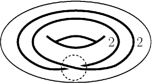
Figure 10.

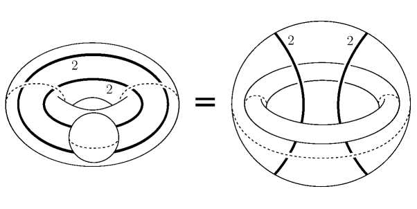
Figure 11. $C_{1}$

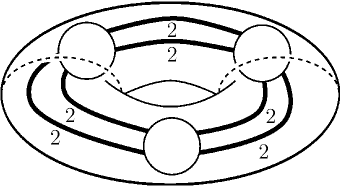
Figure 12. $C_{m}$, $m=3$

A connected component $Z$ of $X_{4}-\operatorname{int}({\mathcal{O}}^{2-stratum})$ can be described by a graph, i.e. a one-dimensional CW-complex, of degree $2$. Its vertices correspond to copies of

• A connected component of ${\mathcal{O}}^{0-stratum}_{Sph}$ with boundary $S^{2}$ or $S^{2}(k,k)$,

• A connected component of ${\mathcal{O}}^{0-stratum}_{Euc}$ with boundary $S^{2}(2,2,2,2)$, or

• $I\times S^{2}(2,2,2,2)$.

Each edge corresponds to a copy of

• $I\times D^{2}$,

• $I\times D^{2}(k)$ or

• $I\times D^{2}(2,2)$.

If a vertex is of type $I\times S^{2}(2,2,2,2)$ then the edge orbifolds only intersect the vertex orbifold on a single one of its two boundary components. Note that $|Z|$ is a solid torus with a certain number of balls removed.

A connected component of ${\mathcal{O}}^{0-stratum}_{Sph}$ is diffeomorphic to $D^{3}$, $D^{3}(k,k)$, $D^{3}(2,2,k)$, $I\times_{{\mathbb{Z}}_{2}}S^{2}$, or $I\times_{{\mathbb{Z}}_{2}}S^{2}(2,2,k)$. Now $I\times_{{\mathbb{Z}}_{2}}S^{2}$ is diffeomorphic to ${\mathbb{R}}P^{3}\#D^{3}$, $I\times_{{\mathbb{Z}}_{2}}S^{2}(k,k)$ is diffeomorphic to $(S^{3}(k,k)//{\mathbb{Z}}_{2})\#_{S^{2}(k,k)}D^{3}(k,k)$ and $I\times_{{\mathbb{Z}}_{2}}S^{2}(2,2,k)$ is diffeomorphic to $(S^{3}(2,2,k)//{\mathbb{Z}}_{2})\#_{S^{2}(2,2,k)}D^{3}(2,2,k)$, where ${\mathbb{Z}}_{2}$ acts by the antipodal action. Hence we can reduce to the case when each connected component of ${\mathcal{O}}^{0-stratum}_{Sph}$ is diffeomorphic to $D^{3}$, $D^{3}(k,k)$ or $D^{3}(2,2,k)$, modulo performing connected sums with the Seifert orbifolds ${\mathbb{R}}P^{3}$, $S^{3}(k,k)//{\mathbb{Z}}_{2}$ and $S^{3}(2,2,k)//{\mathbb{Z}}_{2}$.

Any connected component of ${\mathcal{O}}^{0-stratum}_{Euc}$ with boundary $S^{2}(2,2,2,2)$ can be written as the gluing of a weak graph orbifold with $I\times S^{2}(2,2,2,2)$. Hence we may assume that there are no vertices corresponding to connected components of ${\mathcal{O}}^{0-stratum}_{Euc}$ with boundary $S^{2}(2,2,2,2)$.

Suppose that there are no edges of type $I\times D^{2}(2,2)$. Then $Z$ is $I\times D^{2}$ or $I\times D^{2}(k)$, which is a weak graph orbifold.

Now suppose that there is an edge of type $I\times D^{2}(2,2)$. We build up a skeleton for $Z$. First, the orbifold corresponding to a graph with a single vertex of type $I\times S^{2}(2,2,2,2)$, and a single edge of type $I\times D^{2}(2,2)$, can be identified as the Seifert orbifold $C_{1}=S^{1}\times_{{\mathbb{Z}}_{2}}(S^{2}-3B^{2})$ of before. Let $C_{m}$ be the orbifold corresponding to a graph with $m$ vertices of type $I\times S^{2}(2,2,2,2)$ and $m$ edges of type $I\times D^{2}(2,2)$. See Figure 12. Then $C_{m}$ is an $m$-fold cover of $C_{1}$ and is also a Seifert orbifold.

Returning to the orbifold $Z$, there is some $m$ so that $Z$ is diffeomorphic to the result of starting with $C_{m}$ and gluing some $S^{1}\times_{{\mathbb{Z}}_{2}}D^{2}(k_{i})$’s onto some of the boundary $S^{2}(2,2,2,2)$’s, where $k_{i}\geq 1$. See Figure 13 for an illustrated example.

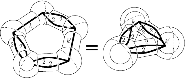
Figure 13.

Thus $Z$ is a weak graph orbifold.

As $X_{3}$ is the result of gluing $Z$ to a circle bundle over a surface, $X_{3}$ is a weak graph orbifold. Along with Proposition A.12, this proves the proposition. ∎

Proposition 9.7.

Let $c_{3}$ be the volume of the unit ball in ${\mathbb{R}}^{3}$, let $K\geq 10$ be a fixed integer and let $N$ be a positive integer. Fix a function $A:(0,\infty)\rightarrow(0,\infty)$. Then there is a $w_{0}\in(0,c_{3}/N)$ such that the following holds.

Suppose that $({\mathcal{O}},g)$ is a compact connected orientable Riemannian $3$-orbifold with boundary. Assume in addition that

1. $|G_{p}|\leq N$.

2. The diameters of the connected components of $\partial{\mathcal{O}}$ are bounded above by $w_{0}$.

3. For each component $X$ of $\partial{\mathcal{O}}$, there is a hyperbolic orbifold cusp ${\mathcal{H}}_{X}$ with boundary $\partial{\mathcal{H}}_{X}$, along with a $C^{K+1}$-embedding of pairs $e\>:\>(N_{100}(\partial{\mathcal{H}}_{X}),\partial{\mathcal{H}}_{X})\rightarrow({\mathcal{O}},X)$ which is $w_{0}$-close to an isometry.

4. For every $p\in|{\mathcal{O}}|$ with $d(p,\partial{\mathcal{O}})\geq 10$, we have, $\operatorname{vol}(B(p,R_{p}))\leq w_{0}R_{p}^{3}$.

5. For every $p\in|{\mathcal{O}}|$, $w^{\prime}\in[w_{0},c_{3}/N)$, $k\in[0,K]$ and $r\leq R_{p}$ such that $\operatorname{vol}(B(p,r))\geq w^{\prime}r^{3}$, the inequality

   (9.8) $$|\nabla^{k}\operatorname{Rm}|\leq A(w^{\prime})r^{-(k+2)}$$

   holds in the ball $B(p,r)$.

Then ${\mathcal{O}}$ is diffeomorphic to

• The result of performing $0$-surgeries on a strong graph orbifold,

• A closed isometric quotient of $S^{3}$ or $T^{3}$,

• $I\times S^{2}(2,3,6)$, $I\times S^{2}(2,4,4)$ or $I\times S^{2}(3,3,3)$, or

• $I\times_{{\mathbb{Z}}_{2}}S^{2}(2,3,6)$, $I\times_{{\mathbb{Z}}_{2}}S^{2}(2,4,4)$ or $I\times_{{\mathbb{Z}}_{2}}S^{2}(3,3,3)$.

Proof.

We follow the method of proof of [38, Section 16]. The effective difference from the proof of Proposition 9.1 is that we have additional components of ${\mathcal{O}}^{0-stratum}$, which are diffeomorphic to $I\times(T^{2}//\Gamma)$. If such a component is diffeomorphic to $I\times T^{2}$ or $I\times S^{2}(2,2,2,2)$ then we can incorporate it into the weak graph orbifold structure. The other cases give rise to the additional possibilities listed in the conclusion of the proposition. ∎

10. Incompressibility of cuspidal cross-sections and proof of Theorem 1.1

In this section we complete the proof of Theorem 1.1.

With reference to Proposition 8.9, given a sequence $t^{\alpha}\rightarrow\infty$, let $Y^{\alpha}$ be the truncation of $\coprod_{i=1}^{N}H_{i}$ obtained by removing horoballs at distance approximately $\frac{1}{2\beta(t^{\alpha})}$ from the basepoints $x_{i}$. Put ${\mathcal{O}}^{\alpha}={\mathcal{O}}_{t^{\alpha}}-f_{t^{\alpha}}(Y^{\alpha})$.

Proposition 10.1.

For large $\alpha$, the orbifold ${\mathcal{O}}^{\alpha}$ satisfies the hypotheses of Proposition 9.7.

Proof.

The proof is similar to that of [39, Theorem 17.3]. ∎

So far we know that if $\alpha$ is large then the $3$-orbifold ${\mathcal{O}}_{t^{\alpha}}$ has a (possibly empty) hyperbolic piece whose complement satisfies the conclusion of Proposition 9.7. In this section we show that there is such a decomposition of ${\mathcal{O}}_{t^{\alpha}}$ so that the hyperbolic cusps, if any, are incompressible in ${\mathcal{O}}_{t^{\alpha}}$.

The corresponding manifold result was proved by Hamilton in [34] using minimal disks. He used results of Meeks-Yau [43] to find embedded minimal disks with boundary on an appropriate cross-section of the cusp. The Meeks-Yau proof in turn used a tower construction [44] similar to that used in the proof of Dehn’s Lemma in $3$-manifold topology. It is not clear to us whether this line of proof extends to three-dimensional orbifolds, or whether there are other methods using minimal disks which do extend. To circumvent these issues, we use an alternative incompressibility argument due to Perelman [51, Section 8.2] that exploits certain quantities which change monotonically under the Ricci flow. Perelman’s monotonic quantity involved the smallest eigenvalue of a certain Schrödinger-type operator. We will instead use a variation of Perelman’s argument involving the minimal scalar curvature, following [38, Section 93.4].

Before proceeding, we need two lemmas:

Lemma 10.2.

Suppose $\epsilon>0$, and ${\mathcal{O}}^{\prime}$ is a Riemannian $3$-orbifold with scalar curvature $\geq-\frac{3}{2}$. Then any orbifold ${\mathcal{O}}$ obtained from ${\mathcal{O}}^{\prime}$ by $0$-surgeries admits a Riemannian metric with scalar curvature $\geq-\frac{3}{2}$, such that $\operatorname{vol}({\mathcal{O}})<\operatorname{vol}({\mathcal{O}}^{\prime})+\epsilon$.

Proof.

If a $0$-surgery adds a neck $(S^{2}//\Gamma)\times I$ then we can put a metric on the neck which is an isometric quotient of a slight perturbation of the doubled Schwarzschild metric [2, (1.23)] on $S^{2}\times I$. Hence we can perform the $0$-surgery so that the scalar curvature is bounded below by $-\frac{3}{2}+\frac{\epsilon}{10}$ and the volume increases by at most $\frac{\epsilon}{10}$; see [2, p. 155] and [52] for the analogous result in the manifold case. The lemma now follows from an overall rescaling to make $R\>\geq\>-\>\frac{3}{2}$. ∎

Lemma 10.3.

Suppose that ${\mathcal{O}}$ is a strong graph orbifold with boundary components $C_{1},\ldots,C_{k}$. Let $H_{1},\ldots,H_{k}$ be truncated hyperbolic cusps, where $\partial H_{i}$ is diffeomorphic to $C_{i}$ for all $i\in\{1,\ldots,k\}$. Then for all $\epsilon>0$, there is a metric on ${\mathcal{O}}$ with scalar curvature $\geq-\frac{3}{2}$ such that $\operatorname{vol}({\mathcal{O}})<\epsilon$, and $C_{i}$ has a collar which is isometric to one side of a collar neighborhood of a cuspical $2$-orbifold in $H_{i}$.

Proof.

We first prove the case when ${\mathcal{O}}$ is a closed strong graph manifold. The strong graph manifold structure gives a graph whose vertices $\{v_{a}\}$ correspond to the Seifert blocks and whose edges $\{e_{b}\}$ correspond to $2$-tori. For each vertex $v_{a}$, let $M_{a}$ be the corresponding Seifert block. We give it a Riemannian metric $g_{a}$ which is invariant under the local $S^{1}$-actions and with the property that the quotient metric on the orbifold base is a product near its boundary. Then $g_{a}$ has a product structure near $\partial M_{a}$. Given $\delta>0$, we uniformly shrink the Riemannian metric on $g_{a}$ by $\delta$ in the fiber directions. As $\delta\rightarrow 0$, the volume of $M_{a}$ goes to zero while the curvature stays bounded.

Let $T^{2}_{b}$ be the torus corresponding to the edge $e_{b}$. There are associated toral boundary components $\{B_{1},B_{2}\}$ of Seifert blocks. Given $\delta>0$ and $i\in\{1,2\}$, consider the warped product metric $ds^{2}+e^{-2s}g_{B_{i}}$ on a product manifold $P_{\delta,i}=[0,L_{\delta,i}]\times B_{i}$. We attach this at $B_{i}$ to obtain a $C^{0}$-metric, which we will smooth later. The sectional curvatures of $P_{\delta,i}$ are $-1$ and the volume of $P_{\delta,i}$ is bounded above by the area of $B_{i}$. We choose $L_{\delta,i}$ so that the areas of the cross-sections $\{L_{\delta,1}\}\times B_{1}$ and $\{L_{\delta,2}\}\times B_{2}$ are both equal to some number $A$. Finally, consider ${\mathbb{R}}^{3}$ with the $\operatorname{Sol}$-invariant metric $e^{-2z}dx^{2}+e^{2z}dy^{2}+dz^{2}$. Let $\Gamma$ be a ${\mathbb{Z}}^{2}$-subgroup of the normal ${\mathbb{R}}^{2}$-subgroup of $\operatorname{Sol}$. Note that the curvature of ${\mathbb{R}}^{3}/\Gamma$ is independent of $\Gamma$. The $z$-coordinate gives a fibering $z\>:\>{\mathbb{R}}^{3}/\Gamma\rightarrow{\mathbb{R}}$ with $T^{2}$-fibers. We can choose $\Gamma=\Gamma_{\delta}$ and an interval $[c_{1},c_{2}]\subset{\mathbb{R}}$ so that $z^{-1}(c_{1})$ is isometric to $\{L_{\delta,1}\}\times B_{1}$ and $z^{-1}(c_{2})$ is isometric to $\{L_{\delta,2}\}\times B_{2}$. Note that $[c_{1},c_{2}]$ can be taken independent of $A$. We attach $z^{-1}([c_{1},c_{2}])$ to the previously described truncated cusps, at the boundary components $\{L_{\delta,1}\}\times B_{1}$ and $\{L_{\delta,2}\}\times B_{2}$. See Figure 14.

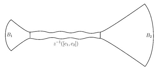
Figure 14.

Taking $A$ sufficiently small we can ensure that

(10.4) $$\operatorname{vol}(P_{\delta,1})+\operatorname{vol}(P_{\delta,2})+\operatorname{vol}(z^{-1}([c_{1},c_{2}]))<\operatorname{area}(B_{1})+\operatorname{area}(B_{2})+\delta.$$

We repeat this process for all of the tori $\{T^{2}_{b}\}$, to obtain a piecewise-smooth $C^{0}$-metric $g_{\delta}$ on ${\mathcal{O}}$.

As $\delta\rightarrow 0$, the sectional curvature stays uniformly bounded on the smooth pieces. Furthermore, the volume of $({\mathcal{O}},g_{\delta})$ goes to zero. By slightly smoothing $g_{\delta}$ and performing an overall rescaling to ensure that the scalar curvature is bounded below by $-\>\frac{3}{2}$, if $\delta$ is sufficiently small then we can ensure that $\operatorname{vol}({\mathcal{O}},g_{\delta})<\epsilon$. This proves the lemma when ${\mathcal{O}}$ is a closed strong graph manifold.

If ${\mathcal{O}}$ is a strong graph manifold but has nonempty boundary components, as in the hypotheses of the lemma, then we treat each boundary component $C_{i}$ analogously to a factor $B_{1}$ in the preceding construction. That is, given parameters $0<c_{1,C_{i}}<c_{2,C_{i}}$, we start by putting a truncated hyperbolic metric $ds^{2}+e^{-2s}g_{\partial H_{i}}$ on $\left[c_{1,C_{i}},c_{2,C_{i}}\right]\times C_{i}$. This will be the metric on the collar neighborhood of $C_{i}$, where $\{c_{1,C_{i}}\}\times C_{i}$ will end up becoming a boundary component of ${\mathcal{O}}$. We take $c_{2,C_{i}}$ so that the area of $\{c_{2,C_{i}}\}\times C_{i}$ matches the area of a relevant cross-section of the truncated cusp extending from a boundary component $B_{2,i}$ of a Seifert block. We then construct a metric $g_{\delta}$ on ${\mathcal{O}}$ as before. If we additionally take the parameters $\{c_{1,C_{i}}\}$ sufficiently large then we can ensure that $\operatorname{vol}({\mathcal{O}},g_{\delta})<\epsilon$.

Finally, if ${\mathcal{O}}$ is a strong graph orbifold then we can go through the same steps. The only additional point is to show that elements of the (orientation-preserving) mapping class group of an oriented Euclidean $2$-orbifold $T^{2}//\Gamma$ are represented by affine diffeomorphisms, in order to apply the preceding construction using the $\operatorname{Sol}$ geometry. To see this fact, if $\Gamma$ is trivial then the mapping class group of $T^{2}$ is isomorphic to $\operatorname{SL}(2,{\mathbb{Z}})$ and the claim is clear. To handle the case when $T^{2}//\Gamma$ is a sphere with three singular points, we use the fact that the mapping class group of a sphere with three marked points is isomorphic to the permutation group of the three points [25, Proposition 2.3]. The mapping class group of the orbifold $T^{2}//\Gamma$ will then be the subgroup of the permutation group that preserves the labels. If $T^{2}//\Gamma$ is $S^{2}(2,3,6)$ then its mapping class group is trivial. If $T^{2}//\Gamma$ is $S^{2}(2,4,4)$ then its mapping class group is isomorphic to ${\mathbb{Z}}_{2}$. Picturing $S^{2}(2,4,4)$ as two right triangles glued together, the nontrivial mapping class group element is represented by the affine diffeomorphism which is a flip around the “$2$” vertex that interchanges the two triangles. If $T^{2}//\Gamma$ is $S^{2}(3,3,3)$ then its mapping class group is isomorphic to $S_{3}$. Picturing $S^{2}(3,3,3)$ as two equilateral triangles glued together, the nontrivial mapping class group elements are represented by affine diffeomorphisms as rotations and flips. Finally, if $T^{2}//\Gamma$ is $S^{2}(2,2,2,2)$ then its mapping class group is isomorphic to $\operatorname{PSL}(2,{\mathbb{Z}})\ltimes({\mathbb{Z}}/2{\mathbb{Z}}\times{\mathbb{Z}}/2{\mathbb{Z}})$ [25, Proposition 2.7]. These all lift to ${\mathbb{Z}}_{2}$-equivariant affine diffeomorphisms of $T^{2}$. Elements of $\operatorname{PSL}(2,{\mathbb{Z}})$ are represented by linear actions of $\operatorname{SL}(2,{\mathbb{Z}})$ on $T^{2}$. Generators of ${\mathbb{Z}}/2{\mathbb{Z}}\times{\mathbb{Z}}/2{\mathbb{Z}}$ are represented by rotations of the $S^{1}$-factors in $T^{2}=S^{1}\times S^{1}$ by $\pi$. ∎

Let ${\mathcal{O}}$ be a closed connected orientable three-dimensional orbifold. If ${\mathcal{O}}$ admits a metric of positive scalar curvature then by finite extinction time, ${\mathcal{O}}$ is diffeomorphic to the result of performing $0$-surgeries on a disjoint collection of isometric quotients of $S^{3}$ and $S^{1}\times S^{2}$.

Suppose that ${\mathcal{O}}$ does not admit a metric of positive scalar curvature. Put

(10.5) $$\sigma({\mathcal{O}})=\sup_{g}R_{\min}(g)V(g)^{\frac{2}{3}}.$$

Then $\sigma({\mathcal{O}})\leq 0$.

Suppose that we have a given representation of ${\mathcal{O}}$ as the result of performing $0$-surgeries on the disjoint union of an orbifold ${\mathcal{O}}^{\prime}$ and isometric quotients of $S^{3}$ and $S^{1}\times S^{2}$, and that there exists a (possibly empty, possibly disconnected) finite-volume complete hyperbolic orbifold $N$ which can be embedded in ${\mathcal{O}}^{\prime}$ so that the connected components of the complement (if nonempty) satisfy the conclusion of Proposition 9.7. Let $V_{hyp}$ denote the hyperbolic volume of $N$. We do not assume that the cusps of $N$ are incompressible in ${\mathcal{O}}^{\prime}$.

Let $\widehat{V}$ denote the minimum of $V_{hyp}$ over all such decompositions of ${\mathcal{O}}$. (As the set of volumes of complete finite-volume three-dimensional hyperbolic orbifolds is well-ordered, there is a minimum. If there is a decomposition with $N=\emptyset$ then $V_{hyp}=0$.)

Lemma 10.6.

(10.7) $$\sigma({\mathcal{O}})=-\frac{3}{2}\widehat{V}^{\frac{2}{3}}.$$

Proof.

Using Lemmas 7.28, 10.2 and 10.3, the proof is similar to that of [38, Proposition 93.10]. ∎

Proposition 10.8.

Let $N$ be a hyperbolic orbifold as above for which $\operatorname{vol}(N)=\widehat{V}$. Then the cuspidal cross-sections of $N$ are incompressible in ${\mathcal{O}}^{\prime}$.

Proof.

As in [38, Section 93], it suffices to show that if a cuspidal cross-section of $N$ is compressible in ${\mathcal{O}}^{\prime}$ then there is a metric $g$ on ${\mathcal{O}}$ with $R(g)\geq-\frac{3}{2}$ and $\operatorname{vol}({\mathcal{O}},g)<\operatorname{vol}(N)$.

Put $Y={\mathcal{O}}^{\prime}-N$. Suppose that some connected component $C_{0}$ of $\partial Y$ is compressible, with compressing discal $2$-orbifold $Z\subset{\mathcal{O}}^{\prime}$. We can make $Z$ transverse to $\partial Y$ and then count the number of connected components of the intersection $Z\cap\partial Y$. Minimizing this number among all such compressing disks for all compressible components of $\partial Y$, we may assume – after possibly replacing $C_{0}$ with a different component of $\partial Y$ – that $Z$ intersects $\partial Y$ only along $\partial Z$.

By assumption, the components of $Y$ satisfy the conclusion of Proposition 9.7. Hence $Y$ has a decomposition into connected components $Y=Y_{0}\sqcup\ldots\sqcup Y_{n}$, where $Y_{0}$ is the component containing $C_{0}$, and $Y_{0}$ arises from a strong graph orbifold by $0$-surgeries, as otherwise there would not be a compressing discal orbifold. By Lemma A.16, $Y_{0}$ comes from a disjoint union $A\sqcup B$ via $0$-surgeries, where $A$ is one of the four solid-toric possibilities of that Lemma, and $B$ is a strong graph orbifold. By Lemmas 10.2 and 10.3, we may assume without loss of generality that $B=\emptyset$.

To construct the desired metric on ${\mathcal{O}}^{\prime}$, we proceed as follows. Let $H_{0},\ldots,H_{n}$ be the cusps of the hyperbolic orbifold $N$, where $H_{0}$ corresponds to the component $C_{0}$ of $Y$. We first truncate $N$ along totally umbilic cuspical $2$-orbifolds $C_{0},\ldots,C_{n}$. Pick $\epsilon>0$. For each $i\geq 1$ such that the component $Y_{i}$ comes from $0$-surgeries on a strong graph orbifold, we use Lemmas 10.2 and 10.3 to find a metric with $R\geq-\frac{3}{2}$ on $Y_{i}$, which glues isometrically along the corresponding cusps in $C_{1}\sqcup\ldots\sqcup C_{n}$, and which can be arranged to have volume $<\epsilon$ by taking the $C_{i}$’s to be deep in their respective cusps. For the components $Y_{i}$, $i\geq 1$, which do not come from a strong graph orbifold via $0$-surgery, we may also find metrics with $R\geq-\frac{3}{2}$ and arbitrarily small volume, which glue isometrically onto the corresponding truncated cusps of $N$ (when they have nonempty boundary). Our final step will be to find a metric on $Y_{0}=A$ with $R\geq-\frac{3}{2}$ which glues isometrically to $C_{0}$, and has volume strictly smaller than the portion of the cusp $H_{0}$ cut off by $C_{0}$. Since $\epsilon$ is arbitrary, this will yield a contradiction.

Suppose first that $A$ is $S^{1}\times D^{2}$ or $S^{1}\times D^{2}(k)$. In the $S^{1}\times D^{2}$ case, after going far enough down the cusp, the desired metric $g$ on $S^{1}\times D^{2}$ is constructed in [2, Pf. of Theorem 2.9]. (The condition $f_{2}(0)=a>0$ in [2, (2.47)] should be changed to $f_{2}(0)>0$.) In the $S^{1}\times D^{2}(k)$-case, [2, (2.46)] gets changed to $f_{1}^{\prime}(0)(1-a^{2})^{1/2}=1/k$. One can then make the appropriate modifications to [2, (2.54)-(2.56)] to construct the desired metric $g$ on $S^{1}\times D^{2}(k)$.

If $A$ is $S^{1}\times_{{\mathbb{Z}}_{2}}D^{2}$ or $S^{1}\times_{{\mathbb{Z}}_{2}}D^{2}(k)$ we can perform the construction of the previous paragraph equivariantly with respect to the ${\mathbb{Z}}_{2}$-action, to form the desired metric on $S^{1}\times_{{\mathbb{Z}}_{2}}D^{2}$ (or $S^{1}\times_{{\mathbb{Z}}_{2}}D^{2}(k)$). ∎

Proof of Theorem 1.1 : As mentioned before, if ${\mathcal{O}}$ admits a metric of positive scalar curvature then ${\mathcal{O}}$ is diffeomorphic to the result of performing $0$-surgeries on a disjoint collection of isometric quotients of $S^{3}$ and $S^{1}\times S^{2}$, so the theorem is true in that case. If ${\mathcal{O}}$ does not admit a metric of positive scalar curvature then by Proposition 10.8,

1. ${\mathcal{O}}$ is the result of performing $0$-surgeries on an orbifold ${\mathcal{O}}^{\prime}$ and a disjoint collection of isometric quotients of $S^{3}$ and $S^{1}\times S^{2}$, such that

2. There is a finite-volume complete hyperbolic orbifold $N$ which can be embedded in ${\mathcal{O}}^{\prime}$ so that each connected component ${\mathcal{P}}$ of the complement (if nonempty) has a metric completion $\overline{\mathcal{P}}$ which satisfies the conclusion of Proposition 9.7, and

3. The cuspidal cross-sections of $N$ are incompressible in ${\mathcal{O}}^{\prime}$.

Referring to Proposition 9.7, if $\overline{\mathcal{P}}$ is an isometric quotient of $S^{3}$ or $T^{3}$ then it already has a geometric structure. If $\overline{\mathcal{P}}$ is $I\times S^{2}(p,q,r)$ with $\frac{1}{p}+\frac{1}{q}+\frac{1}{r}=1$ then we can remove it without losing any information. If $\overline{\mathcal{P}}$ is $I\times_{{\mathbb{Z}}_{2}}S^{2}(p,q,r)$ with $\frac{1}{p}+\frac{1}{q}+\frac{1}{r}=1$ then ${\mathcal{P}}$ has a Euclidean structure.

Finally, suppose that $\overline{\mathcal{P}}$ is the result of performing $0$-surgeries on a collection of strong graph orbifolds in the sense of Definition A.8. A Seifert-fibered $3$-orbifold with no bad $2$-dimensional suborbifolds is geometric in the sense of Thurston [5, Proposition 2.13]. This completes the proof of Theorem 1.1.

Remark 10.9.

The geometric decomposition of ${\mathcal{O}}$ that we have produced, using strong graph orbifolds, will not be minimal if ${\mathcal{O}}$ has $\operatorname{Sol}$ geometry. In such a case, ${\mathcal{O}}$ fibers over a $1$-dimensional orbifold. Cutting along a fiber and taking the metric completion gives a product orbifold, which is a graph orbifold. Of course, the minimal geometric decomposition of ${\mathcal{O}}$ would leave it with its $\operatorname{Sol}$ structure.

Remark 10.10.

Theorem 1.1 implies that ${\mathcal{O}}$ is very good, i.e. the quotient of a manifold by a finite group action [4, Corollary 1.3]. Hence one could obtain the geometric decomposition of ${\mathcal{O}}$ by running Perelman’s proof equivariantly, as is done in detail for elliptic and hyperbolic manifolds in [21]. However, one cannot prove the geometrization of orbifolds this way, as the reasoning would be circular; one only knows that ${\mathcal{O}}$ is very good after proving Theorem 1.1.

Appendix A Weak and strong graph orbifolds

In this appendix we provide proofs of some needed facts about graph orbifolds. We show that a weak graph orbifold is the result of performing $0$-surgeries on a strong graph orbifold. (Since we don’t require strong graph orbifolds to be connected, we need only one.) A similar result appears in [24, Section 2.4].

In order to clarify the arguments, we prove the corresponding manifold results before proving the orbifold results.

Definition A.1.

A weak graph manifold is a compact orientable $3$-manifold $M$ for which there is a collection $\{T_{i}\}$ of disjoint embedded tori in $\operatorname{int}(M)$ so that after splitting $M$ open along $\{T_{i}\}$, the result has connected components that are Seifert-fibered $3$-manifolds (possibly with boundary).

We do not assume that $M$ is connected. Here “splitting $M$ open along $\{T_{i}\}$” means taking the metric completion of $M-\bigcup_{i}T_{i}$ with respect to an arbitrary Riemannian metric on $M$.

Remark A.2.

In the definition of a weak graph manifold, we could have instead required that the connected components of the metric completion of $M-\bigcup_{i}T_{i}$ are circle bundles over surfaces. This would give an equivalent notion, since any Seifert-fibered $3$-manifold can be cut along tori into circle bundles over surfaces.

For notation, we will write $S^{2}-kB^{2}$ for the complement of $k$ disjoint separated open $2$-balls in $S^{2}$.

Definition A.3.

A strong graph manifold is a compact orientable $3$-manifold $M$ for which there is a collection $\{T_{i}\}$ of disjoint embedded tori in $\operatorname{int}(M)$ such that

1. After splitting $M$ open along $\{T_{i}\}$, the result has connected components that are Seifert manifolds (possibly with boundary).

2. For any $T_{i}$, the two circle fibrations on $T_{i}$ coming from the adjacent Seifert bundles are not isotopic.

3. Each $T_{i}$ is incompressible in $M$.

A.1. Weak graph manifolds are connected sums of strong graph manifolds

The next lemma states if we glue two solid tori (respecting orientations) then the result is a Seifert manifold. The lemma itself is trivial, since we know that the manifold is $S^{1}\times S^{2}$, $S^{3}$ or a lens space, each of which is a Seifert manifold. However, we give a proof of the lemma which will be useful in the orbifold case.

Lemma A.4.

Let $U$ and $V$ be two oriented solid tori. Let $\phi:\partial U\rightarrow\partial V$ be an orientation-reversing diffeomorphism. Then $U\cup_{\phi}V$ admits a Seifert fibration.

Proof.

We first note that the circle fiberings of $T^{2}$ are classified (up to isotopy) by the image of the fiber in $(\operatorname{H}^{1}(T^{2};{\mathbb{Z}})-\{0\})/\{\pm 1\}\simeq({\mathbb{Z}}^{2}-\{0\})/\{\pm 1\}$. There is one circle fibering of $\partial U$ (up to isotopy) whose fibers bound compressing disks in $U$. Any other circle fibering of $\partial U$ is the boundary fibration of a Seifert fibration of $U$. Hence we can choose a circle fibering ${\mathcal{F}}$ of $\partial U$ so that ${\mathcal{F}}$ is the boundary fibration of a Seifert fibration of $U$, and $\phi_{*}{\mathcal{F}}$ is the boundary fibration of a Seifert fibration of $V$. The ensuing Seifert fibrations of $U$ and $V$ join together to give a Seifert fibration of $U\cup_{\phi}V$. ∎

Proposition A.5.

If a connected strong graph manifold contains an essential embedded $2$-sphere then it is diffeomorphic to $S^{1}\times S^{2}$ or ${\mathbb{R}}P^{3}\#{\mathbb{R}}P^{3}$.

Proof.

Suppose that a connected strong graph manifold $M$ contains an essential embedded $2$-sphere $S$. We can assume that $S$ is transverse to $\bigcup_{i}T_{i}$. We choose $S$ among all such essential embedded $2$-spheres so that the number of connected components of $S\cap\bigcup_{i}T_{i}$ is as small as possible.

If $S\cap\bigcup_{i}T_{i}=\emptyset$ then $S$ is an essential $2$-sphere in one of the Seifert components.

If $S\cap\bigcup_{i}T_{i}\neq\emptyset$, let $C$ be an innermost circle in $S\cap\bigcup_{i}T_{i}$. Then $C\subset T_{k}$ for some $k$ and $C=\partial D$ for some $2$-disk $D$ embedded in a Seifert component $U$ with $T_{k}\subset\partial U$. As $T_{k}$ is incompressible, $C=\partial D^{\prime}$ for some $2$-disk $D^{\prime}\subset T_{k}$. If $D\cup D^{\prime}$ bounds a $3$-ball in $U$ then we can isotope $S$ to remove the intersection with $T_{k}$, which contradicts the choice of $S$. Thus $D\cup D^{\prime}$ is an essential $2$-sphere in $U$.

In any case, we found an essential $2$-sphere in one of the Seifert pieces. It follows that the Seifert piece, and hence all of $M$, is diffeomorphic to $S^{1}\times S^{2}$ or ${\mathbb{R}}P^{3}\#{\mathbb{R}}P^{3}$ [55, p. 432]. ∎

Proposition A.6.

A weak graph manifold is the result of performing $0$-surgeries on a strong graph manifold.

Proof.

Suppose that Proposition A.6 fails. Let $n$ be the minimal number of decomposing tori among weak graph manifolds which are counterexamples, and let $M$ be a counterexample with decomposing tori $\{T_{i}\}_{i=1}^{n}$.

We first look for a torus $T_{j}$ for which the two induced circle fibrations (coming from the adjacent Seifert bundles) are isotopic. If there is one then we extend the Seifert fibration over $T_{j}$. In this case, by removing $T_{j}$ from $\{T_{i}\}_{i=1}^{n}$, we get a weak graph decomposition of $M$ with $(n-1)$ tori, contradicting the definition of $n$.

Therefore there is no such torus. Since $M$ is a counterexample to Proposition A.6, there must be a torus in $\{T_{i}\}_{i=1}^{n}$ which is compressible. Let $D$ be a compressing disk, which we can assume to be transversal to $\bigcup_{i=1}^{n}T_{i}$. We choose such a compressing disk so that $D\cap\bigcup_{i=1}^{n}T_{i}$ has the smallest possible number of connected components. Let $C$ be an innermost circle in $D\cap\bigcup_{i=1}^{n}T_{i}$, say lying in $T_{k}$. Then $C$ bounds a disk $D^{\prime}$ in a Seifert bundle $V$ which has $T_{k}$ as a boundary component.

If $C$ also bounds a disk $D^{\prime\prime}\subset T_{k}$ then $D^{\prime}\cup D^{\prime\prime}$ is an embedded $2$-sphere $S$ in $V$. If $S$ is not essential in $V$ then we can isotope $D$ so that it does not intersect $T_{k}$, which contradicts the choice of $D$. So $S$ is essential in $V$. Then $V$ is diffeomorphic to $S^{1}\times S^{2}$ or ${\mathbb{R}}P^{3}\#{\mathbb{R}}P^{3}$, which contradicts the assumption that it has $T_{k}$ as a boundary component.

Thus we can assume that $D^{\prime}$ is a compressing disk for $V$, which is necessarily a solid torus [55, Corollary 3.3].

Let $U$ be the Seifert bundle on the other side of $T_{k}$ from $V$. Let $B$ be the orbifold base of $U$, with projection $\pi:U\rightarrow B$. There is a circle boundary component $R\subset\partial B$ so that $T_{k}=\pi^{-1}(R)$. That is, $V$ is glued to $U$ along $\pi^{-1}(R)$. Choose a $D^{2}$-fibration $\sigma:V\rightarrow R$ that extends $\pi:T_{k}\rightarrow R$.

If $C=\partial D^{\prime}\subset T_{k}$ is not isotopic to a fiber of $\pi\Big{|}_{T_{k}}$, let $u>0$ be their algebraic intersection number in $T_{k}$. Then $U\cup_{T_{k}}V$ has a Seifert fibration over $B\cup_{R}D^{2}(u)$. Removing $T_{k}$ from $\{T_{i}\}_{i=1}^{n}$, we again have a weak graph decomposition of $M$, now with $(n-1)$ tori, which is a contradiction.

Therefore $C=\partial D^{\prime}\subset T_{k}$ is isotopic to a fiber of $\pi\Big{|}_{T_{k}}$.

Step 1: If $B$ is diffeomorphic to $D^{2}$, $D^{2}(r)$ or $S^{1}\times I$ then put $M^{\prime}=M$ and $B^{\prime}=B$, and go to Step 2. Otherwise, let $\{\gamma_{j}\}_{j=1}^{J}$ be a maximal disjoint collection of smooth embedded arcs $\gamma_{j}:[0,1]\rightarrow B_{reg}$, with $\{\gamma_{j}(0),\gamma_{j}(1)\}\subset R$, which determine distinct nontrivial homotopy classes for the pair $(B_{reg},R)$. (Note that $\partial B\subset B_{reg}$.) If $B^{\prime}$ is the result of splitting $B$ open along $\{\gamma_{j}\}_{j=1}^{J}$, then the connected components of $B^{\prime}$ are diffeomorphic to $D^{2}$, $D^{2}(r)$ for some $r>1$, or $S^{1}\times I$. See Figure 15.

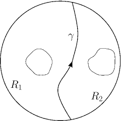
Figure 15.

Let $R^{\prime}$ be the result of splitting the $1$-manifold $R$ along the finite subset $\bigcup_{j=1}^{J}\{\gamma_{j}(0),\gamma_{j}(1)\}$.

Define a $2$-sphere $S^{2}_{j}\subset M$ by $S^{2}_{j}=\sigma^{-1}(\gamma_{j}(0))\cup_{\pi^{-1}(\gamma_{j}(0))}\pi^{-1}(\gamma_{j})\cup_{\pi^{-1}(\gamma_{j}(1))}\sigma^{-1}(\gamma_{j}(1))$. Let $Y$ be the result of splitting $M$ open along $\{S^{2}_{j}\}_{j=1}^{J}$. It has $2J$ spherical boundary components corresponding to the spherical cuts. We glue on $2J$ $3$-disks there, to obtain $M^{\prime}$. By construction, $M$ is the result of performing $J$ $0$-surgeries on $M^{\prime}$.

We claim that $M^{\prime}$ is a weak graph manifold. To see this, note that the union $W$ of the $D^{2}$-bundle over $R^{\prime}$ and the $2J$ 3-disks is a disjoint union of solid tori in $M^{\prime}$; see Figure 15. The metric completion of $M^{\prime}-W$ inherits a weak graph structure from $M$. This shows that $M^{\prime}$ is a weak graph manifold.

Step 2 : For each component $P$ of $B^{\prime}$ that is diffeomorphic to $D^{2}$ or $D^{2}(r)$, the corresponding component of $M^{\prime}$ is the result of gluing two solid tori: one being $\pi^{-1}(P)$ and the other one being a connected component of $W$. By Lemma A.4, this component of $M^{\prime}$ is Seifert-fibered and hence is a strong graph manifold. We discard all such components of $M^{\prime}$ and let $\widehat{M}$ denote what’s left.

A component $P$ of $B^{\prime}$ diffeomorphic to $S^{1}\times I$ has a boundary consisting of two circles $C_{1}$ and $C_{2}$, of which exactly one, say $C_{1}$, does not intersect $R$. In $\widehat{M}$, the preimage $\pi^{-1}(C_{1})$ is attached to the union of $\pi^{-1}(P)$ with a solid torus. This union is itself a solid torus.

In this way, we see that $\widehat{M}$ has a weak graph decomposition with $(n-1)$ tori, since $T_{k}$ has disappeared. Since $M$ was a counterexample to Proposition A.6, it follows that $\widehat{M}$ is also a counterexample. This contradicts the definition of $n$ and so proves the proposition. ∎

A.2. Weak graph orbifolds are connected sums of strong graph orbifolds

In this section we only consider $3$-dimensional orbifolds that do not admit embedded bad $2$-dimensional suborbifolds.

Definition A.7.

A weak graph orbifold is a compact orientable $3$-orbifold ${\mathcal{O}}$ for which there is a collection $\{E_{i}\}$ of disjoint embedded orientable Euclidean $2$-orbifolds in $\operatorname{int}({\mathcal{O}})$ so that after splitting ${\mathcal{O}}$ open along $\{E_{i}\}$, the result has connected components that are Seifert-fibered orbifolds (possibly with boundary).

Definition A.8.

A strong graph orbifold is a compact orientable $3$-orbifold ${\mathcal{O}}$ for which there is a collection $\{E_{i}\}$ of disjoint embedded orientable Euclidean $2$-orbifolds in $\operatorname{int}({\mathcal{O}})$ such that

1. After splitting ${\mathcal{O}}$ open along $\{E_{i}\}$, the result has connected components that are Seifert orbifolds (possibly with boundary).

2. For any $E_{i}$, the two circle fibrations on $E_{i}$ coming from the adjacent Seifert bundles are not isotopic.

3. Each $E_{i}$ is incompressible in ${\mathcal{O}}$.

From Subsection 2.4, each $E_{i}$ is diffeomorphic to $T^{2}$ or $S^{2}(2,2,2,2)$.

Lemma A.9.

Let $U$ and $V$ be two oriented solid-toric $3$-orbifolds with diffeomorphic boundaries. Let $\phi:\partial U\rightarrow\partial V$ be an orientation-reversing diffeomorphism. Then $U\cup_{\phi}V$ admits a Seifert orbifold structure.

Proof.

Suppose first that $\partial U$ is a $2$-torus. Then $U$ is diffeomorphic to $S^{1}\times D^{2}$ or $S^{1}\times D^{2}(k)$. The Seifert orbifold structures on $U$ are in one-to-one correspondence with the Seifert manifold structures on $|U|$ [7, p. 36-37]. There is one circle fibering of $\partial U$ (up to isotopy) whose fibers bound compressing discal $2$-orbifolds in $U$. Any other circle fibering of $\partial U$ is the boundary fibration of a Seifert fibration of $U$. As in the proof of Lemma A.4, we can choose a circle fibering ${\mathcal{F}}$ of $\partial U$ so that ${\mathcal{F}}$ is the boundary fibration of a Seifert fibration of $U$, and $\phi_{*}{\mathcal{F}}$ is the boundary fibration of a Seifert fibration of $V$. The ensuing Seifert fibrations of $U$ and $V$ join together to give a Seifert fibration of $U\cup_{\phi}V$.

Now suppose that $\partial U$ is diffeomorphic to $S^{2}(2,2,2,2)$. The orbifiberings of $S^{2}(2,2,2,2)$ with one-dimensional fiber are the ${\mathbb{Z}}_{2}$-quotients of ${\mathbb{Z}}_{2}$-invariant circle fiberings of $T^{2}$. In particular, there is an infinite number of such orbifiberings up to isotopy. (More concretely, given an orbifibering, there are two disjoint arc fibers connecting pairs of singular points. The complement of the two arcs in $|S^{2}(2,2,2,2)|$ is an open cylinder with an induced circle fibering. The isotopy class of the orbifibering is specified by the isotopy class of the two disjoint arcs.)

From [7, p. 38-39], the Seifert fibrations of $U$ are the ${\mathbb{Z}}_{2}$-quotients of ${\mathbb{Z}}_{2}$-invariant Seifert fibrations of its solid-toric double cover. It follows that there is one orbifibering of $\partial U$ (up to isotopy) whose fibers bound compressing discal $2$-orbifolds in $U$. Any other orbifibering of $\partial U$ is the boundary fibration of a Seifert fibration of $U$. Hence we can choose an orbifibering ${\mathcal{F}}$ of $\partial U$ so that ${\mathcal{F}}$ is the boundary fibration of a Seifert fibration of $U$, and $\phi_{*}{\mathcal{F}}$ is the boundary fibration of a Seifert fibration of $V$. The ensuing Seifert fibrations of $U$ and $V$ join together to give a Seifert fibration of $U\cup_{\phi}V$. ∎

Proposition A.10.

If a connected strong graph orbifold contains an essential embedded spherical $2$-orbifold then it is diffeomorphic to a finite isometric quotient of $S^{1}\times S^{2}$.

Proof.

Suppose that a connected strong graph orbifold ${\mathcal{O}}$ contains an essential embedded spherical $2$-orbifold $S$.

Lemma A.11.

After an isotopy of $S$, we can assume that $S\cap\bigcup_{i}E_{i}$ is a disjoint collection of closed curves in the regular part of $S$.

Proof.

If $E_{i}$ is diffeomorphic to $T^{2}$ then a neighborhood of $E_{i}$ lies in $|{\mathcal{O}}|_{reg}$ and after isotopy, $S\cap E_{i}$ is a disjoint collection of closed curves in the regular part of $S$. Suppose that $E_{i}$ is diffeomorphic to $S^{2}(2,2,2,2)$. A neighborhood of $E_{i}$ is diffeomorphic to $I\times E_{i}$. Suppose that $p\in S$ is a singular point of $E_{i}$. Then the local group of $p$ in $S$ must be ${\mathbb{Z}}_{2}$. After pushing a neighborhood of $p\in S$ slightly in the $I$-direction of $I\times E_{i}$, we can remove the intersection of $S$ with that particular singular point of $E_{i}$. In this way, we can arrange so that $S$ intersects $\bigcup_{i}E_{i}$ transversely, with the intersection lying in the regular part of $S$. ∎

We choose $S$ among all such essential embedded spherical $2$-orbifolds so that the number of connected components of $|S\cap\bigcup_{i}E_{i}|$ is as small as possible.

If $S\cap\bigcup_{i}E_{i}=\emptyset$ then $S$ is an essential embedded spherical $2$-orbifold in one of the Seifert pieces.

If $S\cap\bigcup_{i}E_{i}\neq\emptyset$, let $C\subset|S|$ be an innermost circle in $|S\cap\bigcup_{i}E_{i}|$. Then $C\subset|E_{k}|$ for some $k$, and $C=\partial D$ for some discal $2$-orbifold $D$ embedded in a Seifert component $U$ with $E_{k}\subset\partial U$. As $E_{k}$ is incompressible, $C=\partial D^{\prime}$ for some discal $2$-orbifold $D^{\prime}\subset E_{k}$. Then $D\cup D^{\prime}$ is an embedded $2$-orbifold with underlying space $S^{2}$ and at most two singular points. As ${\mathcal{O}}$ has no bad $2$-suborbifolds, $D\cup D^{\prime}$ must be diffeomorphic to $S^{2}(r,r)$ for some $r\geq 1$. If $D\cup D^{\prime}$ bounds some $D^{3}(r,r)$ in $U$ then we can isotope $S$ to remove the intersection with $E_{k}$, which contradicts the choice of $S$. Thus $D\cup D^{\prime}$ is an essential embedded spherical $2$-orbifold in $U$.

In any case, we found an essential embedded spherical $2$-orbifold in one of the Seifert pieces. Then the universal cover of the Seifert piece contains an essential embedded $S^{2}$. It follows that the universal cover of the Seifert piece is ${\mathbb{R}}\times S^{2}$ [5, Proposition 2.13]. The Seifert piece, and hence all of ${\mathcal{O}}$, must then be diffeomorphic to a finite isometric quotient of $S^{1}\times S^{2}$. ∎

Proposition A.12.

A weak graph orbifold is the result of performing $0$-surgeries on a strong graph orbifold.

Proof.

Suppose that Proposition A.12 fails. Let $n$ be the minimal number of decomposing Euclidean $2$-orbifolds among weak graph orbifolds which are counterexamples, and let ${\mathcal{O}}$ be a counterexample with decomposing Euclidean $2$-orbifolds $\{E_{i}\}_{i=1}^{n}$.

We first look for a $2$-orbifold $E_{j}$ for which the two induced circle fibrations (coming from the adjacent Seifert bundles) are isotopic, in the sense of [5, Chapter 2.5]. If there is one then we extend the Seifert fibration over $E_{j}$. In this case, by removing $E_{j}$ from $\{E_{i}\}$, we get a weak graph decomposition of ${\mathcal{O}}$ with $(n-1)$ Euclidean $2$-orbifolds, contradicting the definition of $n$.

Therefore there is no such Euclidean $2$-orbifold. Since ${\mathcal{O}}$ is a counterexample to Proposition A.12, there must be a Euclidean $2$-orbifold in $\{E_{i}\}$ which is compressible. Let $D$ be a compressing discal $2$-orbifold. As in Lemma A.11, we can assume that $D$ intersects $\bigcup_{i}E_{i}$ transversally, with the intersection lying in the regular part of $D$. We choose such a compressing discal $2$-orbifold so that $D\cap\bigcup_{i}E_{i}$ has the smallest possible number of connected components. Let $C$ be an innermost circle in $D\cap\bigcup_{i}E_{i}$, say lying in $|E_{k}|$. Then $C$ bounds a discal $2$-orbifold $D^{\prime}$ lying in a Seifert bundle $V$ which has $E_{k}$ as a boundary component.

If $C$ also bounds a discal $2$-orbifold $D^{\prime\prime}\subset E_{k}$ then $D^{\prime}\cup D^{\prime\prime}$ is an embedded $2$-orbifold $S$ in the Seifert bundle. As there are no bad $2$-orbifolds in ${\mathcal{O}}$, the suborbifold $S$ must be diffeomorphic to $S^{2}(r,r)$ for some $r\geq 1$. If $S$ is not essential in $V$ then it bounds a $D^{3}(r,r)$ in $V$ and we can isotope $D$ so that it does not intersect $E_{k}$, which contradicts the choice of $D$. So $S$ is essential in $V$. From Proposition A.10, the Seifert bundle $V$ is diffeomorphic to a finite isometric quotient of $S^{1}\times S^{2}$, which contradicts the assumption that it has $E_{k}$ as a boundary component.

Thus we can assume that $C$ bounds a compressing discal $2$-orbifold for $V$, which is necessarily a solid-toric orbifold diffeomorphic to $S^{1}\times D^{2}(r)$ or $S^{1}\times_{{\mathbb{Z}}_{2}}D^{2}(r)$ for some $r\geq 1$ [19, Lemma 2.47].

Let $U$ be the Seifert bundle on the other side of $E_{k}$ from $V$. Let $B$ be the orbifold base of $U$, with projection $\pi:U\rightarrow B$. There is a $1$-orbifold boundary component $R\subset\partial B$, diffeomorphic to $S^{1}$ or $S^{1}//{\mathbb{Z}}_{2}$, so that $E_{k}=\pi^{-1}(R)$. That is, $V$ is glued to $U$ along $\pi^{-1}(R)$. Choose a discal orbifibration $\sigma:V\rightarrow R$ that extends $\pi:E_{k}\rightarrow R$.

We refer to [5, Chapter 2.5] for a discussion of Dehn fillings, i.e. gluings of $V$ to $\pi^{-1}(R)$. If the meridian curve of $V$ is not isotopic to a fiber of $\pi\Big{|}_{E_{k}}$, let $u>0$ be the algebraic intersection number (computed using the maximal abelian subgroup of $\pi_{1}(E_{k})$). Then the gluing of $V$ to $U$, along $\pi^{-1}(R)$, has a Seifert fibration. Removing $E_{k}$ from $\{E_{i}\}$, we again have a weak graph orbifold decomposition of ${\mathcal{O}}$, now with $(n-1)$ Euclidean 2-orbifolds, which is a contradiction.

Therefore, the meridian curve of $V$ is isotopic to a fiber of $\pi\Big{|}_{E_{k}}$.

Step 1 : If one of the following possibilities holds then put ${\mathcal{O}}^{\prime}={\mathcal{O}}$ and $B^{\prime}=B$, and go to Step 2:

1. $B=D^{2}$.

2. $B=D^{2}(s)$ for some $s>1$.

3. $B=D^{2}//{\mathbb{Z}}_{2}$.

4. $B=D^{2}(s)//{\mathbb{Z}}_{2}$ for some $s>1$.

5. $B=S^{1}\times I$.

6. $B=(S^{1}//{\mathbb{Z}}_{2})\times I$.

Otherwise, we split $B$ open along a disjoint collection of smooth embedded arcs $\{\gamma_{j}\}_{j=1}^{J}\cup\{\gamma^{\prime}_{j^{\prime}}\}_{j^{\prime}=1}^{J^{\prime}}$ of the following type. A curve $\gamma_{j}:[0,1]\rightarrow B$ lies in $B_{reg}$ and has $|\gamma_{j}|(0),|\gamma_{j}|(1)\in\operatorname{int}(|R|)$. A curve $\gamma_{j^{\prime}}:[0,1]\rightarrow B$ has $|\gamma_{j^{\prime}}|(0)\in\operatorname{int}(|R|)$ and lies in $B_{reg}$, except for its endpoint $|\gamma_{j^{\prime}}|(1)$ which is in the interior of a reflector component of $\partial|B|$ but is not a corner reflector point. We can find a collection of such curves so that if $B^{\prime}$ is the result of splitting $B$ open along them, then each connected component of $B^{\prime}$ is of type (1)-(6) above. Put

(A.13) $$R^{\prime}=R-\bigcup_{j=1}^{J}\{|\gamma_{j}|(0),|\gamma_{j}|(1)\}-\bigcup_{j^{\prime}=1}^{J^{\prime}}\{|\gamma_{j^{\prime}}|(0)\}.$$

Associated to $\gamma_{j}$ is a spherical $2$-orbifold $X_{j}$, diffeomorphic to $S^{2}(r,r)$, given by

(A.14) $$X_{j}=\sigma^{-1}(\gamma_{j}(0))\cup_{\pi^{-1}(\gamma_{j}(0))}\pi^{-1}(\gamma_{j})\cup_{\pi^{-1}(\gamma_{j}(1))}\sigma^{-1}(\gamma_{j}(1)).$$

Associated to $\gamma^{\prime}_{j^{\prime}}$ is a spherical $2$-orbifold $X^{\prime}_{j^{\prime}}$, diffeomorphic to $S^{2}(2,2,r)$, given by

(A.15) $$X^{\prime}_{j^{\prime}}=\sigma^{-1}(\gamma_{j^{\prime}}(0))\cup_{\pi^{-1}(\gamma_{j^{\prime}}(0))}\pi^{-1}(\gamma_{j^{\prime}}).$$

Let $Y$ be the result of splitting ${\mathcal{O}}$ open along $\{X_{j}\}_{j=1}^{J}\cup\{X^{\prime}_{j^{\prime}}\}_{j^{\prime}=1}^{J^{\prime}}$. It has $2(J+J^{\prime})$ spherical boundary components corresponding to the spherical cuts. We glue on $2J$ copies of $D^{3}(r,r)$ and $2J^{\prime}$ copies of $D^{3}(2,2,r)$, to obtain ${\mathcal{O}}^{\prime}$. By construction, ${\mathcal{O}}$ is the result of performing $0$-surgeries on ${\mathcal{O}}^{\prime}$.

We claim that ${\mathcal{O}}^{\prime}$ is a weak graph orbifold. To see this, note that the union $W$ of $\sigma^{-1}(R^{\prime})$ and the $2(J+J^{\prime})$ discal $3$-orbifolds is a disjoint union of solid-toric $3$-orbifolds in ${\mathcal{O}}^{\prime}$. The metric completion of $|{\mathcal{O}}^{\prime}|-|W|$ in $|{\mathcal{O}}^{\prime}|$ inherits a weak graph orbifold structure from ${\mathcal{O}}$. This shows that ${\mathcal{O}}^{\prime}$ is a weak graph orbifold.

Step 2 : For each connected component of $B^{\prime}$ of type (1)-(4) above, the corresponding component of ${\mathcal{O}}^{\prime}$ is the result of gluing two solid-toric orbifolds: one being the Seifert orbifold over that component of $B^{\prime}$, and the other one being a connected component of $W$. By Lemma A.9, this component of ${\mathcal{O}}^{\prime}$ is Seifert-fibered and hence is a strong graph orbifold. We discard all such components of ${\mathcal{O}}^{\prime}$ and let $\widehat{{\mathcal{O}}}$ denote what’s left.

Turning to the remaining possibilities, an annular component $P$ of $B^{\prime}$ has a boundary consisting of two circles $C_{1}$ and $C_{2}$, of which exactly one, say $C_{1}$, does not intersect $R$. In $\widehat{{\mathcal{O}}}$, the preimage $\pi^{-1}(C_{1})$ is attached to the union of $\pi^{-1}(P)$ with a solid-toric orbifold diffeomorphic to $S^{1}\times D^{2}(r)$. This union is itself diffeomorphic to $S^{1}\times D^{2}(r)$, since $\pi^{-1}(P)$ is diffeomorphic to $S^{1}\times S^{1}\times I$.

Finally, if a component $P$ of $B^{\prime}$ is diffeomorphic to $(S^{1}//{\mathbb{Z}}_{2})\times I$ then $\partial|P|$ consists of a circle with two reflector components and two nonreflector components. Exactly one of the nonreflector components, say $C_{1}$, does not intersect $R$. In $\widehat{{\mathcal{O}}}$, the preimage $\pi^{-1}(C_{1})$ is attached to the union of $\pi^{-1}(P)$ with a solid-toric orbifold diffeomorphic to $S^{1}\times_{{\mathbb{Z}}_{2}}D^{2}(r)$. This union is itself diffeomorphic to $S^{1}\times_{{\mathbb{Z}}_{2}}D^{2}(r)$, since $\pi^{-1}(P)$ is diffeomorphic to $(S^{1}\times_{{\mathbb{Z}}_{2}}S^{1})\times I$.

In this way, we see that $\widehat{{\mathcal{O}}}$ has a weak graph orbifold decomposition with $(n-1)$ Euclidean $2$-orbifolds, since $E_{k}$ has disappeared. Since ${\mathcal{O}}$ was a counterexample to Proposition A.12, it follows that $\widehat{{\mathcal{O}}}$ is also a counterxample. This contradicts the definition of $n$ and so proves the proposition. ∎

A.3. Weak graph orbifolds with a compressible boundary component

Lemma A.16.

Suppose that ${\mathcal{O}}$ is a weak graph orbifold, and that $C\subset\partial{\mathcal{O}}$ is a compressible boundary component. Then ${\mathcal{O}}$ arises from $0$-surgery on a disjoint collection ${\mathcal{O}}_{0}\sqcup\ldots\sqcup{\mathcal{O}}_{n}$, where:

• ${\mathcal{O}}_{i}$ is a strong graph manifold for all $i$.

• $\partial{\mathcal{O}}_{0}=C$.

• ${\mathcal{O}}_{0}$ is a solid-toric $3$-orbifold.

Proof.

Let $Z$ be a compressing discal orbifold for $C$.

By Proposition A.12 we know that ${\mathcal{O}}$ comes from $0$-surgery on a collection ${\mathcal{O}}_{0},\ldots,{\mathcal{O}}_{n}$ of strong graph orbifolds, where $\partial{\mathcal{O}}_{0}$ contains $C$. Consider a collection $\mathcal{S}=\{S_{1},\ldots,S_{k}\}\subset{\mathcal{O}}$ of spherical $2$-suborbifolds associated with such a $0$-surgery description of ${\mathcal{O}}$. We may assume that $Z$ is transverse to $\mathcal{S}$, and that the number of connected components in the intersection $Z\cap\mathcal{S}$ is minimal among such compressing discal orbifolds. Reasoning as in the proof of Lemma A.11, we conclude that $Z$ is disjoint from $\mathcal{S}$. Therefore after splitting ${\mathcal{O}}$ open along $\mathcal{S}$ and filling in the boundary components to undo the $0$-surgeries, we get that $Z$ lies in ${\mathcal{O}}_{0}$. Similar reasoning shows that $Z$ must lie in a single Seifert component $U$ of ${\mathcal{O}}_{0}$. An orientable Seifert $3$-orbifold with a compressible boundary component must be a solid-toric $3$-orbifold [19, Lemma 2.47]. The lemma follows. ∎

References

- [1] A. Adem, J. Leida and Y. Ruan, Orbifolds and String Topology, Cambridge Tracts in Mathematics 171, Cambridge University Press (2007)
- [2] M. Anderson, “Scalar Curvature and the Existence of Geometric Structures on -Manifolds. I”, J. Reine Angew. Math. 553, p. 125-182 (2002)
- [3] A. Besse, Einstein Manifolds, Springer-Verlag, New York (1987)
- [4] M. Boileau, B. Leeb and J. Porti, “Geometrization of -Dimensional Orbifolds”, Ann. Math. 162, p. 195-290 (2005)
- [5] M. Boileau, S. Maillot and J. Porti, Three-Dimensional Orbifolds and their Geometric Structures, Panaromas et Synthèses 15, Soc. Math. de France, Paris (2003)
- [6] M. Boileau and J. Porti, Geometrization of -Orbifolds of Cyclic Type, Astérisque 272, Soc. Math. de France, Paris (2001)
- [7] F. Bonahon and L. Siebenmann, “The Classification of Seifert Fibered -Orbifolds”, in Low-Dimensional Topology, London Math. Soc. Lecture Note Ser. 95, Cambridge University Press, Cambridge (1985)
- [8] J. Borzellino, “Riemannian Geometry of Orbifolds”, PhD thesis, UCLA, http://www.calpoly.edu/~jborzell/Publications/Publication%20PDFs/dis.pdf (1992)
- [9] J. Borzellino, “Orbifolds of Maximal Diameter”, Indiana Univ. Math. J. 42, p. 37-53 (1993)
- [10] J. Borzellino and S. Zhu, “The Splitting Theorem for Orbifolds”, Illinois J. of Math. 38, p. 679-691 (1994)
- [11] G. Bredon, Introduction to Compact Transformation Groups, Academic Press, New York (1972)
- [12] M. Bridson and A. Haefliger, Metric Spaces of Non-Positive Curvature, Grundlehren der Mathematischen Wissenschaften 319, Springer-Verlag, Berlin (1999)
- [13] D. Burago, Y. Burago and S. Ivanov, A Course in Metric Geometry, Graduate Studies in Mathematics 33, American Mathematical Society, Providence (2001)
- [14] J. Cheeger, “Critical Points of Distance Functions and Applications to Geometry”, in Geometric topology, Lecture Notes in Mathematics 1504, Springer, Berlin, p. 1-38 (1991)
- [15] J. Cheeger, K. Fukaya, M. Gromov, “Nilpotent Structures and Invariant Metrics on Collapsed Manifolds”, J. Amer. Math. Soc. 5, p. 327-372 (1992)
- [16] J. Cheeger and D. Gromoll, “On the Structure of Complete Manifolds of Nonnegative Curvature”, Ann. Math. 96, p. 413-443 (1972)
- [17] J. Cheeger and D. Gromoll, “The Splitting Theorem for Manifolds of Nonnegative Ricci Curvature”, J. Diff. Geom. 6, p. 119-128 (1971)
- [18] B. Chow, S.-C. Chu, D. Glickenstein, C. Guenther, J. Isenberg, T. Ivey, D. Knopf, P. Lu, F. Luo and L. Ni, The Ricci Flow: Techniques and Applications. Part I : Geometric Aspects, Amer. Math. Soc., Providence (2007)
- [19] D. Cooper, C. Hodgson and S. Kerckhoff, Three-Dimensional Orbifolds and Cone-Manifolds, MSJ Memoirs 5, Math. Soc. Japan, Tokyo (2000)
- [20] D. deTurck, “Deforming Metrics in the Direction of their Ricci Tensors (An appendix to a paper of R. Hamilton)”, J. Diff. Geom. 18, p. 157-162 (1983)
- [21] J. Dinkelbach and B. Leeb, “Equivariant Ricci Flow with Surgery and Application to Finite Group Actions on Geometric -Manifolds”, Geom. and Top. 13, p. 1129-1173 (2009)
- [22] W. Dunbar, “Geometric Orbifolds”, Rev. Mat. Univ. Complut. Madrid 1, p. 67-99 (1988)
- [23] W. Dunbar, “Nonfibering Spherical -Orbifolds”, Trans. of the AMS 341, p. 121-142 (1994)
- [24] D. Faessler, “On the Topology of Locally Volume Collapsed Riemannian -Orbifolds”, preprint (2011)
- [25] B. Farb and D. Margalit, A Primer on Mapping Class Groups, Princeton University Press, Princeton (2011)
- [26] K. Fukaya, “A Boundary of the Set of the Riemannian Manifolds with Bounded Curvatures and Diameters”, J. Diff. Geom. 28, p. 1-21 (1988)
- [27] D. Gromoll and G. Walschap, Metric Foliations and Curvature, Progress in Mathematics 268, Birkhäuser, Basel (2009)
- [28] K. Grove and K. Shiohama, “A Generalized Sphere Theorem”, Ann. Math. 106, p. 201-211 (1977)
- [29] A. Haefliger, “Orbi-espaces”, in Sur les Groupes Hyperboliques d’après Mikhael Gromov, eds. E. Ghys and P. de la Harpe, Progress in Mathematics 83, Birkhäuser, Boston (1990)
- [30] R. Hamilton, “Four-Manifolds with Positive Curvature Operator”, J. Diff. Geom. 24, p. 153-179 (1986)
- [31] R. Hamilton, “A Compactness Property for Solutions of the Ricci Flow,” Amer. J. Math. 117, p. 545-572 (1995)
- [32] R. Hamilton, “Three-Manifolds with Positive Ricci Curvature”, J. Diff. Geom. 17, p. 255-306 (1982)
- [33] R. Hamilton, “Four-Manifolds with Positive Isotropic Curvature”, Comm. Anal. Geom. 5, p. 1-92 (1997)
- [34] R. Hamilton, “Nonsingular Solutions of the Ricci Flow on Three-Manifolds”, Comm. Anal. Geom. 7, p. 695-729 (1999)
- [35] R. Hamilton, “Three-Orbifolds with Positive Ricci Curvature”, in Collected Papers on Ricci flow, Ser. Geom. Topol. 37, International Press, Somerville, p. 521-524 (2003)
- [36] C. Hog-Angeloni and S. Matveev, “Roots in -Manifold Topology”, Geometry and Topology Monographs 14, p. 295-319 (2008)
- [37] M. Kapovich, Hyperbolic Manifolds and Discrete Groups, Birkhaüser, Boston (2001)
- [38] B. Kleiner and J. Lott, “Notes on Perelman’s Papers”, Geom. and Top. 12, p. 2587-2855 (2008)
- [39] B. Kleiner and J. Lott, “Locally Collapsed -Manifolds”, preprint (2010)
- [40] S. Kobayashi and K. Nomizu, Foundations of Differential Geometry, Vol I, Interscience Publishers, New York (1963)
- [41] P. Lu, “A Compactness Property for Solutions of the Ricci Flow on Orbifolds”, Amer. J. Math. 123, p. 1103-1134 (2001)
- [42] C. McMullen, “Iteration on Teichmüller Space”, Inv. Math. 99, p. 425-454 (1990)
- [43] W. Meeks and S.-T. Yau, “The Existence of Embedded Minimal Surfaces and the Problem of Uniqueness”, Math. Z. 179, p. 151-168 (1982)
- [44] W. Meeks and S.-T. Yau, “The Classical Plateau Problem and the Topology of Three-Dimensional Manifolds”, Topology 21, p. 409-442 (1982)
- [45] I. Moerdijk, “Orbifolds as Groupoids: An Introduction”, in Orbifolds in Mathematics and Physics, Contemp. Math. 310, Amer. Math. Soc., Providence, p. 205-222 (2002)
- [46] J. Morgan, “Recent Progress on the Poincaré Conjecture and the Classification of -Manifolds”, Bull. Amer. Math. SOc. 42, p. 57-78 (2005)
- [47] L. Ni and N. Wallach, “On a Classification of Gradient Shrinking Solitons”, Math. Res. Lett. 15, p. 941-955 (2008)
- [48] J.-P. Otal, Le Théorème d’Hyperbolisation pour les Variéés Fibrées de Dimension 3, Astérisque 235 (1996)
- [49] J.-P. Otal, “Thurston’s Hyperbolization of Haken Manifolds”, in Surveys in Differential Geometry III, International Press, Boston, p. 77-194 (1998)
- [50] G. Perelman, “The Entropy Formula for the Ricci Flow and its Geometric Applications”, http://arXiv.org/abs/math.DG/0211159
- [51] G. Perelman, “Ricci Flow with Surgery on Three-Manifolds”, http://arxiv.org/abs/math.DG/0303109
- [52] J. Petean and G. Yun, “Surgery and the Yamabe Invariant,” Geom. Funct. Anal. 9, p. 1189-1199 (1999)
- [53] P. Petersen and W. Wylie, “On the Classification of Gradient Ricci Solitons”, Geom. and Top. 14, p. 2277-2300 (2010)
- [54] C. Petronio, “Spherical Splittings of -Orbifolds”, Math. Proc. Cambridge Philos. Soc. 142, p. 269-287 (2007)
- [55] P. Scott, “The Geometries of -Manifolds”, Bull. London Math. Soc. 15, p. 401-487 (1983)
- [56] T. Soma, “The Gromov Invariant of Links”, Inv. Math. 64, p. 445-454 (1981)
- [57] M. Taylor, Partial Differential Equations III, Applied Math. Sciences 117, Springer-Verlag, New York (1997)
- [58] W. Thurston, The Geometry and Topology of -Manifolds, lecture notes, Princeton University Mathematics Department, http://www.msri.org/publications/books/gt3m/ (1979)
- [59] W. Thurston, “Three-Manifolds with Symmetry”, preprint (1982)
- [60] W. Thurston, “Three Dimensional Manifolds, Kleinian Groups and Hyperbolic Geometry”, Bull. Amer. Math. Soc. 6, p. 357-381 (1982)
- [61] L.-F. Wu, “The Ricci Flow on -Orbifolds with Positive Curvature”, J. Diff. Geom. 33, p. 575-596 (1991)
- [62] R. Ye, “-Solutions of the Ricci Flow”, http://www.math.ucsb.edu/~yer/kappa-solutions.pdf