Topological excitations in three dimensional Kitaev model

Abstract

We study the excitations in a three dimensional version of Kitaev’s spin-$\frac{1}{2}$ model on the honeycomb lattice introduced by the present authors recently. The gapped phase of the system is analyzed using a low energy effective Hamiltonian $H_{eff}$ which is defined on the diamond lattice and consists of plaquette operators. The excitations of $H_{eff}$ form loops in an embedded lattice. The elementary excitations, which are the shortest loops, are fermions. Moreover, the excitations obey nontrivial braiding rules: when a fermion winds through a loop, the wave function acquires a phase $\pi$.

I Introduction

Kitaev’s spin-$\frac{1}{2}$ model on the honeycomb lattice has become a paradigmatic system in the study of topological order in condensed matter systems Kitaev (2006). The model is exactly solvable; there is a gapped phase that supports Abelian anyons and a gapless phase in which the excitations (in the presence of a perturbing and gap inducing external magnetic field) are non-Abelian anyons. A remarkable feature of Kitaev’s Hamiltonian is that, in contrast to other topologically ordered solvable models such as the toric-code Kitaev (2003), it involves only local two-spin interactions, which makes it a physically feasible model. Various aspects of the model have been extensively studied so far Duan et al. (2003); Baskaran et al. (2007); Chen and Nussinov (2008); Schmidt et al. (2008); Dusuel et al. (2008); Baskaran et al. (2008); Sengupta et al. (2008).

The key element in Kitaev’s construction, leading to its exact solvability, is that the lattice is trivalent and that the links can be labeled with three different colors in such a way that at each site no two links have the same color. Using this fact, the present authors have generalized his construction to three dimensions Mandal and Surendran (2009). There exists other three dimensional generalizations of the Kitaev model Si and Yu (2008); Ryu (2009).

The 3D Kitaev model introduced in Ref. Mandal and Surendran, 2009 has also been solved exactly and has a phase diagram similar to the 2D case, with a gapped phase and a gapless one. It has further been shown that the gapped phase is described by an effective toric-code-like Hamiltonian $H_{eff}$ defined on the diamond lattice and consisting of plaquette operators. In this paper, we analyze the excitations of $H_{eff}$. We find that they have the structure of loops, the energy of a loop being proportional to its length.

The elementary excitations, which are along the smallest loops, are fermions. Since the excitations are one dimensional objects, it is meaningful to ask, even though they live in three dimensions, whether they obey nontrivial braiding statistics. We find that the state acquires a phase $\pi$ when a fermion winds through a loop.

The paper is organized as follows. Section II briefly reviews the three dimensional Kitaev model and the low energy effective Hamiltonian $H_{eff}$ describing its gapped phase. In Sec. III we give the representation of the excitations of $H_{eff}$ as loops in an embedded lattice. Calculation of exchange and braiding statistics is presented in Sec. IV. We conclude with a discussion of our results in Sec. V.

II Hamiltonian

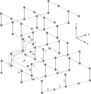
Figure 1: The 3D lattice: The four sites inside the loop (marked 1 to 4) constitute a unit cell; ${\bf a}_{1},{\bf a}_{2}$ and ${\bf a}_{3}$ are the basis vectors. Plaquette $p$ consists of sites marked 1 to 10.

The Hamiltonian is defined on the lattice shown in Fig. 1. For details about the lattice we refer to Ref. Mandal and Surendran, 2009. Here we just note that the coordination number is three and the links, which connect neighboring sites, are labeled $x$, $y$ or $z$. In addition, the three links at each site have different labels. The Hamiltonian is

$$H=-J_{x}\sum_{<i,j>_{x}}\sigma_{i}^{x}\sigma_{j}^{x}-J_{y}\sum_{<i,j>_{y}}\sigma_{i}^{y}\sigma_{j}^{y}-J_{z}\sum_{<i,j>_{z}}\sigma_{i}^{z}\sigma_{j}^{z},$$ (1)

where $\sigma^{a}_{i}$ are the Pauli matrices at site $i$ and $\sum_{<i,j>_{a}}$ denotes summation over $a$-type links.

The above Hamiltonian can be solved exactlyMandal and Surendran (2009) using a Majorana fermion representation of Pauli matricesKitaev (2006). The excitation spectrum is gapless when $J_{z}\leq J_{x}+J_{y}$, $J_{x}\leq J_{y}+J_{z}$, and $J_{y}\leq J_{z}+J_{x}$. Everywhere else in the parameter space there is a gap. The purpose of this paper is to study the nature of low-energy excitations in the gapped phase. Specifically, we will concentrate on the limit $J_{z}\gg J_{x},J_{y}$.

Let $H_{0}$ be the Hamiltonian obtained by putting $J_{x}=J_{y}=0$ in Eq. (1); it corresponds to isolated $z$-links and the spectrum is trivially solved. The ground state has a large degeneracy: any state in which the two spins in any given $z$-link, say, connecting sites $i$ and $j$, are either $|\uparrow\uparrow\rangle_{ij}$ or $|\downarrow\downarrow\rangle_{ij}$ has the minimum energy. Here $\sigma_{i}^{z}|\uparrow\rangle_{i}=|\uparrow\rangle_{i}$, $\sigma_{i}^{z}|\downarrow\rangle_{i}=-|\downarrow\rangle_{i}$, and similarly for $j$.

For small values of $J_{x}$ and $J_{y}$, the low energy excitations (more precisely, those eigenstates of $H$ adiabatically evolving from the degenerate ground states of $H_{0}$, as $J_{x}$ and $J_{y}$ are turned on) are described by an effective Hamiltonian $H_{eff}$ acting on this degenerate subspace (denoted by $\mathcal{H}_{0}$). Such an effective Hamiltonian will be defined on the lattice formed by the $z$-links, which we call $\mathcal{L}_{eff}$, and it turns out to be the diamond lattice, as far as the connectivity is concerned (see Fig. 2). $\mathcal{L}_{eff}$, which has coordination number four, is obtained from the original lattice by shrinking each $z$-link to its mid-point.

The links in $\mathcal{L}_{eff}$ lie along four different directions. We can choose an orthogonal coordinate system such that these directions are $(1,0,1),~{}(-1,0,1),~{}(0,-1,-1)$ and $(0,1,-1)$. We label the links respectively as $a,b,c$ and $d$. (Note that the links are not directed; positive and negative directions are equivalent.) Then at each site, the four links have four different labels.

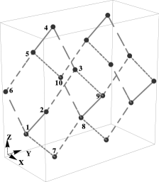
Figure 2: The lattice $\mathcal{L}_{eff}$ (diamond lattice) on which the effective Hamiltonian is defined. Bold, long-dashed, medium-dashed and short-dashed lines respectively denote links with labels $a,b,c$ and $d$.

Let $I$ denote the sites of $L_{eff}$. $\mathcal{H}_{0}$ is spanned by the states $\big{\{}\prod_{I}|m_{I}\rangle_{I}~{}|~{}m_{I}\in\{+,-\}\big{\}}$, where $|+\rangle_{I}\equiv|\uparrow\uparrow\rangle_{I}$ and $|-\rangle_{I}\equiv|\downarrow\downarrow\rangle_{I}$. The local degrees of freedom acting on $\mathcal{H}_{0}$ are effective spin-$\frac{1}{2}$ operators $\tau^{\alpha}_{I}$ ($\alpha\in\{x,y,z\}$) defined by

$$\tau_{I}^{z}|+\rangle_{I}=|+\rangle_{I}, \tau_{I}^{z}|-\rangle_{I}=-|-\rangle_{I},$$

$$\tau_{I}^{x}|+\rangle_{I}=|-\rangle_{I}, \tau_{I}^{x}|-\rangle_{I}=-|+\rangle_{I}.$$ (2)

Before writing down $H_{eff}$, it is convenient to define a loop operator as follows. Consider a loop $l$ in $\mathcal{L}_{eff}$ of length $n$ and consisting of sites $\{I_{k}|k=1,2,\dots n\}$ such that $I_{k}$ and $I_{k+1}$ are nearest neighbors, with the identification $I_{n+1}=I_{1}$. Let $\gamma_{k}$ denote the link connecting sites $I_{k}$ and $I_{k+1}$. We then define

$$B_{l}=\prod_{k=1}^{n}\tau_{I_{k}}^{\alpha_{k}},$$ (3)

where $\alpha_{k}$ is determined by the labels of the links $\gamma_{k-1}$ and $\gamma_{k}$ as follows:

$$\alpha_{k}=x \mbox{for labels $(a,c)$ and $(b,d)$},$$

$$\alpha_{k}=y \mbox{for $(a,d)$ and $(b,c)$},$$

$$\alpha_{k}=z \mbox{for $(a,b)$ and $(c,d)$}.$$ (4)

Here we need to consider only pairs with different labels since $\gamma_{k-1}$ and $\gamma_{k}$ are both links involving site $k$ and all links at a given site have different labels. It is easy to see that, with this definition, for any two loops $l$ and $l^{\prime}$,

$$[B_{l},B_{l^{\prime}}]=0.$$ (5)

This can be understood as follows. First, note from Eqs. (II) that $\alpha_{k}$ is the same for two pairs of labels if and only if they are complementary to each other. Now, $l$ and $l^{\prime}$ can intersect each other at one or more sites, and they can also have overlapping segments. Let $I$ be a site where they intersect. Then the two pairs of labels for the links that meet at $I$, corresponding to $l$ and $l^{\prime}$, will be complementary to each other and therefore $\alpha_{k}$ will be the same for both the loops. Now consider a segment where they overlap. Again, $\alpha_{k}$ will be the same for $l$ and $l^{\prime}$ everywhere on the segment except at the two end points, where they are strictly different. This is true for any overlapping segment of $l$ and $l^{\prime}$, which in turn means that among those sites shared by the two loops, there will be an even number of them where $\alpha_{k}$ is different for the two loops. This implies Eq. (5) since $\tau_{I}^{a}\tau_{I}^{b}=-\tau_{I}^{b}\tau_{I}^{a}$ when $a\neq b$.

To lowest order in $J_{x}$ and $J_{y}$, $H_{eff}$ is given in terms of the above operators corresponding to the smallest loops in $\mathcal{L}_{eff}$. We call such loops plaquettes and use the index $p$ to denote them. A plaquette consists of six sites and there are four types, each type corresponding to a particular label sequence and orientation. The four possible sequences are $acbacb$ (type-1), $cadcad$ (type-2), $bdabda$ (type-3) and $dbcdbc$ (type-4). In Fig. 2, $\{1,2,3,4,5,6\}$, $\{7,8,9,3,2,1\}$, $\{8,10,5,4,3,9\}$ and $\{7,1,6,5,10,8\}$ are respective examples.

In terms of the plaquette operators, the lowest order effective Hamiltonian is Mandal and Surendran (2009)

$$H_{eff}=-\frac{7}{256J_{z}^{5}}\left(J_{x}^{4}J_{y}^{2}\sum_{p}B_{p}+J_{x}^{2}J_{y}^{4}{\sum_{p}}^{\prime}B_{p}\right),$$ (6)

where the unprimed sum is over plaquettes of type- $1$ and $2$, while the primed sum is over plaquettes of type- $3$ and $4$.

III Excitations

Since all plaquette operators commute among themselves [see Eq. (5)], $H_{eff}$ is, in principle, trivially diagonalized. The energy eigenstates are then labeled by the eigenvalues of $B_{p}$, which are $+1$ or $-1$. However, not all $B_{p}$ are independent. In fact, it is the constraints existing among them that make $H_{eff}$ nontrivial and give rise to topological excitations.

Next we write down all the constraints and then find the allowed configurations of $B_{p}$ that are consistent with the constraints. In the process we will also calculate the ground state degeneracy. From now on we assume periodic boundary conditions in all three directions.

We first find a complete set of mutually commuting conserved operators that includes a maximal number of plaquette operators. To this end, we define a product of two loops. For our purposes, it is convenient to represent a loop by the set of links it contains. Let $l_{1}=\{\gamma_{1},\gamma_{2},\dots\gamma_{n_{1}}\}$ and $l_{2}=\{\delta_{1},\delta_{2},\dots\delta_{n_{2}}\}$ be two loops in $\mathcal{L}_{eff}$ containing $n_{1}$ links (denoted $\gamma_{i}$) and $n_{2}$ links (denoted $\delta_{i}$) respectively. The product of $l_{1}$ and $l_{2}$ is then defined as

$$l_{12}\equiv l_{1}\cdot l_{2}=l_{1}\cup l_{2}-l_{1}\cap l_{2}.$$ (7)

That is, $l_{12}$ is the loop formed by the links contained in $l_{1}$ or $l_{2}$ but without those links common to both. Then it is easy to check that

$$B_{l_{12}}=B_{l_{1}}\cdot B_{l_{2}}.$$ (8)

Therefore, to form a complete set of conserved operators we need to consider only the elementary plaquettes, but not any loop that can be obtained by combining a subset of the latter. There are three topologically nontrivial (noncontractible) loops corresponding to the three directions, which cannot be obtained from the plaquettes; we denote them $C_{x}$, $C_{y}$ and $C_{z}$ respectively. Any loop in the lattice can be obtained by combining the plaquettes and the three noncontractible loops. However, as we stated earlier, the plaquettes themselves are not all independent. There are three types of constraints that plaquette operators satisfy.

Local constraints.

It follows from Eq. (8) that the product of any set of plaquettes that forms a closed surface equals 1. The smallest such surface is formed by four adjacent plaquettes, any two of which share two links, as shown in Fig. 2. We call the volume enclosed by such a surface a basic cell. There are $N$ basic cells, where $N$ is the number of sites. This gives rise to $N-1$ independent constraints; it is $N-1$ because the constraint corresponding to any one basic cell equals the product of the constraints corresponding to the remaining $N-1$.

Surface constraints.

As a consequence of Eq. (8) there are three further constraints, independent of the local constraints, which correspond to the three topologically nontrivial surfaces.

Volume constraints.

Any product of corner sharing plaquettes that fill out the whole lattice equals one. There is only one such independent constraint.

Putting everything together, the total number of constraints is $N+3$. There are $2N$ plaquettes and the number of independent plaquette operators is $N-3$. These along with the three noncontractible loop operators $C_{x}$, $C_{y}$ and $C_{z}$ form a complete set of $N$ commuting operators.

There is another set of conserved operators corresponding to noncontractible surfaces. Such an operator can be defined on a plane $S$ that divides the lattice without cutting any links in such a way that at each site lying on the plane, two of the links lie on one side of the plane and the remaining two on the other. Then the surface operator is defined as follows:

$$M_{S}=\prod_{I\in S}\tau_{I}^{\alpha_{I}},$$ (9)

where the product is over sites lying on $S$ and $\alpha_{I}$ is determined by the two incoming (or outgoing) links according to the rule given in Eq. (II). $M_{S}$ commutes with all contractible loop operators because noncommuting—in our case, anticommuting—contributions come only at points where the loop pierces the surface and there will be an even number of such points. There are three such operators corresponding to the planes normal to $x$, $y$ and $z$ direction. We denote them $M_{X}$, $M_{y}$ and $M_{z}$, respectively.

Just as we obtained loop operators as a product of link-sharing plaquette operators, we can construct conserved ‘surface’ operators by multiplying corner sharing plaquette operators. In such a product, contribution from a shared site cancel out since it will be the same Pauli matrix for the two plaquettes sharing it [owing to Eq. (II)]. As a result the product will only involve sites that are not shared. Consequently, when corner sharing plaquettes fill out a certain volume in the lattice, the contribution to the operator will come only from the sites on the boundary.

The set of noncontractible loop and surface operators $C_{x}$, $C_{y}$, $C_{z}$ and $M_{X}$, $M_{y}$, $M_{z}$ form a system of three spin-$\frac{1}{2}$ degrees of freedom since

$$C_{a}M_{a}=-M_{a}C_{a}, C_{a}M_{b}=M_{b}C_{a}~{}\mbox{for}~{}a\neq b,$$

$$C_{a}C_{b}=C_{b}C_{a}, M_{a}M_{b}=M_{b}M_{a}.$$ (10)

It then follows that the ground state degeneracy is $2^{3}=8$, since the Hamiltonian does not depend on the above nonlocal operators. In fact, all excitations will have the same degeneracy of 8.

In the ground state $|GS\rangle$, $B_{p}=+1$ for all plaquettes. Evidently, all the constraints are satisfied. The excitations are obtained by flipping some of the $B_{p}$’s to $-1$. To find the configurations of $B_{p}$ that are consistent with the above constraints, it is useful to consider the lattice formed by the basic cells, each of which correspond to four plaquettes forming a closed surface. This lattice, denoted $\mathcal{L}_{p}$, is also the diamond lattice and the links in $\mathcal{L}_{p}$ represent the plaquettes in the original lattice.

In $\mathcal{L}_{p}$, the local constraints have a simple picture: the plaquette operators corresponding to the four links at each vertex multiply to 1. This implies that at every vertex only an even number of links (0, 2 or 4) can be flipped to -1, which in turn means that links with $B_{p}=-1$ form closed loops in $\mathcal{L}_{p}$. It is easy to see that any such loop excitation will also satisfy the surface constraints. However, the volume constraint imposes a further restriction on the allowed loop excitations.

The smallest loop in $\mathcal{L}_{p}$ is an elementary plaquette consisting of six links; we call it a 6-loop to distinguish it from the plaquette in $\mathcal{L}_{eff}$. Nevertheless, the excitation of an odd number of 6-loop violates the volume constraint. This can be shown by explicit construction, but there is another more transparent way to see this.

We have seen that the loop operators in Eq. (3) leave the ground state invariant. However, an open-string operator, obtained from a loop operator by truncation, i.e. by removing the part corresponding to a segment, is not conserved. The noncommuting part is at the ends of the string; it anticommutes with 6 of the $B_{p}$’s involving the spin at a given end. The plaquettes corresponding to these 6 $B_{p}$’s form a 6-loop in $\mathcal{L}_{p}$. An open-string operator then creates two 6-loop excitations at the ends. If two excited loops $l_{1}$ and $l_{2}$ overlap, then the resultant excitation will be along the loop $l_{12}$, which is the product of $l_{1}$ and $l_{2}$ [see Eq. (7)]. This is because the overlapping links are flipped twice—equivalent to no flip. Since any noncontractible loop $l$ can be expressed as a product of 6-loops, the excitation along $l$ can be created by exciting the corresponding 6-loops.

In the extreme case in which the string consists only of one site, say $I$, the corresponding string operator is $\tau_{I}^{x}$, $\tau_{I}^{y}$ or $\tau_{I}^{z}$. Then the two 6-loops at the ‘ends’ overlap (two of the links are shared), and the resultant excitation is an 8-loop. Since any state in the Hilbert space must be obtained from the ground state by the action of a combination of $\tau_{I}^{\alpha}$ operators, it follows that all states will have an even number of 6-loops, the elementary excitations.

However, a single 6-loop can be isolated by taking the other end of the string that creates it far away. This does not cost energy since the loops do not interact except when they overlap (then the overlapping part is annihilated). The energy of a loop is proportional to its length, which corresponds to the number of $B_{p}$’s excited.

In other words, the excitation spectrum has two superselection sectors: 1) the vacuum, which consists of states with an even number of 6-loop excitations and 2) the 6-loop, which consists of states with an odd number of 6-loop excitations.

In general, an excitation corresponds to a configuration of one or more loops in $\mathcal{L}_{p}$, where the loops can intersect but not overlap. As we have just shown, such an excitation is created by exciting the 6-loops into which the loop configuration can be decomposed. Let $L$ be a loop configuration and let $\Gamma$ be one of the decompositions of $L$ into 6-loops. It is straightforward to explicitly construct the operator that creates the excitation along $L$: arbitrarily pair up the constituent 6-loops; connect each pair by a string, again arbitrarily; then take the product of all the string operators that excite each pair.

Here it should be stressed that only the loop configuration $L$, on which the excitation lives, is physical. The state depends neither on the particular choice of decomposition $\Gamma$ nor on the specific way in which the 6-loops are paired and connected by strings. All choices give rise to the same state, up to a phase.

A loop excitation can also be interpreted as the edge of a membrane. Just as open-string operators are obtained by truncating a loop operator, we can construct an open-membrane operator by removing a patch from a closed-surface operator defined as a product of corner sharing plaquettes. Let $O_{M}$ be such an operator defined on a membrane $M$. As in the case of string operators, $O_{M}$ does not commute with the Hamiltonian. Nonetheless, it is only certain $B_{p}$’s along the edge of $M$ that do not commute with $O_{M}$; in fact, they anticommute. Therefore, in the state $O_{M}|GS\rangle$ these anticommuting $B_{p}$’s are excited; they will correspond to a loop in $\mathcal{L}_{P}$. In the language of the previous construction, $O_{M}$ corresponds to a specific choice of decomposition into 6-loops, which fixes $M$, and then neighboring 6-loops are paired together and connected by the shortest string between them, which consists of a single site.

IV Statistics

In this section, we determine the statistics obeyed by the excitations. We will see that the elementary 6-loop excitations are fermionic. Nontrivial phases also arise from braiding: when a 6-loop winds through a bigger loop, the state acquires a phase $\pi$.

IV.1 Localized excitations

A 6-loop excitation is the maximally localized state permitted by the constraints. So, they can be treated as particle-like and then one can ask whether they are fermions or bosons. We recall that in three dimensions there is no other statistics for point particles.

In a lattice, the statistics is determined by the algebra of the hopping operators Levin and Wen (2003). Let $i,j,k,l$ be four sites in the lattice and $\hat{t}_{\alpha\beta},~{}\alpha,\beta\in\{i,j,k,l\},$ be the corresponding hopping operators. Then,

$$\hat{t}_{lk}\hat{t}_{il}\hat{t}_{lj} = \hat{t}_{lj}\hat{t}_{il}\hat{t}_{lk}~{}\mbox{for bosons},$$

$$\hat{t}_{lk}\hat{t}_{il}\hat{t}_{lj} = -\hat{t}_{lj}\hat{t}_{il}\hat{t}_{lk}~{}\mbox{for fermions}.$$ (11)

A 6-loop in $\mathcal{L}_{p}$ represents 6 plaquettes in $\mathcal{L}_{eff}$, the lattice on which $H_{eff}$ is defined. In $\mathcal{L}_{eff}$, such a set of 6 plaquettes share a common link. Moreover, there is no other plaquette of which this particular link is part of. This provides a unique one-to-one mapping between links in $\mathcal{L}_{eff}$ and 6-loops in $\mathcal{L}_{p}$. Therefore 6-loop excitations can be thought of as localized around the links in $\mathcal{L}_{eff}$.

The above mapping gives a description of loops in $\mathcal{L}_{p}$ in terms of a link variable in $\mathcal{L}_{eff}$: it takes value $-1$ if the corresponding 6-loop is excited, otherwise, $+1$. This description, however, is redundant due to a $\mathbb{Z}_{2}$ gauge symmetry related to the non-uniqueness of the decomposition of a loop into 6-loops. The gauge transformation at a given site flips all the link variables connected to that site.

Figure 3: A site and the four links connected to it in the lattice $\mathcal{L}_{eff}$

Consider a site $I$ in $\mathcal{L}_{eff}$ and the four links emanating from it, denoted $i,j,k,l$ (see Fig. 3). In the previous section, we showed that $\tau_{I}^{\alpha}$ excites an 8-loop, which can be decomposed into two 6-loops. By the above mapping, this corresponds to a pair of links at $I$, the value of $\alpha$ determining which pair. Note that, due to the gauge symmetry, exciting a given pair or its complement are equivalent.

If $\tau_{I}^{\alpha}$ excites the links, say, $i$ and $j$, then it also hops an excitation between the two links. Without any loss of generality, we can assume that the links are labeled such that the hopping operators are

$$\hat{t}_{ij}=\hat{t}_{kl}=\tau_{I}^{x},$$

$$\hat{t}_{ik}=\hat{t}_{jl}=\tau_{I}^{y},$$

$$\hat{t}_{il}=\hat{t}_{jk}=\tau_{I}^{z}.$$ (12)

The first equality in each of the above equations follows from the gauge symmetry. Moreover, $\hat{t}_{ij}=\hat{t}_{ji}$. It immediately follows that

$$\hat{t}_{lk}\hat{t}_{il}\hat{t}_{lj}=-\hat{t}_{lj}\hat{t}_{il}\hat{t}_{lk}.$$ (13)

Therefore, 6-loops are fermions.

IV.2 Braiding

A configuration of loops can evolve along topologically distinct paths. The question one can ask then is whether there is a phase difference between distinct paths. We will now show that a phase $\pi$ is acquired when a 6-loop winds through a bigger loop.

Let $O_{M}$ be a membrane operator that creates an excitation along loop $l$.

$$O_{M}=\prod_{I\in M}\tau_{I}^{\alpha_{I}}.$$ (14)

Here $M$ is a set of sites $I$ which fills the surface enclosing $l$, and $\alpha_{I}$ is determined by the labels of the two incoming (or outgoing) links, according to Eq. (II).

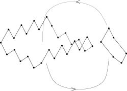
Figure 4: Schematic depiction of a fermionic 6-loop braiding through a bigger loop. Traversing such a path results in a topological phase $\pi$

A 6-loop is moved along a closed path by the loop operator corresponding to the path. A path which takes it through $l$ will have one site common with $M$. Here we take $l$ to be big enough so that the 6-loop can pass through without interacting, i.e., without touching (see Fig. 4). Let this site be $I_{c}$. The loop operator $B_{l}$ is given by

$$B_{l}=\prod_{I\in l}\tau_{I}^{\beta_{I}},$$ (15)

where $\beta_{I}$ are also determined by the set of rules in Eq. (II).

Since $l$ goes through the membrane, $\beta_{I_{c}}$ is determined by one outgoing and one incoming link; therefore, it is strictly different from $\alpha_{I_{C}}$. Hence

$$O_{M}B_{l}=-B_{l}O_{M}.$$ (16)

This results in a phase difference of $\pi$ between paths which go through $l$ and paths which do not.

V Summary and discussion

We have studied the gapped phase of 3D Kitaev model by analyzing the effective Hamiltonian $H_{eff}$ obtained in the limit of strong $z-$links. $H_{eff}$ is defined on the diamond lattice and the individual terms it contains are mutually commuting plaquette operators. There are loop and surface operators that are conserved. In the language of Levin and Wen Levin and Wen (2005), our model has both string-net and membrane-net condensation.

There is an embedded lattice $\mathcal{L}_{p}$, also a diamond lattice, in which the links stand for plaquettes. In $\mathcal{L}_{p}$, the excitations have the structure of loops. The energy of a loop is proportional to its length, consequently, the ground state is free of loops. The loops interact only when they overlap, in which case the overlapping part is annihilated. The smallest loops in $\mathcal{L}_{p}$, the 6-loops, are the elementary excitations and they obey fermionic statistics. The fermionic 6-loop braids nontrivially with a bigger loop: when it winds through the latter over a closed path, the wave function acquires a phase $\pi$.

Even though there already exists other exactly solvable models in 3D that are topologically ordered Levin and Wen (2003); Hamma et al. (2005); Bombin and Martin-Delgado (2007); Kim (2010), our model has a particular relevance in that it is obtained as the effective Hamiltonian for the gapped phase of 3D Kitaev model, which involves only two-spin interactions as opposed to higher-spin operators in the other solvable models. It will therefore be worthwhile to analyze the model at finite temperature to see if topological order survives Castelnovo and Chamon (2008); Hamma et al. (2009); Kim (2010).

References

- Kitaev (2006) A. Y. Kitaev, Ann. Phys. 321, 2 (2006).
- Kitaev (2003) A. Y. Kitaev, Ann. Phys. 303, 2 (2003).
- Duan et al. (2003) L. M. Duan, E. Demler, and M. D. Lukin, Phys. Rev. Lett. 91, 090402 (2003).
- Baskaran et al. (2007) G. Baskaran, S. Mandal, and R. Shankar, Phys. Rev. Lett. 98, 247201 (2007).
- Chen and Nussinov (2008) H.-D. Chen and Z. Nussinov, J. Phys. A: Math. Theor. 41, 075001 (2008).
- Schmidt et al. (2008) K. P. Schmidt, S. Dusuel, and J. Vidal, Phys. Rev. Lett. 100, 057208 (2008).
- Dusuel et al. (2008) S. Dusuel, K. P. Schmidt, and J. Vidal, Phys. Rev. Lett. 100, 177204 (2008).
- Baskaran et al. (2008) G. Baskaran, D. Sen, and R. Shankar, Phys. Rev. B 78, 115116 (2008).
- Sengupta et al. (2008) K. Sengupta, D. Sen, and S. Mondal, Phys. Rev. Lett. 100, 077204 (2008).
- Mandal and Surendran (2009) S. Mandal and N. Surendran, Phys. Rev. B 79, 024426 (2009).
- Si and Yu (2008) T. Si and Y. Yu, Nucl. Phys. B 803, 428 (2008).
- Ryu (2009) S. Ryu, Phys. Rev. B 79, 075124 (2009).
- Levin and Wen (2003) M. Levin and X.-G. Wen, Phys. Rev. B 67, 245316 (2003).
- Levin and Wen (2005) M. A. Levin and X.-G. Wen, Phys. Rev. B 71, 045110 (2005).
- Hamma et al. (2005) A. Hamma, P. Zanardi, and X.-G. Wen, Phys. Rev. B 72, 035307 (2005).
- Bombin and Martin-Delgado (2007) H. Bombin and M. A. Martin-Delgado, Phys. Rev. B 75, 075103 (2007).
- Kim (2010) I. H. Kim, arxiv:1012.0859 (2010).
- Castelnovo and Chamon (2008) C. Castelnovo and C. Chamon, Phys. Rev. B 78, 155120 (2008).
- Hamma et al. (2009) A. Hamma, C. Castelnovo, and C. Chamon, Phys. Rev. B 79, 245122 (2009).