Density-matrix approach for an interacting polariton system

Abstract

Using Lindblad approach we develop a general formalism for theoretical description of a spatially inhomogenous bosonic system with dissipation provided by the interaction of bosons with a phonon bath. We apply our results to model the dynamics of an interacting one dimensional polariton system in real space and time, analyzing in detail the role of polariton-polariton and polariton- phonon interactions.

I I. Introduction

A semiconductor microcavity is a photonic structure designed to enhance the light-matter interaction. In a planar microcavity photons are confined between two mirrors and resonantly interact with the excitonic transition of a two-dimensional semiconductor quantum well (QW). If the quality factor of the cavity is sufficiently high, it is possible to achieve the regime of strong coupling between the cavity photon and QW exciton. In this case the elementary excitations in the system, which are called cavity polaritons, have a hybrid, half-light, half-matter nature. The peculiar properties of polaritons make them a unique laboratory for studying of various collective phenomena interesting from the point of view of basic physics, which range from polariton BEC KasprzakNature , superfluidity AmoNature and Josephson effect LagoudakisJosephson to polariton-mediated superconductivity LaussySupercond .

Besides fundamental interest, quantum microcavities in the strong coupling regime can be used for a variety of optoelectronic applications Imamoglu . Recently, it was proposed that the peculiar spin structure and possibility to achieve lateral confinement of polaritons Confinement opens a way for creation of optical analogs of spintronic components (so-called spinoptronic devices), based on transport of cavity polaritons in real space. In this context, the analysis of one-dimensional (1D) polariton transport is of particular importance WertzNature , as 1D polariton channels are fundamental building blocks of such future spinoptronic devices as polariton neurons LiewNeuron and polariton integrated circuits LiewCircuit .

On the theoretical side, transport properties of exciton-polaritons in real space have not yet been studied in detail. Early works SpinHall ; Glazov ; ShelykhBerry treated the case of polaritons interacting with external potentials only neglecting both polariton-polariton and polariton-phonon interactions. However, in the most interesting regime of polariton BEC neither of the two interactions can in principle be neglected. Indeed, coupling of the polaritons with a reservoir of acoustic phonons leads to thermalization of the polariton subsystem, which is dramatically speeded up by polariton- polariton interactions which are known to be responsible for overcoming the so-called ”bottleneck effect” Bottleneck . Besides, in the regime of polariton BEC polariton-polariton interactions are responsible for the onset of superfluidity AmoNature .

Currently, there are two ways of describing a system of interacting polaritons. Assuming full coherence of the polariton system, polariton-polariton interactions can be accounted for using nonlinear Gross- Pitaevskii (GP) equation, satisfactorily describing the dynamics of inhomogeneous polariton droplets in real space and time Carusotto ; ShelykhGP . The approach, however, does not include interactions with a phonon bath, responsible for thermalization of the system and leading to dephasing. In the opposite limit, when the polariton system is supposed to be fully incoherent, its dynamics can be described using a system of semiclassical Boltzmann equations Porras2002 ; Kasprzak2008 ; Haug2005 ; Cao , which provides information about time dependence of the occupation numbers in reciprocal space but fails to describe real space dynamics in the inhomogeneous system.

Recently, there appeared theoretical attempts to combine the two mentioned approaches introducing dissipation terms into GP equation in a phenomenological way Wouters2007 . To our mind, however, these attempts, although being interesting and leading to a rich phenomenology BerloffVortex ; Tim1D , are not fully satisfactory, as they lack any microscopic justification. In the present paper we give an alternative way of describing the dynamics of an inhomogeneous polariton system in real space and time accounting for dissipation effects. Our consideration is based on Lindblad approach for density matrix dynamics. We use our results for modeling of the propagation of polariton droplets in 1D channels. It should be noted, that the method we develop is rather general and can in principle be applied to any system of interacting bosons in contact with a phonon reservoir (for example, indirect excitons Butov ). We have previously applied this formalism to model Josephson oscillations between two spatially separated condensates, but in that context the spatial dependence was trivial Josephson2010 .

II II. Formalism

We describe the state of the system (polaritons plus phonons) by its density matrix $\rho$, for which we apply Born approximation factorizing it into the phonon part which is supposed to be time-independent and corresponds to the thermal distribution of acoustic phonons $\rho_{ph}=\texttt{exp}\left\{-\beta\widehat{H}_{ph}\right\}$ and the polariton part $\rho_{pol}$ whose time dependence should be determined, $\rho=\rho_{ph}\otimes\rho_{pol}$. Our aim is to find dynamic equations for the time evolution of the single-particle polariton density matrix in real space.

$$\rho(\textbf{r},\textbf{r}^{\prime},t)=Tr\left\{\widehat{\psi}^{\dagger}(\textbf{r},t)\widehat{\psi}(\textbf{r}^{\prime},t)\rho\right\}\equiv\langle\widehat{\psi}^{\dagger}(\textbf{r},t)\widehat{\psi}(\textbf{r}^{\prime},t)\rangle$$ (1)

where $\widehat{\psi}^{\dagger}(\textbf{r},t),\widehat{\psi}(\textbf{r},t)$ are operators of the polariton field, and the trace is performed by all degrees of freedom of the system. The particularly interesting quantities are the diagonal matrix elements which give the density of the polariton field in real space and time $n(\textbf{r},t)=\rho(\textbf{r},\textbf{r},t)$. In our consideration we neglect the spin of the cavity polaritons for simplicity, as our main goal here is to account for dissipative dynamics coming from interaction with phonons, and spin degree of freedom is not expected to introduce any qualitatively new physics from this point of view. However, that introduction of spin into the model is straightforward and corresponding work is currently underway. It should also be noted that our model is to some extent similar to one proposed in Ref. WoutersWigner, . Differently from that paper, however, we assume that all decoherence in the system comes from the interaction with acoustic phonons which is neglected in Ref. WoutersWigner, and thus do not perform the separation of the polariton ensemble into coherent low energy part and incoherent high- energy reservoir.

It is convenient to go to reciprocal space, making a Fourier transform of the one-particle density matrix,

$$\rho(\textbf{k},\textbf{k}^{\prime},t) =(2\pi)^{d}/L^{d}\int e^{i(\textbf{kr}-\textbf{k}^{\prime}\textbf{r}^{\prime})}\rho(\textbf{r},\textbf{r}^{\prime},t)d\textbf{r}d\textbf{r}^{\prime}=$$ (2)

$$=Tr\left\{a_{\textbf{k}}^{+}a_{\textbf{k+q}}\right\}\equiv\langle a_{\textbf{k}}^{+}a_{\textbf{k}^{\prime}}\rangle$$

where $d$ is the dimensionality of the system ($d=2$ for non-confined polaritons, $d=1$ for the polariton channel), L is its linear size, $a_{\textbf{k}}^{+}$, $a_{\textbf{k}}$ are creation and annihilation operators of the polaritons with momentum k. Note, that we have chosen the prefactor in a Fourier transform in such a way, that the values of $\rho(\textbf{k},\textbf{k}^{\prime},t)$ are dimensionless, and diagonal matrix elements give occupation numbers of the states in discretized reciprocal space. Knowing the density matrix in reciprocal space, we can find the density matrix in real space straightforwardly applying inverse Fourier transform.

The total Hamiltonian of the system can be represented as a sum of two parts,

$$H=H_{1}+H_{2}$$ (3)

where the first term $H_{1}$ describes the ”coherent” part of the evolution, corresponding to free polariton propagation and polariton-polariton interactions and the second term $H_{phon}$ corresponds to the dissipative interaction with acoustic phonons. The two terms affect the polariton density matrix in a qualitatively different way.

II.1 A. Polariton-polariton interactions

The part of the evolution corresponding to $H_{1}$ is given by the following expression

$$H_{1}=\sum_{\textbf{k}}E_{\textbf{k}}a_{\textbf{k}}^{+}a_{\textbf{k}}+\frac{U}{2}\sum_{\textbf{k}_{1},\textbf{k}_{2},\textbf{p}}a_{\textbf{k}_{1}}^{+}a_{\textbf{k}_{2}}^{+}a_{\textbf{k}_{1}+\textbf{p}}a_{\textbf{k}_{2}-\textbf{p}}$$ (4)

where $E_{\textbf{k}}$ is the energy dispersion of the polaritons, $U$ is the matrix element of the polariton-polariton interactions. In the current paper we neglect the p-dependence of the polariton- polariton interaction constant coming from Hopfield coefficients polpol . We do this approximation because the goal of the manuscript is to present a novel formalism for description of the relaxation effects and not detailed modeling of a particular experiment, and we want to keep our formalism as simple as possible. Besides, this approximation is widely used in current description of polaritonic systems based on modifications of the Gross-Pitaevskii equations Wouters2007 ; BerloffVortex ; Tim1D . However, for modeling of realistic experiments the p-dependence of the interaction constant can easily be introduced into the equations.

The effect of $H_{1}$ on the evolution of the density matrix is described by the Liouville-von Neumann equation,

$$i\left(\partial_{t}\rho\right)^{(1)}=\left[H_{1};\rho\right]$$ (5)

which after use of mean field approximation leads to the following dynamic equations for the elements of the single-particle density matrix in reciprocal space (see Appendix I for details of the derivation):

$$\left\{\partial_{t}\rho(\textbf{k},\textbf{k})\right\}^{(1)}=2U\sum_{\textbf{k}_{1},\textbf{p}}\textrm{Im}\left\{\rho(\textbf{k}_{1},\textbf{k}_{1}-\textbf{p})\rho(\textbf{k},\textbf{k}+\textbf{p})\right\}$$ (6)

$$\left\{\partial_{t}\rho(\textbf{k},\textbf{k}^{\prime})\right\}^{(1)}=i(E_{\textbf{k}}-E_{\textbf{k}}^{\prime})\rho(\textbf{k},\textbf{k}^{\prime})+$$ (7)

$$+iU\sum_{\textbf{k}_{1},\textbf{p}}\rho(\textbf{k}_{1},\textbf{k}_{1}-\textbf{p})\left[\rho(\textbf{k}-\textbf{p},\textbf{k}^{\prime})-\rho(\textbf{k},\textbf{k}^{\prime}+\textbf{p})\right]$$

These expressions represent an analog of the Gross-Pitaevskii equation written for the density matrix.

II.2 B. Scattering with acoustic phonons

Polariton-phonon scattering corresponds to the interaction of the quantum polariton system with a classical phonon reservoir. It is of dissipative nature, and thus straightforward application of the Liouville-von Neumann equation is impossible. Introduction of dissipation into quantum systems is an old problem, for which there is no single well established solution. In the domain of quantum optics, however, there are standard methods based on the Master Equation techniques Carmichael . In the following we give a brief outline of this approach applied to a dissipative polariton system.

The Hamiltonian of interaction of polaritons with acoustic phonons in Dirac representation can be represented as

$$\widehat{H}_{2}(t)=H^{-}(t)+H^{+}(t)=$$ (8)

$$=\sum_{\textbf{k},\textbf{q}}D(\textbf{q})e^{i(E_{\textbf{k}+\textbf{q}}-E_{\textbf{k}})t}a_{\textbf{k}+\textbf{q}}^{+}a_{\textbf{k}}(b_{\textbf{q}}e^{-i\omega_{\textbf{q}}t}+b_{-\textbf{q}}^{+}e^{i\omega_{\textbf{q}}t})$$

where $a_{\textbf{k}}$ are operators for polaritons, $b_{\textbf{q}}$ operators for phonons, $E_{\textbf{k}}$ and $\omega_{\textbf{q}}$ are dispersion relations for polaritons and acoustic phonons respectively, $D(\textbf{q})$ is the polariton-phonon coupling constant. In the last equality we separated the terms $H^{+}$ where a phonon is created, containing the operators $b^{+}$, from the terms $H^{-}$ in which it is destroyed, containing operators $b$.

Now, one can consider a hypothetical situation when polariton-polariton interactions are absent, and all redistribution of the polaritons in reciprocal space is due to the scattering with a thermal reservoir of acoustic phonons. One can rewrite the Liouville-von Neumann equation in an integro-differential form and apply the so called Markovian approximation, corresponding to the situation of fast phase memory loss (see Ref. Carmichael, for the details and discussion of limits of validity of the approximation)

$$\left(\partial_{t}\rho\right)^{(2)} =-\int_{-\infty}^{t}dt^{\prime}\left[H_{2}(t);\left[H_{2}(t^{\prime});\rho(t)\right]\right]=$$ (9)

$$=\delta_{\Delta E}\left[2\left(H^{+}\rho H^{-}+H^{-}\rho\right.H^{+}\right)-$$

$$\left.-\left(H^{+}H^{-}+H^{-}H^{+}\right)\rho-\rho\left(H^{+}H^{-}+H^{-}H^{+}\right)\right]$$

where the coefficient $\delta_{\Delta E}$ denotes energy conservation and has dimensionality of inverse energy and in the calculation taken to be equal to the broadening of the polariton state KavokinMalpuech . For time evolution of the mean value of any arbitrary operator $\langle\widehat{A}\rangle=Tr(\rho\widehat{A})$ due to scattering with phonons one thus has (derivation of this formula is represented in Appendix II):

$$\left\{\partial_{t}\langle\widehat{A}\rangle\right\}^{(2)}=\delta_{\Delta E}\left(\langle[H^{-};[\widehat{A};H^{+}]]\rangle+\langle[H^{+};[\widehat{A};H^{-}]]\rangle\right).$$ (10)

Putting $\widehat{A}=a_{\textbf{k}}^{+}a_{\textbf{k}^{\prime}}$ in this equation we get the contributions to the dynamic equations for the elements of the single-particle density matrix coming from polariton-phonon interaction (see Appendix III):

$$\left\{\partial_{t}\rho(\textbf{k},\textbf{k})\right\}^{(2)} =$$ (11)

$$\sum_{\textbf{q}^{\prime},E_{\textbf{k}}<E_{\textbf{k+q}^{\prime}}} 2W(\textbf{q}^{\prime})\left[\rho(\textbf{k+q}^{\prime},\textbf{k+q}^{\prime})(n_{\textbf{q}^{\prime}}^{ph}+1)(\rho(\textbf{k},\textbf{k})+1)\right.$$

$$\left.-\rho(\textbf{k},\textbf{k})n_{\textbf{q}^{\prime}}^{ph}(\rho(\textbf{k+q}^{\prime},\textbf{k+q}^{\prime})+1)\right]+$$

$$+\sum_{\textbf{q}^{\prime},E_{\textbf{k}}>E_{\textbf{k+q}^{\prime}}} 2W(\textbf{q}^{\prime})\left[\rho(\textbf{k+q}^{\prime},\textbf{k+q}^{\prime})n_{-\textbf{q}^{\prime}}^{ph}(\rho(\textbf{k},\textbf{k})+1)-\right.$$

$$\left.-\rho(\textbf{k},\textbf{k})(n_{-\textbf{q}^{\prime}}^{ph}+1)(\rho(\textbf{k+q}^{\prime},\textbf{k+q}^{\prime})+1)\right]$$

and

$$\left\{\partial_{t}\rho(\textbf{k},\textbf{k}^{\prime})\right\}^{(2)}=\rho(\textbf{k},\textbf{k}^{\prime})\times$$ (12)

$$\times\left\{\sum_{\textbf{q}^{\prime},E_{\textbf{k}}<E_{\textbf{k+q}^{\prime}}}W(\textbf{q}^{\prime})\left[\rho(\textbf{k+q}^{\prime},\textbf{k+q}^{\prime})-n_{\textbf{q}^{\prime}}^{ph}\right]+\right.$$

$$+ \sum_{\textbf{q}^{\prime},E_{\textbf{k}}>E_{\textbf{k+q}^{\prime}}}W(\textbf{q}^{\prime})\left[-\rho(\textbf{k+q}^{\prime},\textbf{k+q}^{\prime})-n_{\textbf{q}^{\prime}}^{ph}-1\right]+$$

$$+ \sum_{\textbf{q}^{\prime},E_{\textbf{k}}^{\prime}<E_{\textbf{k}^{\prime}+\textbf{q}^{\prime}}}W(\textbf{q}^{\prime})\left[\rho(\textbf{k}^{\prime}+\textbf{q}^{\prime},\textbf{k}^{\prime}+\textbf{q}^{\prime})-n_{\textbf{q}^{\prime}}^{ph}\right]+$$

$$+ \left.\sum_{\textbf{q}^{\prime},E_{\textbf{k}}^{\prime}>E_{\textbf{k}^{\prime}+\textbf{q}^{\prime}}}W(\textbf{q}^{\prime})\left[-\rho(\textbf{k}^{\prime}+\textbf{q}^{\prime},\textbf{k}^{\prime}+\textbf{q}^{\prime})-n_{\textbf{q}^{\prime}}^{ph}-1\right]\right\}$$

where the transition rates are given by $W(\textbf{q})=D^{2}(\textbf{q})\delta_{\Delta E_{\textbf{q}}}$ and $n_{\textbf{q}}^{ph}$ denote the occupation numbers of phonons with wavevector q given by Bose distribution.

Eq. (11) is nothing but a standard Boltzmann equation for the phonon-assisted polariton relaxation, while Eq. (12) describes the decay of the off-diagonal matrix elements of a single-particle density matrix due to interaction with classical phonon reservoir. Together these equations thus describe thermalization of the polariton system.

To account for the effects of free polariton propagation, polariton-polariton and polariton-phonon interactions one should combine together expressions (6), (7), (11) and (12). After finding the single-particle density matrix in reciprocal space by solving the corresponding dynamic equations, one can determine the dynamic of the system in real space simply performing a Fourier transformation by k and k’ variables.

III III. Results and discussion

Our formalism is suitable for the description of both 2D polaritons and polaritons confined within 1D channels. In this paper we present the results of numerical modeling for the latter case only, as solving of the dynamic equations for 2D case requires the use of supercomputing facilities.

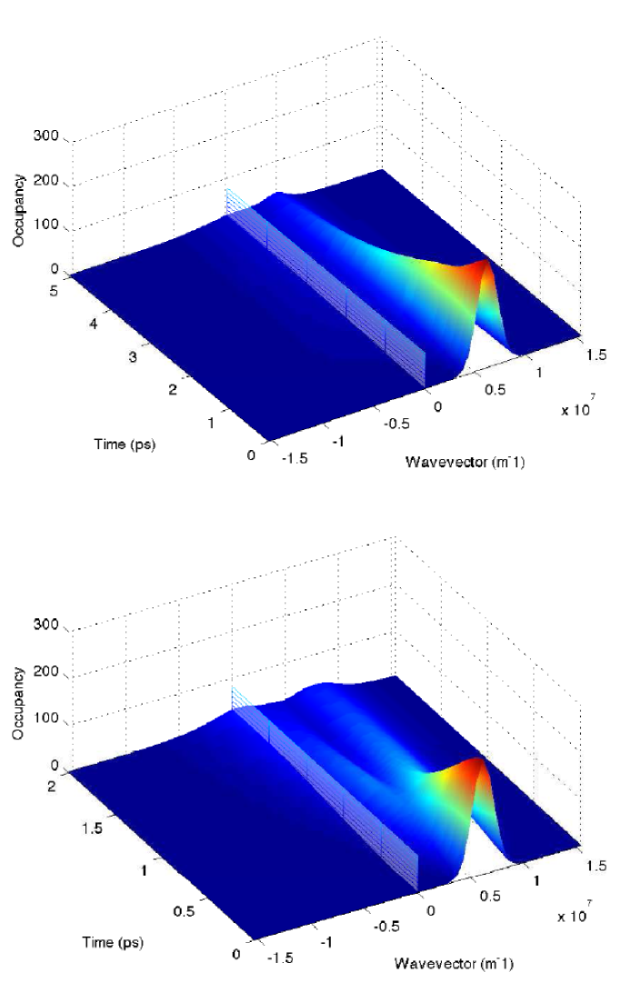
Figure 1: Time evolution of polariton distribution in $k$-space. The vertical plane denotes $k=0$ state. a) Only polariton-phonon scattering is accounted for. The relaxation towards $k=0$ state is blocked due to the bottleneck effect. b) Both polariton-phonon and polariton-polariton scattering are accounted for. The maximum of the polariton concentration is developed at $k=0$, signifying the overcoming of the bottleneck effect. Another maximum appears at higher $k$, due to the energy-conserving nature of the polariton-polariton interactions.

The results of modeling are shown on Figures 1-3. We consider a $2$ $\mu$m wide polariton channel in GaAs microcavity with Rabi splitting 15 meV at temperature $T=1$ K. The polaritons are created by a short coherent localized laser pulse. We account for the finite lifetime of cavity polaritons $\tau=5$ ps adding the term $-\rho(\textbf{k},\textbf{k}^{\prime})/\tau$ into the dynamic equations.

Figure 1 shows the dynamics of the polariton system in reciprocal space and demonstrates the roles of the polariton-phonon and polariton-polariton interactions. If only the former are included, the system demonstrates the bottleneck effect shown on Fig. 1a. Due to the energy relaxation coming from the interactions with phonons, polaritons have a tendency to move towards the ground state in $k$-space. However, this process is dramatically slowed down in the inflection region of the polariton dispersion, where polariton-phonon interaction becomes inefficient. Consequently, there is no remarkable increase of the population of $k=0$ state Bottleneck . The bottleneck effect can be overcome by the polariton-polariton interactions, as shown on Fig. 1b. One sees that in this case the particles accumulate quickly in $k=0$ state. At the same time, the second maximum of the polariton distibution appears at higher $k$ due to the energy conservative nature of the polariton-polariton interactions (analogically to the formation of the idler mode in polariton parametric oscillator PPO ).

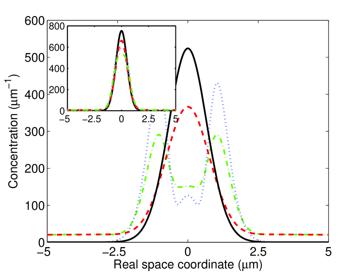
Figure 2: Polariton distribution in real space at times $t=0.5$ ps (inset) and $t=1.5$ ps after creating the package by a localized laser pulse centered around $k=0$. Black solid line corresponds to ballistic propagation, red dashed line - to polariton-phonon interactions, blue dotted line - to polariton-polariton interactions and green dashed line - to both polariton-phonon and polariton-polariton interactions.

Our results for the dynamics of the polariton distribution in reciprocal space are in good agreement with those obtained by using Boltzmann equations. In addition, our approach allows consideration of the dynamics of the dissipative polariton system in real space. This is illustrated on Figures 2 and 3.

Figure 2 shows the effect of the various types of interactions on the real space dynamics of the localized polariton wavepackage. We compare the cases of the ballistic propagation with those where only polariton-phonon interactions are included, only polariton-polariton interactions are included and both polariton-polariton and polariton-phonon interactions are included. As one sees, the dynamics are very different for these four cases. Polariton-polariton interactions lead to splitting of the wavepackage into two soliton- like peaks, which is in good qualitative agreement with the results given by Gross-Pitaevskii equation ShelykhGP . On the other hand, polariton-phonon interactions lead to damping of the package, contributing to the recovering of the homogenious distribution of the polaritons in real space as it is expected from the classical diffusion equation.

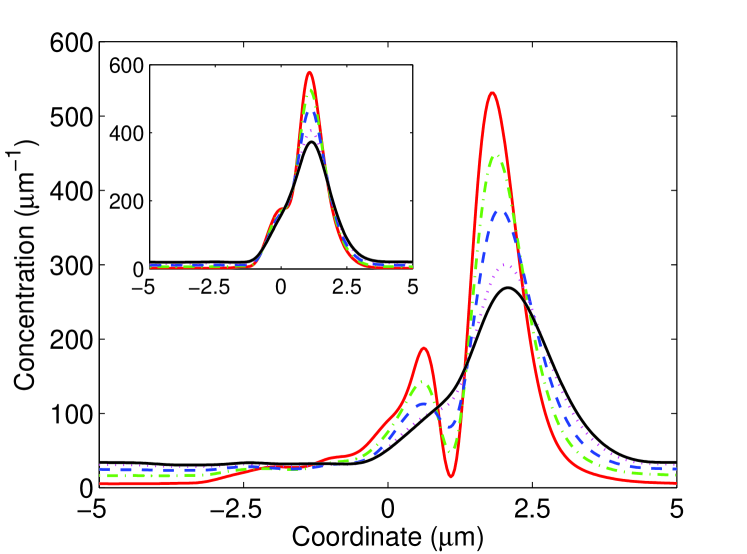
Figure 3: Polariton distribution in real space at times $t=0.5$ ps (inset) and $t=1.5$ ps after creating the package by a localized laser pulse centered around $k=3\cdot 10^{6}$ m^-1. Scattering on phonons and polaritons are both accounted for. The temperatures are: 1 K (red/solid), 4 K (green/dash-dot), 8 K (blue/dashed), 15 K (magenta/dotted) and 20 K (black/solid).

Naturally, the effect of the phonon damping strongly depends on temperature, as shown on Fig. 3. One sees, that at low temperatures the propagating package is split into two due to the polariton-polariton interactions. Increasing the temperature smoothes down the polariton distibution and at $T=20K$ one has just a single peak.

IV IV. Conclusion

In conclusion, we developed a formalism for the description of the dissipative dynamics of an inhomogeneous polariton system in real space and time accounting for polariton-polariton interactions and polariton-phonon scattering. The formalism was applied for numerical modeling of the propagation of a polariton droplet in a 1D channel. Our approach can also be used for modeling the dissipative dynamics of other bosonic systems (e.g. indirect excitons).

V Acknowledgements

We thank G. Malpuech, D.D. Solnyshkov and T.C.H. Liew for useful discussions. The work was supported by Rannis ”Center of excellence in polaritonics” and FP7 IRSES projects ”SPINMET” and ”POLAPHEN”.

VI Appendix I: derivation of kinetic equations for polariton- polariton scattering

The evaluation of the dynamic equations of $\langle a_{\textbf{k}}^{\dagger}a_{\textbf{k}}\rangle$ and $\langle a_{\textbf{k}}^{\dagger}a_{\textbf{k+q}}\rangle$ using Eq. (5) and applying the mean field approximation gives:

$$\textrm{Tr}\left\{a_{\textbf{k}}^{+}a_{\textbf{k+q}}\left[\rho;H_{p-p}\right]\right\} =U\sum_{\textbf{k}_{1},\textbf{k}_{2},\textbf{p}}\rho(\textbf{k}_{2},\textbf{k}_{2}-\textbf{p})\textrm{Tr}\left\{a_{\textbf{k}}^{+}a_{\textbf{k+q}}\left[\rho;a_{\textbf{k}_{1}}^{+}a_{\textbf{k}_{1}+\textbf{p}}\right]\right\}=$$ (13)

$$=U\sum_{\textbf{k}_{2},\textbf{p}}\rho(\textbf{k}_{2},\textbf{k}_{2}-\textbf{p})\left[-\rho(\textbf{k},\textbf{k+q+p})+\rho(\textbf{k-p},\textbf{k+q})\right]$$

$$\textrm{Tr}\left\{a_{\textbf{k}}^{+}a_{\textbf{k}}\left[\rho;H_{p-p}\right]\right\}=U\sum_{\textbf{k}_{1},\textbf{k}_{2},\textbf{p}}\rho(\textbf{k}_{2},\textbf{k}_{2}-\textbf{p})\textrm{Tr}\left\{a_{\textbf{k}}^{+}a_{\textbf{k}}\left[\rho;a_{\textbf{k}_{1}}^{+}a_{\textbf{k}_{1}+\textbf{p}}\right]\right\}=$$ (14)

$$=U\sum_{\textbf{k}_{1},\textbf{k}_{2},\textbf{p}}\rho(\textbf{k}_{2},\textbf{k}_{2}-\textbf{p})\textrm{Tr}\left\{\rho\left[a_{\textbf{k}_{1}}^{+}a_{\textbf{k}_{1}+\textbf{p}}a_{\textbf{k}}^{+}a_{\textbf{k}}-a_{\textbf{k}}^{+}a_{\textbf{k}}a_{\textbf{k}_{1}}^{+}a_{\textbf{k}_{1}+\textbf{p}}\right]\right\}=-2iU\sum_{\textbf{k}_{2},\textbf{p}}\textrm{Im}\left\{\rho(\textbf{k}_{2},\textbf{k}_{2}-\textbf{p})\rho(\textbf{k},\textbf{k+p})\right\}$$

From this one straightforwardly gets Eqs. 6, 7.

VII Appendix II: Derivation of expression for dynamics of mean values in Born- Markov approximation

Now, consider the evolution of a mean value of any arbitrarty operator $A,\langle A\rangle=Tr(\rho A)$ (energy conserving delta-function omitted) if dynamics of a density matrix is given by Eq. 9:

$$\partial_{t}\langle A\rangle =\texttt{Tr}\left(2H^{+}\rho H^{-}A+2H^{-}\rho H^{+}A-\left(H^{+}H^{-}+H^{-}H^{+}\right)\rho A-\rho\left(H^{+}H^{-}+H^{-}H^{+}\right)A\right)=$$ (15)

$$=\texttt{Tr}\left[\rho\left(2H^{-}AH^{+}+2H^{+}AH^{-}-A\left(H^{+}H^{-}+H^{-}H^{+}\right)-\left(H^{+}H^{-}+H^{-}H^{+}\right)A\right)\right]$$

where we used the property of the invariance of the trace as regards cyclic permutations of operators. The latter expression can be simplified as

$$2H^{-}AH^{+}+2H^{+}AH^{-}-A\left(H^{+}H^{-}+H^{-}H^{+}\right)-\left(H^{+}H^{-}+H^{-}H^{+}\right)A=$$ (16)

$$={} 2H^{-}([A;H^{+}]+H^{+}A)+2H^{+}([A;H^{-}]+H^{-}A)-A\left(H^{+}H^{-}+H^{-}H^{+}\right)-\left(H^{+}H^{-}+H^{-}H^{+}\right)A=$$

$$={} 2H^{-}[A;H^{+}]+2H^{+}[A;H^{-}]-H^{+}[A;H^{-}]-[A;H^{+}]H^{-}-H^{-}[A;H^{+}]-[A;+H^{-}]H^{+}=$$

$$={} [H^{-};[A;H^{+}]]+[H^{+};[A;H^{-}]]$$

where we used the following property of commutators: $[A;BC]=B[A;C]+[A;B]C$. Thus

$$\partial_{t}\langle A\rangle=\texttt{Tr}\left(\rho[H^{-};[A;H^{+}]]\right)+\texttt{Tr}\left(\rho[H^{+};[A;H^{-}]]\right)$$ (17)

For the important case of the Hermitian operator A corresponding to a physical observable one has

$$[H^{-};[A;H^{+}]]^{+}=-[[A;H^{+}]^{+};H^{+}]=$$ (18)

$$={} [[H^{-};A^{+}];H^{+}]=[H^{+};[A;H^{-}]]$$

and

$$\partial_{t}\langle A\rangle=2\texttt{Re}\{\texttt{Tr}\left(\rho[H^{-};[A;H^{+}]]\right)\}$$ (19)

This formula can be applied for calculation of occupation numbers.

VIII Appendix III: Derivation of dynamic equations with acoustic phonons

To get explicit expressions for dynamics of $\rho(\textbf{k},\textbf{k},t)$ let us consider a simple case when only states k, k+q are present. We have two cases:

a) $E(\textbf{k}+\textbf{q})>E(\textbf{k})$. In this case, leaving energy- conserving terms only one gets

$$H^{+} =Da_{\textbf{k}}^{+}a_{\textbf{k}+\textbf{q}}b_{\textbf{q}}^{+}$$ (20)

$$H^{-} =Da_{\textbf{k}+\textbf{q}}^{+}a_{\textbf{k}}b_{\textbf{q}}$$ (21)

The application of Eq.10 gives the following results:

$$\delta^{-1}\partial_{t}\rho(\textbf{k},\textbf{k})=\delta^{-1}\partial_{t}n_{\textbf{k}}=\texttt{Tr}\left(\rho[H^{-};[a_{\textbf{k}}^{+}a_{\textbf{k}};H^{+}]]\right)+$$ (22)

$$\texttt{Tr}\left(\rho[H^{+};[a_{\textbf{k}}^{+}a_{\textbf{k}};H^{-}]]\right)=2\texttt{Tr}\left(\rho[H^{+};[a_{\textbf{k}}^{+}a_{\textbf{k}};H^{-}]]\right)$$

After some straightforward algebra one gets

$$[a_{\textbf{k}}^{+}a_{\textbf{k}};H^{-}]=D[a_{\textbf{k}}^{+}a_{\textbf{k}};a_{\textbf{k}+\textbf{q}}^{+}a_{\textbf{k}}b_{\textbf{q}}]=Da_{\textbf{k}+\textbf{q}}^{+}b_{\textbf{q}}[a_{\textbf{k}}^{+}a_{\textbf{k}};a_{\textbf{k}}]=-Da_{\textbf{k}+\textbf{q}}^{+}a_{\textbf{k}}b_{\textbf{q}},$$ (23)

$$[H^{+};[a_{\textbf{k}}^{+}a_{\textbf{k}};H^{-}]]=-D^{2}[a_{\textbf{k}}^{+}a_{\textbf{k}+\textbf{q}}b^{+}_{\textbf{q}};a_{\textbf{k}+\textbf{q}}^{+}a_{\textbf{k}}b_{\textbf{q}}]=$$

$$=D^{2}\left(a_{\textbf{k}+\textbf{q}}^{+}a_{\textbf{k}+\textbf{q}}(a_{\textbf{k}}^{+}a_{\textbf{k}}+1)(b_{\textbf{q}}^{+}b_{\textbf{q}}+1)-(a_{\textbf{k}+\textbf{q}}^{+}a_{\textbf{k}+\textbf{q}}+1)a_{\textbf{k}}^{+}a_{\textbf{k}}b^{+}_{\textbf{q}}b_{\textbf{q}}\right)$$

and

$$\partial_{t}\rho(\textbf{k},\textbf{k})=2\delta D^{2}\left[\rho(\textbf{k}+\textbf{q},\textbf{k}+\textbf{q})(n_{\textbf{q}}^{ph}+1)(\rho(\textbf{k},\textbf{k})+1)-\rho(\textbf{k},\textbf{k})n_{\textbf{q}}^{ph}(\rho(\textbf{k}+\textbf{q},\textbf{k}+\textbf{q})+1)\right]$$ (24)

This is nothing but ordinary Boltzmann equation, accounting for transition from state k+q to state k accompanied by the emission of the phonon (spontaneous or stimulated) and transition from state k to state k+q due to the phonon absorption.
b) $E(\textbf{k}+\textbf{q})<E(\textbf{k})$. Treating this case in a similar way we find:

$$\partial_{t}\rho(\textbf{k},\textbf{k})=2\delta D^{2}\left[\rho(\textbf{k}+\textbf{q},\textbf{k}+\textbf{q})n_{-\textbf{q}}^{ph}(\rho(\textbf{k},\textbf{k})+1)-(\rho(\textbf{k}+\textbf{q},\textbf{k}+\textbf{q})+1)(n_{-\textbf{q}}^{ph}+1)\rho(\textbf{k},\textbf{k})\right]$$ (25)

Again we obtained Boltzmann equation, but differently to the previous case the transition from state k+q to state k goes with absorption of the phonon and from state k to state k+q with phonon emission. Performing summation over all reciprocal space one gets Eq. (11).

Now let us consider the dynamics of the off-diagonal part of the density matrix $\rho(\textbf{k},\textbf{k}^{\prime},t)$.

$$\delta^{-1}\partial_{t}\rho(\textbf{k},\textbf{k}^{\prime})=$$ (26)

$$={} \texttt{Tr}\left(\rho[H^{+};[a_{\textbf{k}}^{+}a_{\textbf{k}^{\prime}};H^{-}]]\right)+\texttt{Tr}\left(\rho[H^{-};[a_{\textbf{k}}^{+}a_{\textbf{k}^{\prime}};H^{+}]]\right)$$

Here we should consider different orderings of the energies corresponding to the states k, $\textbf{k}^{\prime}$ and state $\textbf{k}+\textbf{q}$. As an example, let us consider the case when $E_{\textbf{k}}<E_{\textbf{k}+\textbf{q}},\ E_{\textbf{k}^{\prime}}<E_{\textbf{k}+\textbf{q}}$. Leaving energy-conserving terms only one gets

$$H^{+} =Da_{\textbf{k}}^{+}a_{\textbf{k}+\textbf{q}}b_{\textbf{q}}^{+}+a_{\textbf{k}^{\prime}}^{+}a_{\textbf{k}+\textbf{q}}b_{\textbf{q}^{\prime}}^{+}$$ (27)

$$H^{-} =Da_{\textbf{k}}a_{\textbf{k}+\textbf{q}}^{+}b_{\textbf{q}}+a_{\textbf{k}^{\prime}}a_{\textbf{k}+\textbf{q}}^{+}b_{\textbf{q}^{\prime}}$$ (28)

where $\textbf{q}^{\prime}=\textbf{k}+\textbf{q}-\textbf{k}^{\prime}$. In this case the first term in Eq. (26) gives:

$$[a_{\textbf{k}}^{+}a_{{\textbf{k}}^{\prime}};H^{-}] =D[a_{\textbf{k}}^{+}a_{{\textbf{k}}^{\prime}};a_{\textbf{k}+\textbf{q}}^{+}a_{\textbf{k}}b_{\textbf{q}}+a_{\textbf{k}^{\prime}}a_{\textbf{k}+\textbf{q}}^{+}b_{\textbf{q}^{\prime}}]=-Db_{\textbf{q}^{\prime}}a_{\textbf{k}^{\prime}}a_{\textbf{k}+\textbf{q}}^{+}$$ (29)

$$\ [H^{+};[a_{\textbf{k}}^{+}a_{\textbf{k}^{\prime}};H^{-}]] =D^{2}[a_{\textbf{k}+\textbf{q}}a_{\textbf{k}}^{+}b^{+}_{\textbf{q}}+a_{\textbf{k}+\textbf{q}}a_{\textbf{k}^{\prime}}^{+}b^{+}_{\textbf{q}^{\prime}};-b_{\textbf{q}}a_{\textbf{k}+\textbf{q}}^{+}a_{\textbf{k}^{\prime}}]=$$

$$=D^{2}\left\{a_{\textbf{k}}^{+}a_{\textbf{k}^{\prime}}(a_{\textbf{k}+\textbf{q}}^{+}a_{\textbf{k}+\textbf{q}}+1)b_{\textbf{q}}^{+}b_{\textbf{q}}-(b_{\textbf{q}}^{+}b_{\textbf{q}}+1)a_{\textbf{k}+\textbf{q}}^{+}a_{\textbf{k}+\textbf{q}}a_{\textbf{k}}^{+}a_{\textbf{k}}\right\}$$

and

$$[a_{\textbf{k}}^{+}a_{{\textbf{k}}^{\prime}};H^{+}] =D[a_{\textbf{k}}^{+}a_{{\textbf{k}}^{\prime}};a_{\textbf{k}+\textbf{q}}a_{\textbf{k}}^{+}b_{\textbf{q}}^{+}+a_{\textbf{k}^{\prime}}^{+}a_{\textbf{k}+\textbf{q}}b_{\textbf{q}^{\prime}}^{+}]=Db_{\textbf{q}^{\prime}}^{+}a_{\textbf{k}}^{+}a_{\textbf{k}+\textbf{q}}$$ (30)

$$[H^{-};[a_{\textbf{k}}^{+}a_{\textbf{k}^{\prime}};H^{+}]] =D^{2}[a_{\textbf{k}+\textbf{q}}^{+}a_{\textbf{k}}b_{\textbf{q}}+a_{\textbf{k}+\textbf{q}}^{+}a_{\textbf{k}^{\prime}}b_{\textbf{q}^{\prime}};b_{\textbf{q}^{\prime}}^{+}a_{\textbf{k}}^{+}a_{\textbf{k}+\textbf{q}}]=$$

$$=D^{2}\left\{a_{\textbf{k}+\textbf{q}}^{+}a_{\textbf{k}+\textbf{q}}a_{\textbf{k}}^{+}a_{\textbf{k}^{\prime}}(b_{\textbf{q}^{\prime}}^{+}b_{\textbf{q}^{\prime}}+1)-(a_{\textbf{k}+\textbf{q}}^{+}a_{\textbf{k}+\textbf{q}}=1)a_{\textbf{k}}^{+}a_{\textbf{k}^{\prime}}b_{\textbf{q}^{\prime}}^{+}b_{\textbf{q}^{\prime}}\right\}$$

Finally for the case $E_{\textbf{k}}<E_{\textbf{k}+\textbf{q}},\ E_{\textbf{k}^{\prime}}<E_{\textbf{k}+\textbf{q}}$ one obtains equation in the form

$$\partial_{t}\rho(\textbf{k},\textbf{k}^{\prime})={} \delta D^{2}\left(\rho(\textbf{k}+\textbf{q},\textbf{k}+\textbf{q})(n_{\textbf{q}}^{ph}+1)-(\rho(\textbf{k}+\textbf{q},\textbf{k}+\textbf{q})+1)n_{\textbf{q}}^{ph}\right)\rho(\textbf{k},\textbf{k}^{\prime})+$$ (31)

$$\left(\rho(\textbf{k}+\textbf{q},\textbf{k}+\textbf{q})(n_{\textbf{q}^{\prime}}^{ph}+1)-(\rho(\textbf{k}+\textbf{q},\textbf{k}+\textbf{q})+1)n_{\textbf{q}^{\prime}}^{ph}\right)\rho(\textbf{k},\textbf{k}^{\prime})$$ (32)

The same procedure is applied for all other cases. Performing again summation over all reciprocal space one gets Eq. 12.

References

• (1) J. Kasprzak, M. Richard, S. Kundermann, A. Baas, P. Jeambrun, J. M. J. Keeling, F. M. Marchetti, M. H. Szy- manska, R. Andre, J. L. Staehli, V. Savona, P. B. Lit- tlewood, B. Deveaud and Le Si Dang, Nature 443, 409 (2006).
• (2) A. Amo, D. Sanvitto, F. P. Laussy, D. Ballarini, E. del Valle, M. D. Martin, A. Lemaitre, J. Bloch, D. N. Krizhanovskii, M. S. Skolnick, C. Tejedor and L. Vina, Nature 457, 291 (2009)
• (3) I.A. Shelykh, D. D. Solnyshkov, G. Pavlovic, and G. Malpuech, Phys. Rev. B 78, 041302 (2008)
• (4) K. G. Lagoudakis, B. Pietka, M. Wouters, R. Andre and B. Deveaud- Pledran, Phys. Rev. Lett. 105, 120403 (2010)
• (5) F.P. Laussy, A.V. Kavokin, I.A. Shelykh, Phys. Rev. Lett. 104, 106402 (2010)
• (6) A. Imamoglu and J. R. Ram, Phys. Lett. A 214, 193, (1996)
• (7) A. T. Hammack, M. Griswold, L. V. Butov, L. E. Smallwood, A. L. Ivanov, and A. C. Gossard, Phys. Rev. Lett. 96, 227402 (2006); R. B. Balili, D. W. Snoke, L. Pfeiffer, and K. West, Appl. Phys. Lett. 88, 031110. (2006); O. El Daif, A. Baas, T. Guillet, J.-P. Brantut, R. Idrissi Kaitouni, J. L. Staehli1, F. Morier-Genoud, and B. Deveaud, Appl. Phys. Lett. 88, 061105 (2006); R. I. Kaitouni, O. El Daif, A. Baas, M. Richard, T. Paraiso, P. Lugan, T. Guillet, F. Morier-Genoud, J. D. Ganiere, J. L. Staehli, V. Savona, and B. Deveaud, Phys. Rev. B 74, 155311 (2006); M. M. Kaliteevskii, S. Brand, R. Abram, I. Iorsh, A. Kavokin, and I. Shelykh, Appl. Phys. Lett. 95, 251108 (2009)
• (8) E. Wertz, L. Ferrier, D. Solnyshkov, R. Johne, D. Sanvitto, A. Lemaitre, I. Sagnes, R. Grousson, A. V. Kavokin, P. Senellart, G. Malpuech, and J. Bloch, Nature Physics 6, 860 (2010)
• (9) T.C.H. Liew, A.V. Kavokin and I.A. Shelykh, Phys. Rev. Lett. 101, 016402 (2008)
• (10) T. C. H. Liew, A. V. Kavokin, T. Ostatnicky, M. Kaliteevski, I. A. Shelykh, and R. A. Abram Phys. Rev. B 82, 033302 (2010)
• (11) A.V. Kavokin, G. Malpuech and M. Glazov, Phys. Rev. Lett. 95, 136601 (2005)
• (12) M.M. Glazov and L.E. Golub, Phys. Rev. B 77, 165341 (2008)
• (13) I.A. Shelykh, G. Pavlovic, D. D. Solnyshkov, and G. Malpuech, Phys. Rev. Lett. 102, 046407 (2009)
• (14) F. Tassone, C. Piermarocchi, V. Savona, A. Quattropani and P. Schwendimann, Phys. Rev. B 56, 7554 (1997)
• (15) F. Tassone and Y. Yamamoto, Phys. Rev. B 59, 10830 (1999)
• (16) I. Carusotto and C. Ciuti, Phys. Rev. Lett. 93, 166401 (2004).
• (17) I.A. Shelykh, Yuri G. Rubo, G. Malpuech, D. D. Solnyshkov, and A. Kavokin, Phys. Rev. Lett. 97, 066402 (2006)
• (18) D. Porras, C. Ciuti, J. J. Baumberg, and C. Tejedor, Phys. Rev. B 66, 085304 (2002)
• (19) J. Kasprzak, D. D. Solnyshkov, R. Andre, Le Si Dang, and G. Malpuech, Phys. Rev. Lett. 101, 146404 (2008)
• (20) T.D. Doan, H.T. Cao, D.B.Tran Thoai and H. Haug, Phys. Rev. B 72, 085301 (2005)
• (21) H.T. Cao, T. D. Doan, D. B. Tran Thoai, and H. Haug, Phys. Rev. B 77, 075320 (2008)
• (22) M. Wouters and I. Carusotto, Phys. Rev. Lett. 99, 140402 (2007).
• (23) M. O. Borgh, J. Keeling, and N. G. Berloff, Phys. Rev. B 81, 235302 (2010)
• (24) M. Wouters, T. C. H. Liew, and V. Savona, Phys. Rev. B 82, 245315 (2010)
• (25) L. V. Butov, J. Phys.: Condens. Matter 19, 295202 (2007).
• (26) E.B. Magnusson, H. Flayac, G. Malpuech and I.A. Shelykh, Phys. Rev. B 82, 195312 (2010)
• (27) M. Wouters and V. Savona, Phys. Rev. B 79, 165302 (2009)
• (28) H. Carmichael, Quantum Optics 1: Master Equations And Fokker-Planck Equations, Springer, New York, 2007.
• (29) A. Kavokin and G. Malpuech, Cavity Polaritons (Elsevier Academic Press, Amsterdam, 2003).
• (30) P.G. Savvidis, J. J. Baumberg, R. M. Stevenson, M. S. Skolnick, D. M. Whittaker, and J. S. Roberts, Phys. Rev. Lett. 84, 1547 (2000)