A robust optimization approach to experimental design for model discrimination of dynamical systems

Abstract

A high-ranking goal of interdisciplinary modeling approaches in science and engineering are quantitative prediction of system dynamics and model based optimization. Quantitative modeling has to be closely related to experimental investigations if the model is supposed to be used for mechanistic analysis and model predictions. Typically, before an appropriate model of an experimental system is found different hypothetical models might be reasonable and consistent with previous knowledge and available data. The parameters of the models up to an estimated confidence region are generally not known a priori. Therefore one has to incorporate possible parameter configurations of different models into a model discrimination algorithm which leads to the need for robustification. In this article we present a numerical algorithm which calculates a design of experiments allowing optimal discrimination of different hypothetic candidate models of a given dynamical system for the most inappropriate (worst case) parameter configurations within a parameter range. The design comprises initial values, system perturbations and the optimal placement of measurement time points, the number of measurements as well as the time points are subject to design. The statistical discrimination criterion is worked out rigorously for these settings, a derivation from the Kullback-Leibler divergence as optimization objective is presented for the case of discontinuous Heaviside-functions modeling the measurement decision which are replaced by continuous approximation during the optimization procedure. The resulting problem can be classified as a semi-infinite optimization problem which we solve in an outer approximations approach stabilized by a suggested homotopy strategy whose efficiency is demonstrated. We present the theoretical framework, algorithmic realization and numerical results.

1 Introduction

High-ranking goals of interdisciplinary modeling approaches in the natural sciences are quantitative prediction of system dynamics and model based optimization. In particular in modern systems biology a related issue is to link molecular attributes to dynamic mechanisms and functional properties at the system level in order to mechanistically understand emerging functionality. For these purposes, mathematical modeling, numerical simulation and scientific computing techniques are indispensable. Quantitative modeling closely combined with experimental investigations is required if the model is supposed to be used for sound mechanistic analysis and model predictions.

Typically, before an appropriate model of a system is found different hypothetical models might be reasonable and consistent with previous knowledge and available data. The goal of this article is to derive, develop, implement and apply a numerical algorithm which calculates in a suitable sense an optimal design of experiments which allows the best discrimination of different hypothetic candidate models in form of ordinary differential equations (ODE). The algorithmic idea is to iteratively separate the response of different models by use of variations of experimental conditions and perturbations to the system.

To discriminate a set of candidate models against a given set of experimental data likelihood ratio tests based on bootstrap methods have been described in the literature, see e.g. [22], [46] or [48]. Ranking methods like Stewart’s method ([44]) or the well known Akaike information criterion (see e.g. [15]) are popular as well in the field of biological modeling. Applications can be found for example in [24] or [10].
In contrast to these approaches our work deals with the problem of designing experiments so that statistical methods can be exploited in an optimal sense for model discrimination. This differs from the approach to find an experimental design to best estimate the parameters of a model for a given experimental system in terms of criteria characterizing the confidence regions [25, 7, 6].

Different approaches to design experiments for model discrimination exist. Besides optimization methods (see e.g [29], [19], [47] or [26]) a model-based feedback controller see e.g [3] and Markov chain Monte Carlo sampling methods [34] have been used to construct an appropriate design. An overview of various experimental design techniques can be found in [27].
Here, we present a robust numerical optimization algorithm which calculates the optimal design of experiments allowing the best discrimination of different candidate ODE models. An appropriate model and its parameters up to an estimated confidence region are not known a priori. Therefore one has to incorporate possible parameter configurations of different models into a model discrimination algorithm. The aim is to calculate the most discriminable response of different models for the most inappropriate parameter configurations within a parameter range via a worst case estimate. In that context inappropriate parameter configurations refer to the case when different models have calibrated parameter values such that the models have the most similar response. This worst case estimate leads to the formulation of a maxmin optimization problem. Building on our previous work [43] we present an algorithm to compute robust optimal experimental designs. For the robustification we set up an outer approximation approach stabilized by a homotopy strategy.
The article is organized as follows. In Section 2.1 we give a brief overview of so called Kullback-Leibler(KL)-optimality as discussed by López-Fidalgo et al. [32] in the context of model discrimination. In Section 2.2 we derive our optimal design criterion by use of KL-optimality. In Section 3 the theoretical framework for the calculation of a robust design via solution of a maxmin optimization problem is presented. The numerical implementation is discussed in Section 3.1. The homotopy solution strategy is presented in Section 3.2. We demonstrate applications of the algorithmic framework for two test cases from biology, an allosteric metabolic enzyme model for glycolytic oscillations and a model describing signal sensing in dictyostelium discoideum, results are presented in Section 4.

2 Statistical Basis of Model Discrimination

2.1 KL-optimal design

In this section a model discrimination criterion based on the Kullback-Leibler (KL) divergence called KL-optimality as discussed by López-Fidalgo et al. [32] is introduced. López-Fidalgo et al. [32] demonstrate that KL-optimality is consistent with T-optimality [5] and generalized T-optimality [49] which are well known model discrimination criteria based on statistical tests.

We introduce the concept of a probability space and formally define the KL-divergence.

Definition 1.

The $probability$ $space$ is a triple $\begin{pmatrix}\Omega,\mathcal{F},P\end{pmatrix}$ consisting of

• a non-empty set $\Omega$ (sample space),

• a $\sigma$-algebra $\mathcal{F}\subseteq\mathcal{P}(\Omega)$, $E\in\mathcal{F}$ is called an event

• a probability measure $P:\mathcal{F}\rightarrow[0,1]$.

Definition 2.

Two probability spaces $\begin{pmatrix}\Omega,\mathcal{F},P_{i}\end{pmatrix}$, $i=1,2$, are called $absolutely$ $continuous$ with respect to each other, in symbols $P_{1}\equiv P_{2}$, if $\nexists\ E\in\mathcal{F}:(P_{1}(E)=0$ AND $P_{2}(E)\neq 0)$ OR $(P_{1}(E)\neq 0$ AND $P_{2}(E)=0)$.

The Radon-Nikodym Theorem allows a representation of a probability measure via a measurable probability density function.

Theorem 1.

(Radon-Nikodym)
Let $\lambda$ be a probability measure such that $\lambda\equiv P_{1}$, $\lambda\equiv P_{2}$. Then $\lambda$-measurable functions $f_{i}:\Omega\rightarrow\mathbb{R},i=1,2$, called $generalized$ $probability$ $densities$, exist which are unique up to sets of measure zero and non-negative, such that

$$P_{i}(E)=\int_{E}f_{i}(x)\mathrm{d}\lambda(x),\quad i=1,2,$$ (1)

for all $E\in\mathcal{F}$.

A proof of this theorem can be found e.g in [12].

In the following we use $X$ for the generic variable and $x$ for a specific value of $X$. If $H_{i}$, $i=1,2$ is the hypothesis that X is from the statistical population with probability measure $P_{i}$, the mean information for discrimination in favor of $H_{1}$ against $H_{2}$ given $x\in E\in\mathcal{F}$, for $P_{1}$ is given by the Kullback–Leibler divergence.

Definition 3.

The Kullback–Leibler (KL) divergence is given by

$$\begin{split}\mathcal{I}(P_{1}:P_{2};E):=&\dfrac{1}{P_{1}(E)}\int_{E}\log\dfrac{f_{1}(x)}{f_{2}(x)}\mathrm{d}P_{1}(x)\\ =&\left\{\begin{matrix}\dfrac{1}{P_{1}(E)}{\int}_{E}f_{1}(x)\log\dfrac{f_{1}(x)}{f_{2}(x)}\mathrm{d}\lambda(x),&\mathrm{if}\ P_{1}(E)>0,\\ 0,&\mathrm{if}\ P_{1}(E)=0,\end{matrix}\right.\end{split}$$ (2)

with

$$\mathrm{d}P_{1}(x)=f_{1}(x)\mathrm{d}\lambda(x).$$ (3)

When $E$ is the entire sample space $\Omega$, we shorten the notation to $\mathcal{I}(P_{1}:P_{2})$. For discrete sets $E$ the integral is substituted by a sum.

For details we refer to [28].

Now assume that the sample space $\Omega$ is split into two disjoint sets $E_{1}$ and $E_{2}$, $\Omega=E_{1}\cup E_{2}$. We define a statistical test procedure to choose between hypotheses $H_{1}$ and $H_{2}$ by accepting $H_{1}$ if $x\in E_{1}$ and accepting $H_{2}$ if $x\in E_{2}$. Assuming that one of the hypotheses has to be true we treat $H_{2}$ as the null hypothesis and call $E_{1}$ the critical region. The following wrong test decisions can occur.

Definition 4.

Incorrectly accepting $H_{1}$ although $H_{2}$ is true is called the type I error. The probability that this error occurs is given by

$$\alpha=\operatorname*{Prob}(x\in E_{1}|H_{2})=P_{2}(E_{1}).$$ (4)

Definition 5.

Incorrectly accepting $H_{2}$ although $H_{1}$ is true is called the type II error. The probability that this error occurs is given by

$$\beta=\operatorname*{Prob}(x\in E_{2}|H_{1})=P_{1}(E_{2}).$$ (5)

We assume that the test is repeated $n$-times and denote by $\mathcal{O}_{n}$ a sample of $n$ independent observations. $\mathcal{O}_{1}$ represents a sample of a single observation. $\beta_{n}$ is defined as the corresponding probability of an error of type II which depends on the number of independent observations and the splitting of the probability space $\Omega$ into disjoint sets $E_{1}$ and $E_{2}$.

The following theorem demonstrates an asymptotic relation between the KL-divergence and the minimum possible probability $\beta_{n}^{*}$ of an error of type II with respect to all possible splittings $E_{1}\cup E_{2}=\Omega$ with given $\alpha=\operatorname*{Prob}(x\in E_{1}|H_{2})=P_{2}(E_{1})$ [18].

Theorem 2.

For any value of $\alpha$, say $\alpha_{0}$, $0<\alpha_{0}<1$,

$$\lim_{n\rightarrow\infty}\begin{pmatrix}\beta_{n}^{*}\end{pmatrix}^{1/n}=e^{-\mathcal{I}(P_{2}:P_{1},\mathcal{O}_{1})}$$ (6)

A proof of this theorem is given in [18, 28].

Assuming probability models for the outcome of a data measurement experiment depending on experimental design parameters $\xi\in\Xi\subset\mathbb{R}^{d}$, this theorem justifies the KL-divergence to be an appropriate objective functional for model-based computation of an optimal experimental design for discrimination between model hypotheses. For a design with the largest possible value of $\mathcal{I}$ the asymptotic probability $\beta_{n}^{*}$ of encountering an error of type II becomes minimal with respect to all possible splittings $E_{1}\cup E_{2}=\Omega$ with given $\alpha_{0}$. We indicate the dependency of the KL-divergence on the design by $\mathcal{I}(P_{2}:P_{1},\mathcal{O}_{1};\xi)$. Our aim is to derive an algorithm to calculate the optimal design $\hat{\xi}\in\Xi$ such that

$$\hat{\xi}=arg\max_{\xi\in\Xi}\mathcal{I}(P_{2}:P_{1},\mathcal{O}_{1};\xi).$$ (7)

An extension of the case to test a simple null hypothesis against a simple alternative hypothesis to the more general case of both hypotheses being composite is generally of interest. This includes the situation to test whether given measurement data can be explained best by one out of a finite set of probability models based on measures $P_{r_{1}}$, $r_{1}\in\{1,...,M_{1}\}$ parametrized by parameters $\theta_{r_{1}}\in\Theta_{r_{1}}$ where $\Theta_{r_{1}}\subset\mathbb{R}^{p_{r_{1}}}$ is the set of all possible parameter values to parametrize $P_{r_{1}}$ and $M_{1}$ is the cardinality of the set of probability models, against the hypothesis that the measurement can best be explained by another one out of a second finite set of probability models based on measures $P_{r_{2}}$, parametrized by parameters $\theta_{r_{2}}\in\Theta_{r_{2}}$ where $\Theta_{r_{2}}\subset\mathbb{R}^{p_{r_{2}}}$ and $r_{2}\in\{1,...,M_{2}\}$.
By calculating

$$\hat{\xi}=arg\max_{\xi\in\Xi}\min_{\begin{subarray}{c}r_{1}\in\{1,...,M_{1}\}\\ r_{2}\in\{1,...,M_{2}\}\end{subarray}}\min_{\begin{subarray}{c}\theta_{r_{1}}\in\Theta_{r_{1}}\\ \theta_{r_{2}}\in\Theta_{r_{2}}\end{subarray}}\mathcal{I}(P_{r_{2}}(\theta_{r_{2}}):P_{r_{1}}(\theta_{r_{1}}),\mathcal{O}_{1};\xi)$$ (8)

we can get a robust worst case estimate of an optimally discriminating design for the case of composite null and alternative hypothesis.
In practical applications a simple strategy to sort different probability models into null and alternative hypothesis would be to first rank all models according to the existing measurements and then set the best model as null hypothesis and the others as alternative hypothesis. The development of a suitable and efficient strategy is subject to further work.
It should be noted that the presented criteria is not symmetric, i.e. the null hypothesis is favored. In the case that both hypotheses might be equally reasonable we suggest to use the symmetrized version of the KL-divergence, i.e.

$$\mathcal{I}_{\mathrm{sym}}(P_{2}:P_{1},\mathcal{O}_{1};\xi)=\frac{\mathcal{I}(P_{2}:P_{1},\mathcal{O}_{1};\xi)+\mathcal{I}(P_{1}:P_{2},\mathcal{O}_{1};\xi)}{2},$$ (9)

as optimization objective instead.

2.2 Derivation of the optimal experimental design criterion

In this section we derive a numerically computable optimization objective functional based on the framework of KL divergence. The derivation is motivated by the requirements of biological in vitro time series experiments modeled by kinetic ODE systems. In most situations such experiments are time and cost consuming. Therefore a central issue is to get the most information out of a single time series data measurement experiment taking place within a given fixed time span $[0,T_{\mathrm{end}}]$. This means that in an optimal experimental design the most informative measurement time points for one measurement run have to be calculated in such a way that only one measurement at one time point can be performed. Often, an experiment cannot produce measurements in a time continuous way. Therefore we assume that there has to be a minimal time span $\Delta T$ for the separation of subsequent measurement time points. This contrasts to the usual approach to associate weights to a discrete or continuous time design scheme, see e.g. [5]. Additionally, the initial species concentrations of the participating species should be chosen in a most discriminating way.
A commonly used experimental practice is to combine kinetic time series measurements with perturbation stimuli like external adding of species quantities. From the model discrimination point of view the optimal time point of perturbations and the optimal species quantities to be added should be determined. We further assume that a measurement cannot be done at the same time as a perturbation.
In the following we translate these experimental conditions into a statistical model. Given the measurement time-vector $t\in\mathbb{R}^{n}_{+}$ with entries $t_{i}$ for the $n$ measurement time points $t_{i},i\in\{1,...,n\}$ such that $t_{i+1}\geq t_{i}$, the “internal” model response vectors $y_{r_{j}}^{i}$ at measurement time $t_{i}$ for the parametrized probability measures $P_{r_{j}}$, $r_{j}\in\{1,...,M_{j}\}$, $j\in\{1,2$} are given by

$$y_{r_{j}}^{i}:=y_{r_{j}}(t_{i-1},t_{i},y_{r_{j}}^{i-1}+c_{i-1},\theta_{r_{j}}),$$ (10)

where $y_{r_{j}}(t_{i-1},t_{i},y_{r_{j}}^{i-1}+c_{i-1},\theta_{r_{j}})\in\mathbb{R}^{m_{r_{j}}}$ are the solutions of the initial value problems

$$\dfrac{\mathrm{d}y_{r_{j}}}{\mathrm{d}\mathfrak{t}}=f_{r_{j}}^{\mathrm{rhs}}(y_{r_{j}},\theta_{r_{j}}),\quad\mathfrak{t}\in[t_{i-1},t_{i}],$$ (11)

with initial state $y_{r_{j}}(t^{i-1}):=y_{r_{j}}^{i-1}+c_{i-1}$ at end time $t_{i}$ where $t_{0}:=0$ and $c_{0}:=0$. The vectors $c_{i}\in\mathbb{R}^{m_{\mathrm{max}}}$ denote species quantities the system can be perturbed with at time points $t_{i}$ where $m_{\mathrm{max}}$ is the maximum dimension of the models, i.e.

$$m_{\mathrm{max}}:=\max_{j\in\{1,2\}}\max_{r\in\{1,...,M_{j}\}}m_{r_{j}}.$$ (12)

$f_{r_{j}}^{\mathrm{rhs}}(\cdot,\cdot)$ are the right hand side functions of the ODE models. $y_{I}\in\mathbb{R}^{m_{\mathrm{max}}}$ denotes the initial species concentration vector of the entire experiment which is for all models the same, i.e. $y_{r_{j}}^{0}:=y_{I}$. By $m_{\mathrm{min}}$ we denote the minimal dimension of the models, i.e

$$m_{\mathrm{min}}:=\min_{j\in\{1,2\}}\min_{r\in\{1,...,M_{j}\}}m_{r_{j}}.$$ (13)

We do not assume that $m_{\mathrm{min}}=m_{\mathrm{max}}$ therefore for a model with $m_{r_{j}}<m_{\mathrm{max}}$ the “redundant” entries in $c_{i}$ and $y_{I}$ are “ignored”.

To each ODE model we associate an observable function $O_{r_{j}}:\mathbb{R}^{m_{r_{j}}}\rightarrow\mathbb{R}^{o}$ which describes an experimental observation explained by that model where $o$ denotes the dimension of the experimental observation. The expected observation $O^{i}_{r_{j}}$ of the $r_{j}$-th model at time point $i$ is given by

$$O^{i}_{r_{j}}:=O_{r_{j}}(y^{i}_{r_{j}}).$$ (14)

Let $O^{t_{i}}$ denote an observation at measurement time point $t_{i}$. By assuming that the measurements at successive time points $t_{i}$ are independent with normally distributed error vectors $\epsilon^{i}_{{r_{j}}}\in\mathbb{R}^{m}$ with zero mean and variance functions $v_{{r_{j}}}(O_{r_{j}}^{i},t_{i},\theta_{{r_{j}}})^{2}$ we get for the regression models

$$O^{t_{i}}=O_{{r_{j}}}^{i}+\epsilon^{i}_{{r_{j}}}$$ (15)

the model probability densities $f_{r_{j}}(\cdot;\cdot)$ at measurement time point $t_{i}$ given by

$$f_{r_{j}}(O_{t_{i}};O_{r_{j}}^{i})=\frac{1}{\sqrt{2\pi}|v_{i,r_{j}}|}e^{-\frac{1}{2}(O^{i}_{r_{j}}-O^{t_{i}})^{T}V_{r_{j}}^{i}(O^{i}_{r_{j}}-O^{t_{i}})},$$ (16)

with $|v_{i,r_{j}}|:=\prod_{k=1}^{{\color[rgb]{0,0,0}o}}v^{k}_{r_{j}}(O_{r_{j}}^{i},t_{i},\theta_{r_{j}})$, where $v_{r_{j}}^{k}(O_{r_{j}}^{i},t_{i},\theta_{r_{j}})$ denotes the $k$-th entry of the square root of the variance functions $v_{r_{j}}(O_{r_{j}}^{i},t_{i},\theta_{r_{j}})^{2}$, and diagonal matrices $V^{i}_{r_{j}}\in\mathbb{R}^{o\times o}$ with diagonal entries $\begin{bmatrix}V_{r_{j}}^{i}\end{bmatrix}_{kk}:=(1/v^{k}_{r_{j}}(O_{r_{j}}^{i},t_{i},\theta_{r_{j}}))^{2}$.

We generally allow different error models. The error models might dependent on the expected observations $O^{i}_{{\color[rgb]{0,0,0}r_{j}}}$, the time $t_{i}$ and possibly on parameters $\theta_{r_{j}}$.

For the sake of notational simplicity we define

$$f_{r_{j}}({\color[rgb]{0,0,0}O^{t_{i}}}):=f_{r_{j}}({\color[rgb]{0,0,0}O^{t_{i}}};O_{r_{j}}^{i}).$$ (17)

For a full measurement run containing $n$ measurement time points we get the probability density models

$$f_{r_{j}}(O):=\prod_{i=1}^{n}f_{r_{j}}({\color[rgb]{0,0,0}O^{t_{i}}}).$$ (18)

However, by assuming such a model probability distribution we still allow that two measurements are separated by a time span less than $\Delta T$.

To overcome this problem we extend the probability spaces $\Omega_{i}=\mathbb{R}^{o}$ of a measurement at one measurement time point by one-element-containing sets $\mathcal{N}_{i}$ to

$$\tilde{\Omega}_{i}=\Omega_{i}\mathaccent 0{\cdot}\cup\mathcal{N}_{i}$$ (19)

where $\tilde{\Omega}_{i}$ is the disjoint union of $\Omega_{i}$ and $\mathcal{N}_{i}$. The element of the set $\mathcal{N}_{i}$ with measure $P(\mathcal{N}_{i})\in[0,1]$ represents the event “no measurement”, i.e. $\widetilde{O}_{t_{i}}\in\mathcal{N}_{i}\Leftrightarrow$ “no measurement performed at time point $t_{i}$”.

In order to derive measures on $\tilde{\Omega_{i}}$, $i=1,...,n$ that allow for a density function representation according to the Radon-Nikodym theorem (Theorem 1), we introduce the Heaviside-function

$${\color[rgb]{0,0,0}\mathcal{H}}:\mathbb{R}_{+}\longrightarrow[0,1]$$ (20)

with

$${\color[rgb]{0,0,0}\mathcal{H}}(t_{i})=\left\{\begin{array}[]{ll}1&\mbox{if $t_{i}-t_{i-1}\geq\Delta T$}\\ 0&\mbox{if $t_{i}-t_{i-1}<\Delta T$}\end{array}\right.$$ (21)

By use of this Heaviside-function and $\sigma$-algebras $\mathcal{F}_{i}$, where $\mathcal{F}_{i}$ contains the Lebesgue measurable sets on $\Omega_{i}$ and additionally the union of these with the set $\mathcal{N}_{i}$, we define probability spaces $(\tilde{\Omega}_{i},\mathcal{F}_{i},\tilde{P}_{i,r_{j}})$ with measures

$$\tilde{P}_{i,r_{j}}:E_{i}\in\mathcal{F}_{i}\mapsto\tilde{P}_{i,r_{j}}(E_{i})\in[0,1].$$ (22)

Three cases have to be distinguished: 1. $E_{i}\subset\Omega_{i}$, 2. $E_{i}\subset\mathcal{N}_{i}$, 3. $E_{i}\cap\Omega_{i}\neq\emptyset$ and $E_{i}\cap\mathcal{N}_{i}\neq\emptyset$.
For case one with $E_{i}\subset\Omega_{i}$ we set

$$\tilde{P}_{i,r_{j}}(E_{i}):={\color[rgb]{0,0,0}\mathcal{H}}(t_{i})\int_{E_{i}}f_{r_{j}}({\color[rgb]{0,0,0}O^{t_{i}}})\mathrm{d}{\color[rgb]{0,0,0}O^{t_{i}}}.$$ (23)

For case two with $E_{i}\subset\mathcal{N}_{i}$ we set

$$\tilde{P}_{i,r_{j}}(E_{i}):=1-{\color[rgb]{0,0,0}\mathcal{H}(t_{i})}.$$ (24)

For case three with $E_{i}\cap\Omega_{i}\neq\emptyset$ and $E_{i}\cap\mathcal{N}_{i}\neq\emptyset$ we set

$$\tilde{P}_{i,r_{j}}(E_{i}):={\color[rgb]{0,0,0}\mathcal{H}(t_{i})}\int_{E_{i}\cap\Omega_{i}}f_{r_{j}}({\color[rgb]{0,0,0}O^{t_{i}}})\mathrm{d}{\color[rgb]{0,0,0}O^{t_{i}}}+\left(1-{\color[rgb]{0,0,0}\mathcal{H}}(t_{i})\right).$$ (25)

By introducing these modifications the probability models based on measures $\tilde{P}_{i,r_{j}}$ do not depend on measurements which are performed in less than $\Delta T$ time after the previous measurement any more.

To take into account that a species concentration perturbation can only be applied if no measurement is done at the same time, the same procedure is repeated with the additional Heaviside-function

$${\color[rgb]{0,0,0}\widetilde{\mathcal{H}}}(c_{i})=\left\{\begin{array}[]{ll}0&\mbox{if $c_{i}>0$}\\ 1&\mbox{if $c_{i}=0$.}\end{array}\right.$$ (26)

The measures $\tilde{P}_{i,{r_{j}}}$ are defined in the same way as above replacing $\mathcal{H}(t_{i})$ by $\mathcal{H}(t_{i})\widetilde{\mathcal{H}}(c_{i})$.

For specific $r_{1}$ and $r_{2}$ inserting the probability models $\tilde{P}_{i,{r_{1}}}$ and respectively $\tilde{P}_{i,{r_{2}}}$ into the KL-divergence (Definition 3) using $\lambda_{i}:=\tilde{P}_{i,r_{2}}$ and the additivity of the KL divergence for independent events one gets the following expression

$$\begin{split}\mathcal{I}(P_{r_{2}}:P_{r_{1}},\mathcal{O}_{1})=\sum_{i=1}^{n}&\left[\int\mathcal{H}(t_{i})\widetilde{\mathcal{H}}(c_{i})f_{r_{2}}(O^{t_{i}})\log\begin{Bmatrix}\dfrac{\mathcal{H}(t_{i})\widetilde{\mathcal{H}}(c_{i})f_{r_{2}}(O^{t_{i}})}{\mathcal{H}(t_{i})\widetilde{\mathcal{H}}(c_{i})f_{r_{1}}(O^{t_{i}})}\end{Bmatrix}\mathrm{d}O^{t_{i}}\right.+\\ &\qquad\qquad\qquad\quad\left.\left(1-\mathcal{H}(t_{i})\widetilde{\mathcal{H}}(c_{i})\right)\cdot\log{\dfrac{(1-\mathcal{H}(t_{i})\widetilde{\mathcal{H}}(c_{i}))}{(1-\mathcal{H}(t_{i})\widetilde{\mathcal{H}}(c_{i}))}}\right],\end{split}$$ (27)

where $c_{n}:=0$. With $\log(1)=0$ this simplifies to

$$\begin{split}\mathcal{I}(P_{r_{2}}:P_{r_{1}},\mathcal{O}_{1})=\sum_{i=1}^{n}\mathcal{H}(t_{i})\widetilde{\mathcal{H}}(c_{i})\int f_{r_{2}}(O^{t_{i}})\cdot\log\begin{Bmatrix}\dfrac{f_{r_{2}}(O^{t_{i}})}{f_{r_{1}}(O^{t_{i}})}\end{Bmatrix}\mathrm{d}O^{t_{i}}.\end{split}$$ (28)

By inserting the normal distribution (16) in (28) one gets

$$\begin{split}\mathcal{I}(P_{r_{2}}:P_{r_{1}},\mathcal{O}_{1}&)=\sum_{i=1}^{n}\mathcal{H}(t_{i})\widetilde{\mathcal{H}}(c_{i})\cdot\\ &\int f_{r_{2}}(O^{t_{i}})\cdot\log\begin{Bmatrix}\dfrac{\frac{1}{\sqrt{2\pi}|v_{i,r_{2}}|}e^{-\frac{1}{2}(O^{i}_{r_{2}}-O^{t_{i}})^{T}V_{r_{2}}^{i}(O^{i}_{r_{2}}-O^{t_{i}})}}{\frac{1}{\sqrt{2\pi}|v_{i,r_{1}}|}e^{-\frac{1}{2}(O^{i}_{r_{1}}-O^{t_{i}})^{T}V_{r_{1}}^{i}(O^{i}_{r_{1}}-O^{t_{i}})}}\end{Bmatrix}\mathrm{d}O^{t_{i}}.\end{split}$$ (29)

This is equivalent to

$$\mathcal{I}(P_{r_{2}}:P_{r_{1}},\mathcal{O}_{1})=\sum_{i=1}^{n}\mathcal{H}(t_{i})\widetilde{\mathcal{H}}(c_{i})\left(\sum_{k=1}^{o}\log\frac{v^{k}_{r_{1}}(O^{i}_{r_{1}},t_{i},\theta_{r_{1}})}{v^{k}_{r_{2}}(O^{i}_{r_{2}},t_{i},\theta_{r_{2}})}+A^{i}_{k}\right),$$ (30)

with

$$\begin{split}A^{i}_{k}:=&\frac{1}{2}\int\left\lfloor f_{r_{2}}(O^{t_{i}})\right\rfloor_{k}\cdot\\ &\left[-\frac{1}{(v^{k}_{r_{2}}(O^{i}_{r_{2}},t_{i},\theta_{r_{2}}))^{2}}\left(\left\lfloor O^{i}_{r_{2}}\right\rfloor_{k}^{2}-2\left\lfloor O^{i}_{r_{2}}\right\rfloor_{k}\left\lfloor O^{t_{i}}\right\rfloor_{k}+\left\lfloor O^{t_{i}}\right\rfloor_{k}^{2}\right)\right.+\\ &\left.\frac{1}{(v^{k}_{r_{1}}(O^{i}_{r_{1}},t_{i},\theta_{r_{1}}))^{2}}\left(\left\lfloor O^{i}_{r_{1}}\right\rfloor_{k}^{2}-2\left\lfloor O^{i}_{r_{1}}\right\rfloor_{k}\left\lfloor O^{t_{i}}\right\rfloor_{k}+\left\lfloor O^{t_{i}}\right\rfloor_{k}^{2}\right)\right]\left\lfloor\mathrm{d}O^{t_{i}}\right\rfloor_{k}.\end{split}$$ (31)

and where $\left\lfloor O\right\rfloor_{k}$ gives the $k-th$ entry of the observation vector $O$. $A^{i}_{k}$ reduces using the well known moments of the normal distribution to

$$\begin{split}&A^{i}_{k}=\frac{1}{2}\left[-\frac{1}{(v^{k}_{r_{2}}(O^{i}_{r_{2}},t_{i},\theta_{r_{2}}))^{2}}\left(\left\lfloor O^{i}_{r_{2}}\right\rfloor_{k}^{2}-2\left\lfloor O^{i}_{r_{2}}\right\rfloor^{2}_{k}+\left\lfloor O^{i}_{r_{2}}\right\rfloor^{2}_{k}+(v^{k}_{r_{2}}(O^{i}_{r_{2}},t_{i},\theta_{2}))^{2}\right)\right.\\ &\left.+\frac{1}{(v^{k}_{r_{1}}(O^{i}_{r_{1}},t_{i},\theta_{r_{1}}))^{2}}\left(\left\lfloor O^{i}_{r_{1}}\right\rfloor_{k}^{2}-2\left\lfloor O^{i}_{r_{1}}\right\rfloor_{k}\left\lfloor O^{i}_{r_{2}}\right\rfloor_{k}+\left\lfloor O^{i}_{r_{2}}\right\rfloor^{2}_{k}+(v^{k}_{r_{2}}(O^{i}_{r_{2}},t_{i},\theta_{r_{2}}))^{2}\right)\right].\end{split}$$ (32)

This further simplifies to

$$\begin{split}A^{i}_{k}=\frac{1}{2}\left[-1+\frac{\left(\left\lfloor O^{i}_{r_{1}}\right\rfloor_{k}^{2}-2\left\lfloor O^{i}_{r_{1}}\right\rfloor_{k}\left\lfloor O^{i}_{r_{2}}\right\rfloor_{k}+\left\lfloor O^{i}_{r_{2}}\right\rfloor^{2}_{k}+(v^{k}_{r_{2}}(O^{i}_{r_{2}},t_{i},\theta_{r_{2}}))^{2}\right)}{(v^{k}_{r_{1}}(O^{i}_{r_{1}},t_{i},\theta_{r_{1}}))^{2}}\right].\end{split}$$ (33)

Substituting $A^{i}_{k}$ back into (30) we get

$$\begin{split}\mathcal{I}(P_{r_{2}}:P_{r_{1}},\mathcal{O}_{1})&=\sum_{i=1}^{n}\mathcal{H}(t_{i})\widetilde{\mathcal{H}}(c_{i})\sum_{k=1}^{o}\left(\log{\left(\frac{v^{k}_{r_{1}}(O^{i}_{r_{1}},t_{i},\theta_{r_{2}})}{v^{k}_{r_{2}}(O^{i}_{r_{2}},t_{i},\theta_{r_{1}})}\right)}+\right.\\ &\left.\frac{1}{2}\left[-1+\frac{\left(\left\lfloor O^{i}_{r_{1}}\right\rfloor_{k}-\left\lfloor O^{i}_{r_{2}}\right\rfloor_{k}\right)^{2}+(v^{k}_{r_{2}}(O^{i}_{r_{2}},t_{i},\theta_{r_{2}}))^{2}}{(v^{k}_{r_{1}}(O^{i}_{r_{1}},t_{i},\theta_{r_{1}}))^{2}}\right]\right).\end{split}$$ (34)

This reduces to

$$\begin{split}\mathcal{I}(P_{r_{2}}:P_{r_{1}},\mathcal{O}_{1})=&\dfrac{1}{2}\sum_{i=1}^{n}\mathcal{H}(t_{i})\widetilde{\mathcal{H}}(c_{i})\cdot\\ &\left(\sum_{k=1}^{o}\left[\dfrac{(v^{k}_{r_{2}}(O^{i}_{r_{2}},t_{i},\theta_{r_{2}}))^{2}+\begin{pmatrix}\left\lfloor O_{r_{2}}^{i}\right\rfloor_{k}-\left\lfloor O_{r_{1}}^{i}\right\rfloor_{k}\end{pmatrix}^{2}}{(v^{k}_{r_{1}}(O^{i}_{r_{1}},t_{i},\theta_{r_{1}}))^{2}}\right.\right.\\ &\qquad\qquad\qquad\qquad\left.\left.-2\log\begin{pmatrix}\dfrac{v^{k}_{r_{2}}(O^{i}_{r_{2}},t_{i},\theta_{r_{2}})}{v^{k}_{r_{1}}(O^{i}_{r_{1}},t_{i},\theta_{r_{1}})}\end{pmatrix}\right]-o\right).\end{split}$$ (35)

This criterion has to be maximized with respect to the initial concentration vector $y_{I}$, the measurement time point vector $t$ and the system perturbation vector $c$, thus $\xi:=(y_{I},t,c)\in\Xi\subset\mathbb{R}^{d}$.
For our optimal experimental design we generally start with a large number of measurement time points. By use of the Heaviside functions the number of measurement time points is reduced such that for $t_{i}-t_{i-1}<\Delta T$ the corresponding measurement time point is “turned off”.

These Heaviside-functions $\mathcal{H}(\cdot)$ and $\widetilde{\mathcal{H}}(\cdot)$ can be replaced by any appropriate continuously differentiable switching functions with range space $[0,1]$.
It should be noted that we assume that we have the same time discretization for measurements of different species and the addition of further species quantities. This assumption is practical especially for the application to in vitro experiments performed by biologists. For introducing arbitrary generic controls we need a more general formulation of time schemes, i.e. simultaneously time schemes which are independent of each other. One is associated with the controls, others may be associated with distinct observables which might be measured indepently. The incorporation to the presented framework is subject of further work.

3 Solution of the max-min optimization problem

We formally state now the experimental design optimization problem $\mathbf{P}_{\Theta}$:

$$\max_{(\tau,\xi)\in\Xi\subset\mathbb{R}^{d+1}}\tau$$ (36)

subject to

$$\begin{array}[]{c}\min\limits_{\begin{subarray}{c}\theta_{r_{1}}\in\Theta_{r_{1}}\\ \theta_{r_{2}}\in\Theta_{r_{2}}\end{subarray}}\mathcal{I}(P_{r_{2}}(\theta_{r_{2}}):P_{r_{1}}(\theta_{r_{1}}),\mathcal{O}_{1};\xi)-\tau\geq 0,\ r_{1}\in\{1,...,M_{1}\},\ r_{2}\in\{1,...,M_{2}\},\\ \sum\limits_{i=1}^{n}\Delta t_{i}=T_{\mathrm{end}},\\ y_{I}^{\mathrm{min}}\leq y_{I}\leq y_{I}^{\mathrm{max}},\\ 0\leq\Delta t\leq t^{\mathrm{max}},\\ 0\leq c\leq c^{\mathrm{max}},\end{array}$$

with $\xi:=(y_{I},\Delta t,c)\in\mathbb{R}^{d}$, $\Delta t_{i}:=t_{i}-t_{i-1}$ and $\Theta:=\{(\Theta_{r_{1}},\Theta_{r_{2}})|r_{j}\in\{1,...,M_{j}\}\}$. The auxiliary variable $\tau\in\mathbb{R}$ is used to transform the maxmin optimization problem (8) to a maximization problem with an infinite number of inequality constraints. The remaining constraints model the feasible range of experimental setups.

To solve optimization problem (36) numerically by applying efficient derivative based algorithms we replace the Heaviside functions $\mathcal{H}(t_{i})$ and $\widetilde{\mathcal{H}}(c_{i})$ in (35) by continuously differentiable approximations, parametrized hyperbolic tangent functions of the form

$${\color[rgb]{0,0,0}\mathcal{H}^{\prime}}(t_{i})=\frac{\tanh(\frac{6(\Delta t_{i}-b_{1})}{a_{1}})+1}{2}\quad\mathrm{and}\quad{\color[rgb]{0,0,0}\widetilde{\mathcal{H}}^{\prime}}(c_{i})=\frac{\tanh(-\frac{6(c_{i}-b_{2})}{a_{2}})+1}{2}.$$ (37)

The parameters $a_{1,2}$ characterize the width of the transition region between $0$ and $1$. The parameters $b_{1,2}$ determine the center of the transition region (see Figure 1). By setting the parameters in an adequate way arbitrarily close approximations of the Heaviside functions can be generated. A different approach to handle the discontinuous Heaviside functions would be to introduce binary variables and treat the resulting problem as Mixed Integer Nonlinear Programming problem. The drawback of this approach is that its solution can become very expensive. There seems to be little theoretical work in literature on Mixed Integer maxmin problems and an efficient solution strategy is not obvious in that case.

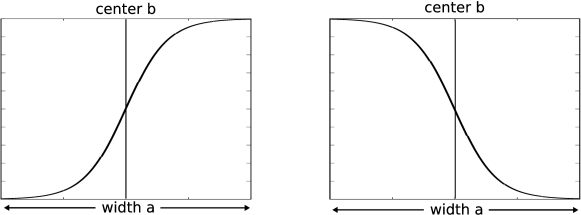
Figure 1: Switching functions: the left switching function is used to guarantee that only one measurement is done at a time point, the right one is used to guarantee that if a perturbation is done at a time point no measurement is done at the same time point.

In literature, problems as (36) fall into the class of semi-infinite inequality and equality constrained optimization problems (SIECP) [38].
Several methods to solve such SIECP problems are available, an overview can be found in [21, 38]. We choose the method of outer approximation [41, 42, 38], whose origin can be traced back to cutting plane methods for convex problems [38]. This approach is beneficial in the presence of a complex inner problem, in our case the robustification against the parameters $\theta_{r_{1}}\mathrm{and}\ \theta_{r_{2}}$. The outer approximation algorithm iteratively solves discretized finite counterparts $\mathbf{P}_{\widetilde{\Theta}^{N}}$ of the semi-infinite problem $\mathbf{P}_{\Theta}$ in each step $N$, successively refining the discretization $\widetilde{\Theta}^{N}$ until a sufficient approximation of the original problem $\mathbf{P}_{\Theta}$ is reached. For problem (36) this means that in each iteration of the outer approximation scheme $\Theta_{r_{1}}$ and $\Theta_{r_{2}}$ are replaced by finite approximations $\widetilde{\Theta}^{N}_{r_{1}}$ and respectively $\widetilde{\Theta}^{N}_{r_{2}}$ with $\widetilde{\Theta}^{N}:=\{(\widetilde{\Theta}^{N}_{r_{1}},\widetilde{\Theta}^{N}_{r_{2}})|r_{j}\in\{1,...,M_{j}\}\}$. This relation between the semi-infinite problem and an infinite sequence of finite problems can be formalized in the theory of consistent approximations and epi-convergence [35, 36, 37, 38].

We use a modified version of Algorithm 3.6.4 in [38] where “Step 1.”, the calculation of augmenting vectors $\tilde{\theta}^{N+1}_{r_{1}}$ and $\tilde{\theta}^{N+1}_{r_{1}}$ to construct

$$\widetilde{\Theta}^{N+1}_{r_{1}}:=\{\tilde{\theta}^{N+1}_{r_{1}}\}\cup\widetilde{\Theta}^{N}_{r_{1}}\quad\mathrm{and}\quad\widetilde{\Theta}^{N+1}_{r_{2}}:=\{\tilde{\theta}^{N+1}_{r_{2}}\}\cup\widetilde{\Theta}^{N}_{r_{2}},$$ (38)

is realized by

$$(\tilde{\theta}^{N+1}_{r_{1}},\tilde{\theta}^{N+1}_{r_{2}}):=arg\min_{\begin{subarray}{c}\theta_{r_{1}}\in\Theta_{r_{2}}\\ \theta_{r_{2}}\in\Theta_{r_{2}}\end{subarray}}\mathcal{I}(P_{r_{2}}(\theta_{r_{2}}):P_{r_{1}}(\theta_{r_{1}}),\mathcal{O}_{1};\xi_{N}),$$ (39)

with $\xi_{N}$ denoting a locally optimal design of the previous problem $\mathbf{P}_{\widetilde{\Theta}^{N}}$. The algorithmic scheme is as follows:

Algorithm 1.

 

• Data. Choose $\xi_{0}\in\Xi$ and a sequence $\{\epsilon_{N}\}^{\infty}_{N=1}$ with $\epsilon_{N}>0$ and $\epsilon_{N}\downarrow 0$.

• Step 0. Set $N=1$, set $\widetilde{\Theta}_{r_{j}}^{0}:=\emptyset$.

• Step 1. Calculate $\widetilde{\Theta}^{N}$ according to (38) and (39).

• Step 2. Calculate approximate solution of $\mathbf{P}_{\widetilde{\Theta}^{N}}$ such that

  $${\color[rgb]{0,0,0}\Psi}_{\widetilde{\Theta}_{N}}((\tau_{N},\xi_{N}))\geq-\epsilon_{N},$$ (40)

  and the equality and inequality constraints in problem $\mathbf{P}_{\widetilde{\Theta}^{N}}$ are fulfilled up to $\epsilon_{N}$.

• Step 3. Replace $N$ by $N+1$, and goto Step 1.

 

${\color[rgb]{0,0,0}\Psi}_{\widetilde{\Theta}_{N}}(\cdot):\mathbb{R}^{d+1}\rightarrow\mathbb{R}_{\leq 0}$ denotes the optimality function associated to problem $\mathbf{P}_{\widetilde{\Theta}^{N}}$, see Theorem 2.2.24 in [38]. The optimality function ${\color[rgb]{0,0,0}\Psi}_{\widetilde{\Theta}_{N}}(\cdot)$ is always non positive and directly related to the first order generalized Karush-Kuhn-Tucker (KKT) conditions, i.e. ${\color[rgb]{0,0,0}\Psi}_{\widetilde{\Theta}_{N}}((\tau,\xi))=0$ if evaluated at a generalized KKT point, see Theorem 2.2.19 in [38].
Assuming that $\mathcal{I}(P_{r_{2}}(\theta_{r_{2}}):P_{r_{1}}(\theta_{r_{1}}),\mathcal{O}_{1};\xi)$ and $\nabla_{\xi}\mathcal{I}(P_{r_{2}}(\theta_{r_{2}}):P_{r_{1}}(\theta_{r_{1}}),\mathcal{O}_{1};\xi)$ are Lipschitz continuous on bounded sets with respect to $\xi$ and $\theta_{r_{j}}$ and $\Theta_{r_{j}}$ are compact any accumulation point of Algorithm 1 fulfills the generalized KKT conditions, compare Theorem 3.6.5 in [38].

To calculate $\tilde{\theta}^{N+1}_{r_{j}}$ in Step 1. of Algorithm 1 we use on heuristic base a simple random search approach coupled to a local optimization method, i.e. we have randomly generated $P$ different start values in $\Theta_{r_{j}}$, from which we have started the local optimization method for parameter estimation. The best value out of the $P$ trials is chosen to augment the set $\widetilde{\Theta}^{N}_{r_{j}}$. Of course there are more sophisticated approaches to search for a global minimum for a review see e.g. [4], but at this point an effective calculation of Step 1. of Algorithm 1 was not our primary goal. For the local parameter optimization we use the same optimization method as for Step 2. in Algorithm 1.

In our implementation we use a fixed $\epsilon$ at the desired final accuracy to solve problem $\mathbf{P}_{\widetilde{\Theta}^{N}}$ in every loop of Step 2. of Algorithm 1, i.e. $\epsilon_{N}=\epsilon$, $N>0$. In that way Step 1. of Algorithm 1 gives a worst case estimate of the KL divergence $\mathcal{I}(P_{r_{2}}(\theta_{r_{2}}):P_{r_{1}}(\theta_{r_{1}}),\mathcal{O}_{1};\xi_{N})$ for the current design $\xi_{N}$ with respect to $\theta_{r_{j}}$. Therefore for practical application the algorithm can be stopped if the worst case estimate of KL divergence for the current design $\xi_{N}$ is big enough although no local optima might be achieved during optimization. As stopping criterion of Algorithm 1 we use:

Algorithmic Stop Criterion.

Stop after Step 1. of Algorithm 1, if

$$\begin{split}\delta\geq&{\color[rgb]{0,0,0}\min_{\begin{subarray}{\ }r_{1}\in\{1,...,M_{1}\}\\ r_{2}\in\{1,...,M_{2}\}\end{subarray}}}\min_{\begin{subarray}{c}\theta_{r_{1}}\in\widetilde{\Theta}^{N-1}_{r_{1}}\\ \theta_{r_{2}}\in\widetilde{\Theta}^{N-1}_{r_{2}}\end{subarray}}\mathcal{I}(P_{r_{2}}(\theta_{r_{2}}):P_{r_{1}}(\theta_{r_{1}}),\mathcal{O}_{1};\xi_{N-1})-\\ &{\color[rgb]{0,0,0}\min_{\begin{subarray}{\ }r_{1}\in\{1,...,M_{1}\}\\ r_{2}\in\{1,...,M_{2}\}\end{subarray}}}\min_{\begin{subarray}{c}\theta_{r_{1}}\in\Theta_{r_{1}}\\ \theta_{r_{2}}\in\Theta_{r_{2}}\end{subarray}}\mathcal{I}(P_{r_{2}}(\theta_{r_{2}}):P_{r_{1}}(\theta_{r_{1}}),\mathcal{O}_{1};\xi_{N-1})=:\Delta_{RG},\end{split}$$ (41)

where $\delta$ is a small positive constant, then consider $(\tilde{\theta}^{N+1}_{r_{1}},\tilde{\theta}^{N+1}_{r_{2}})$, $r_{1}\in\{1,...,M_{1}\}$, $r_{2}\in\{1,...,M_{2}\}$ and $\xi_{N}$ as (approximate) solutions of problem $\mathbf{P}_{\Theta}$, else goto Step 2. and calculate a new design $\xi_{N+1}$.

This stop criterion has also been used in [42, 39]. We call the distance $\Delta_{RG}$ given by (41), robustification gap.

3.1 Numerical solution of the problem $\mathbf{P}_{\widetilde{\Theta}^{N}}$

We have implemented the resulting optimization problem in a multiple shooting setup (see for example [45, 14, 13]). In our multiple shooting setup the whole integration interval $[0,T_{\mathrm{end}}]$ is subdivided into several subintervals by introducing auxiliary multiple shooting node variables $s_{{r_{j}},i,l}$, $j\in\{1,2\},\ r_{j}\in\{1,...,M_{j}\},\ i\in\{1,...,n\},\ l\in\{1,...,N\}$, on each of which an independent initial value problem is solved. Each end point of a subinterval corresponds to one measurement time point. Matching conditions which enter the optimization problem as additional equality constraints assure continuity of the state trajectory from one subinterval to the next.

To incorporate the perturbations $c$ matching conditions

$$s_{r_{j},i,l}-y_{r_{j}}(t_{i-1},t_{i},s_{r_{j},i-1,l},\tilde{\theta}_{r_{j}}^{l})=0,$$ (42)

$s_{r_{j},i,l}$, denoting the multiple shooting nodes with $s_{r_{j},0,l}=y_{I}$ are modified to

$$\begin{split}s_{r_{j},i,l}-y_{r_{j}}(t_{i-1},t_{i},s_{j,i-1,l},\tilde{\theta}_{r_{j}}^{l})=c_{i},&\quad i\in\{1,...,n-1\},\\ s_{r_{j},n,l}-y_{r_{j}}(t_{n-1},t_{n},s_{j,n-1,l},\tilde{\theta}_{r_{j}}^{l})=0.\end{split}$$ (43)

A graphical scheme of the multiple shooting setup is shown in Figure 2.
Instead of evaluating the objective functional (35) by use of the values $y_{r_{j}}^{i}$, given by the solution of the initial value problem (11), depending on the parameters $\tilde{\theta}_{r_{j}}$, (35) is evaluated by use of the auxiliary multiple shooting node variables $s_{r_{j},i,l}$ replacing the values $y_{r_{j}}^{i}$ with $s_{r_{j},i,l}$ respectively. The dependency of (35) on $s_{r_{j},i,l}$ is indicated by $\mathcal{I}(s_{r_{1},\cdot,l},s_{r_{2},\cdot,l})$.

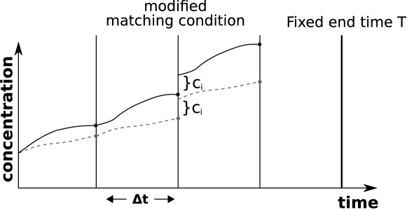
Figure 2: Scheme of the multiple shooting setup for computing the experimental design to discriminate two models. A dot denotes one measurement time point. The black solid line corresponds to model 1 and the gray dashed one to model 2.

The overall optimization problem can be stated as

$$\max_{\tau,y_{I},\Delta t,c,s}\tau$$ (44)

subject to

$$\begin{array}[]{c}\frac{\mathrm{d}y_{r_{j}}}{\mathrm{d}\mathfrak{t}}=f^{\mathrm{rhs}}_{r_{j}}(y,\tilde{\theta}_{r_{j}}^{l}),\quad\mathfrak{t}\in[t_{i-1},t_{i}],\quad y_{r_{j}}(t_{i-1}):=s_{r_{j},i-1,l}\\ s_{r_{j},i,l}-y_{r_{j}}(t_{i-1},t_{i},s_{r_{j},i-1,l},\tilde{\theta}_{r_{j}}^{l})=c_{i},\\ s_{r_{j},n,l}-y_{r_{j}}(t_{n-1},t_{n},s_{r_{j},n-1,l},\tilde{\theta}_{r_{j}}^{l})=0,\\ s_{r_{j},0,l}=y_{I},\\ y_{I}^{\mathrm{min}}\leq y_{I}\leq y_{I}^{\mathrm{max}},\\ 0\leq\Delta t\leq t^{\mathrm{max}},\\ 0\leq c\leq c^{\mathrm{max}},\\ s_{r_{j},i,l}^{\mathrm{min}}\leq s_{r_{j},i,l}\leq s_{r_{j},i,l}^{\mathrm{max}},\\ \sum_{i=1}^{n}\Delta t_{i}=T_{\mathrm{end}},\\ \mathcal{I}(s_{r_{1},\cdot,l},s_{r_{2},\cdot,l})-\tau\geq 0,\ r_{1}\in\{1,...,M_{1}\},\ r_{2}\in\{1,...,M_{2}\},\end{array}$$ (45)

with $j\in\{1,2\},\ r_{j}\in\{1,...,M_{j}\},\ i\in\{1,...,n\},\ l\in\{1,...,N\}$.

We have implemented this problem within the interior point optimization package IPOPT [50, 51], using the linear solver MA27 [23]. Usually for the solution of the KKT system within the direct multiple shooting ansatz the linear system is solved utilizing tailored structure-exploitation, e.g., condensing or high rank updates. See for example [30]. Since speed aspects are not our primary concern we rely on the sparse solver MA27 instead of developing a tailored solver for this problem class at the current stage.
All derivatives up to second order, which are used for the calculations of the Hessian needed for a robust performance of IPOPT, are calculated by automatic differentiation using CppAD, [9, 8].
For the solution of the differential equations within the optimization problem, which are commonly stiff in chemical and biochemical applications, we have implemented a fully variable step, variable order (order $1$ to $6$), Backward differentiation formulae (BDF) method, based on Nordsiek array polynomial interpolation similar to the EPISODE BDF method by Byrne and Hindmarsh [16], but with the step size selection strategy of Calvo and Rández [17].
For the generation of sensitivities we have adopted the sophisticated principles of internal numerical differentiation developed by Albersmeyer and Bock [2, 1] in forward and adjoint mode.
The idea of this principle is instead of calculating the sensitivities by use of the sensitivity differential equation, to directly differentiate the BDF integration scheme by automatic differentiation, which we implemented using CppAD [9, 8].
According to some notes in the PhD thesis of Albersmeyer [1] we also have implemented the possibility to control the step size scheme not only by the local truncation error of the nominal trajectory but as well by the local truncation error of the sensitivities generated by the forward mode of automatic differentiation with respect to the sensitivity differential equation, which has shown by numerical experience to improve the robustness of the optimization approach.
A different approach would be to use collocation, i.e. to incorporate a full discretization of the ODEs into the optimization problem, see e.g. [11]. Since the kinetic ODE systems in the focus of our applications are usually stiff, we prefer adaptive time integration.

3.2 Stabilizing homotopy method for subsequent $\mathbf{P}_{\widetilde{\Theta}^{N+1}}$

By solving the subsequent optimization problems $\mathbf{P}_{\widetilde{\Theta}^{N+1}}$ with an interior point code like IPOPT [50, 51] initialized with primal and dual variables of the previous problem or with primal variables only, one often observes that the new solution may differ significantly from the previous. This is due to the fact that the solution of the previous problem $\mathbf{P}_{\widetilde{\Theta}^{N}}$ is infeasible for $\mathbf{P}_{\widetilde{\Theta}^{N+1}}$ and thus the algorithm tries to find a feasible state before it proceeds to find a new optimum. This behavior is not desired in the context of an outer approximation algorithm, because convergence of the algorithm may be slowed down significantly. This circumstance originates from a jumping between vicinities of distinct local maxima of problem (36). The discretization $\widetilde{\Theta}^{N}$ of the robustification space may not be equally adequate for different local maxima. To overcome this problem we have implemented a heuristic homotopy method to gradually introduce the additional constraints

$$g_{r_{1},r_{2}}(\tau,\xi)_{N+1}:=\mathcal{I}(s_{r_{1},\cdot,N+1},s_{r_{2},\cdot,N+1})-\tau\geq 0,$$ (46)

of problem $\mathbf{P}_{\widetilde{\Theta}^{N+1}}$. We replace $g_{r_{1},r_{2}}(\tau,\xi)_{N+1}$ by

$$\tilde{g}_{r_{1},r_{2}}(\tau,\xi;\kappa)_{N+1}:=\mathcal{I}(s_{r_{1},\cdot,N+1},s_{r_{2},\cdot,N+1})-\tau+(1-\kappa)\rho\geq 0,$$ (47)

with homotopy parameter $\kappa\in[0,1]$ and $\rho$ is a constant which has to be set such that $\tilde{g}_{r_{1},r_{2}}(\tau,\xi;\kappa)_{N+1}$ are inactive for $\kappa=0$ at the initial design $\xi_{N}$. We choose $\rho$ to be

$$\begin{split}\rho:=K\cdot\max_{\begin{subarray}{c}r_{1}\in\{1,...,M_{1}\}\\ r_{2}\in\{1,...,M_{2}\}\end{subarray}}&\left(\min_{\begin{subarray}{c}\theta_{r_{1}}\in\widetilde{\Theta}^{N}_{r_{1}}\\ \theta_{r_{2}}\in\widetilde{\Theta}^{N}_{r_{2}}\end{subarray}}\mathcal{I}(P_{r_{2}}(\theta_{r_{2}}):P_{r_{1}}(\theta_{r_{1}}),\mathcal{O}_{1};\xi_{N})-\right.\\ &\ \ \ \left.\min_{\begin{subarray}{c}\theta_{r_{1}}\in\Theta_{r_{1}}\\ \theta_{r_{2}}\in\Theta_{r_{2}}\end{subarray}}\mathcal{I}(P_{r_{2}}(\theta_{r_{2}}):P_{r_{1}}(\theta_{r_{1}}),\mathcal{O}_{1};\xi_{N})\right).\end{split}$$ (48)

$K$ is a save guard factor we set empirically to $K=1.4$, which worked well in practice for our examples. For $\kappa=0$ the augmented optimization problem should be easily solvable within a few iterations by performing a warm start from the solution of the previous problem. By increasing the homotopy parameter to $\kappa=1$ the additional constraint is gradually introduced, which leads to a sequence of easily solvable subproblems whose solutions stay in the vicinity of the solution of the previous problem $\mathbf{P}_{\widetilde{\Theta}^{N}}$. A similar homotopy strategy can be found e.g. in [40].

4 Numerical results

We have applied the algorithm developed in Section 2 and 3 to two example problems for which we present results in the following section. For the purpose of illustration we restrict ourself to the case that each hypothesis comprise only one model whereby we assume that only the alternative hypothesis is composite. We also assume that each species is “directly” measurable. We treat model 1 as null hypothesis and model 2 as alternative hypothesis.

4.1 Discriminating design for two models describing glycolytic oscillations

In the first test case for model discrimination we implemented the following models for glycolytic oscillations as described in [20].

Model 1 is an allosteric enzyme model with positive feedback under cooperativity and linear product sink. The differential equations for model 1 are given by

$$\begin{split}\dfrac{d\alpha_{1}}{dt}&=\nu-\sigma\phi(\alpha_{1},\gamma_{1}),\\ \dfrac{d\gamma_{1}}{dt}&=q_{1}\sigma\phi(\alpha_{1},\gamma_{1})-k_{s}\gamma_{1},\\ \phi(\alpha_{1},\gamma_{1})&=\dfrac{\alpha_{1}(1+\alpha_{1})(1+\gamma_{1})^{2}}{L_{1}+(1+\alpha_{1})^{2}(1+\gamma_{1})^{2}}.\end{split}$$

Model 2 is an allosteric model with positive feedback in the absence of cooperativity and the product sink is represented by Michaelis-Menten kinetics. The differential equations for Model 2 are given by

$$\begin{split}\dfrac{d\alpha_{2}}{dt}&=\nu-\phi(\alpha_{2},\gamma_{2}),\\ \dfrac{d\gamma_{2}}{dt}&=q_{2}\phi(\alpha_{2},\gamma_{2})-\dfrac{r_{s}\gamma_{2}}{\mu+\gamma_{2}},\\ \phi(\alpha_{2},\gamma_{2})&=\dfrac{\alpha_{2}(1+\gamma_{2})}{L_{2}+(1+\alpha_{2})(1+\gamma_{2})}.\end{split}$$

$\alpha_{1,2}$ denotes the species concentration of the substrate $\gamma_{1,2}$ that of the product.
For both models the inflow parameter $\nu$ is the same and fixed to the value $\nu=0.22$. It represents the inflow of substrate to the experimental system, a CSTR (continuously stirred tank reactor).
The parameters $\sigma$, $q_{1}$, $k_{s}$ and $L_{1}$ of model 1 are regarded as known. Their values are given in Table 1, the parameters $q_{2}$, $r_{s}$, $\mu$ and $L_{2}$ of model 2 are regarded as unknown and subject to robustification. For the permitted parameter range see Table 1.

Model 1				Model 2
$\sigma$	$q_{1}$	$k_{s}$	$L_{1}$	$q_{2}$	$r_{s}$	$\mu$	$L_{2}$
0.92	2.01	0.11	17206.10	$[10^{-7},100]$	$[10^{-7},100]$	$[10^{-7},100]$	$[100,300]$

Table 1: Parameter values for the glycolytic oscillation models.

For simplicity we consider the homoscedastic case with equal variances, i.e. $v_{1}=v_{2}=\sigma^{2}$. In this case $\mathcal{I}(P_{1}:P_{2},\mathcal{O}_{1})$ reduces to,

$$\mathcal{I}(P_{1}:P_{2},\mathcal{O}_{1})=\sum_{i=1}^{n}{\color[rgb]{0,0,0}\mathcal{H}^{\prime}}(t_{i}){\color[rgb]{0,0,0}\widetilde{\mathcal{H}^{\prime}}}(c_{i})\left((\alpha^{i}_{1}-\alpha^{i}_{2})^{2}+(\gamma^{i}_{1}-\gamma^{i}_{2})^{2}\right).$$ (49)

For this test case the homotopy strategy as presented in Section 3.2 is only applied if the robustification gap $\Delta_{RG}<0.1$, then the successive problem $\mathbf{P}_{\widetilde{\Theta}^{N+1}}$ is calculated by use of the homotopy strategy with $30$ homotopy steps, i.e. $\kappa_{h}=h/30$, $h\in\{1,...,30\}$. Otherwise the problem $\mathbf{P}_{\widetilde{\Theta}^{N+1}}$ is solved without homotopy strategy. For each subsequent problem $\mathbf{P}_{\widetilde{\Theta}^{N+1}}$ the solution of problem $\mathbf{P}_{\widetilde{\Theta}^{N}}$ is used as initial guess.

We first present a robust design without the possibility to disturb the system by adding species at later time points.
The design is calculated within a fixed time window i.e. $T_{\mathrm{end}}=400$. $100$ equally spaced possible measurement points are defined in the initial state of the optimization procedure, the distance vector $\Delta t$ between the time points is subject to design and each entry is restricted to $\Delta t_{i}\in[10^{-7},10^{19}],$ $i\in\{1,...,100\}$. The disturbance vectors $c_{i}$ are set to $c_{i}=0$, $i\in\{1,...,99\}$ and are fixed to model the fact that no species disturbance is allowed.
The initial species concentrations which are also subject to experimental design are restricted to $\alpha_{I}\in[10^{-7},25]$ and $\gamma_{I}\in[10^{-7},25]$. The initial values were set to $\alpha_{I}=15$ and $\gamma_{I}=2$. The parameters of the switching functions ${\color[rgb]{0,0,0}\mathcal{H}^{\prime}}(t_{i})$ are chosen as $a_{1}=20.0$ and $b_{1}=10.0$. The parameters of the switching functions ${\color[rgb]{0,0,0}\widetilde{\mathcal{H}^{\prime}}}(c_{i})$ are chosen as $a_{2}=0.05$ and $b_{2}=0.025$. The algorithmic settings are summarized in Table 2.

Optimization settings			Integrator settings
$P$	$\delta$	IPOPT-tol: Step 1./Step 2.	relTol/absTol	relTolSens/absTolSens
$5$	$10^{-6}$	$10^{-10}$/$10^{-8}$	$10^{-12}$/$10^{-12}$	$10^{-12}$/$10^{-12}$

Table 2: On the left hand side the optimization settings are listed comprising the IPOPT stopping tolerances for Step 1. and Step 2. of Algorithm 1 and on the right hand side the integration tolerances for the nominal trajectory and the first order sensitivities. We use the IPOPT option “honor_original_bounds=no” for Step 1. and Step 2. of Algorithm 1.

A plot of the functions $\alpha_{1},\alpha_{2}$ and $\gamma_{1},\gamma_{2}$ in the initial state and for the solution of problem $\mathbf{P}_{\widetilde{\Theta}^{1}}$ are shown in Figure 3. A plot for the same functions with the same solution design as for problem $\mathbf{P}_{\widetilde{\Theta}^{1}}$ after the next robustification step is shown in Figure 4. The final design is also shown in Figure 4.

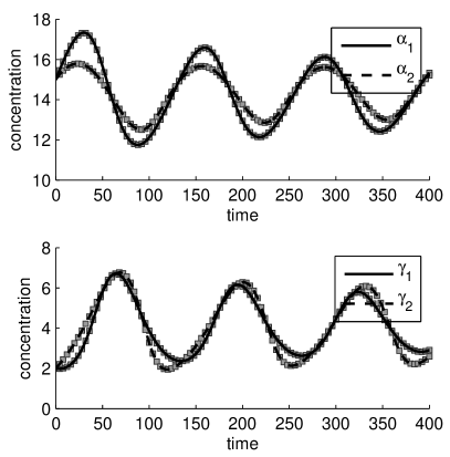
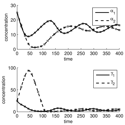
Figure 3: The model functions $\alpha_{1},\alpha_{2}$ and $\gamma_{1},\gamma_{2}$ are shown before the optimization procedure (left) and after the optimization procedure of problem $\mathbf{P}_{\widetilde{\Theta}^{1}}$ (right) for the glycolytic design setup without the possibility to disturb the system. One square represents one measurement time point.

A plot of the robustification gap $\Delta_{RG}$ and as well for the objective value of problem $\mathbf{P}_{\widetilde{\Theta}^{N}}$ for each iteration $N$ of Algorithm 1 are shown in Figure 5. A selection of design variables as solutions of problem $\mathbf{P}_{\widetilde{\Theta}^{N}}$ is shown in Figure 6(left).

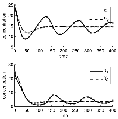
Figure 4: The model functions $\alpha_{1},\alpha_{2}$ and $\gamma_{1},\gamma_{2}$ are shown for the same solution design as for problem $\mathbf{P}_{\widetilde{\Theta}^{1}}$ after the next robustification step (left) and for the final design (right) for the glycolytic design setup without the possibility to disturb the system. One square represents one measurement time point.

\psfrag{label1}{\parbox{113.81102pt}{\mbox{} \\ \mbox{} \\ $N$}}\psfrag{label2}{\parbox{113.81102pt}{\vspace{-0.3cm} $\Delta_{RG}$}}\includegraphics[width=195.12767pt]{./PLOT_ROBUSTIFIKATION_GAP_GNPD.eps}

\psfrag{label1}{\parbox{113.81102pt}{\mbox{} \\ \mbox{} \\ $N$}}\psfrag{label2}{\parbox{113.81102pt}{\vspace{-0.3cm} $\Delta_{RG}$}}\psfrag{label2}{\parbox{113.81102pt}{\vspace{-0.3cm} objective value of $\mathbf{P}_{\widetilde{\Theta}_{N}}$}}\includegraphics[width=195.12767pt]{./PLOT_OBJECTIVE_GNPD.eps}

Figure 5: In the left figure the robustification gap $\Delta_{RG}$ is plotted versus the number of iterations $N$ of Algorithm 1 and in the right figure the objective value of problem $\mathbf{P}_{\widetilde{\Theta}^{N}}$ is shown for the glycolytic design setup without the possibility to disturb the system.

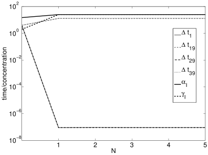
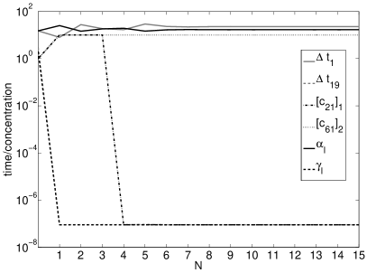
Figure 6: A selection of design variables as solutions of problem $\mathbf{P}_{\widetilde{\Theta}^{N}}$ for the glycolytic design setup without the possibility to disturb the system (left) and with the possibility to disturb the system (rigth) are shown.

In a second scenario we additionally allow for species perturbations. In this new scenario at the $21$th $41$th, $61$th and $81$th measurement time points, the system can get disturbed by additional species quantities. The free vectors $c_{i}$, $i\in\{21,41,61,81\}$ are constrained by $c_{i}\in[10^{-7},10]$. The initial values are set to $c_{i}=1$. The remaining conditions are as before, however we change the time vector bound constraints for $i\in\{1,6,11,21,26,31,41,46,51,61,66,71,81\}$ to $\Delta t_{i}\in[8,10^{19}]$ and the initial state to $\Delta t_{i}=15$. The bounds for the remaining entries are as before, and the remaining measurement time points were equally spaced.
A plot of the functions $\alpha_{1},\alpha_{2}$ and $\gamma_{1},\gamma_{2}$ in the initial state and for the solution of problem $\mathbf{P}_{\widetilde{\Theta}^{1}}$ are shown in Figure 7. A plot for the same functions with the same solution design as for problem $\mathbf{P}_{\widetilde{\Theta}^{1}}$ after the next robustification step is shown in Figure 8. The final design is also shown in Figure 8.

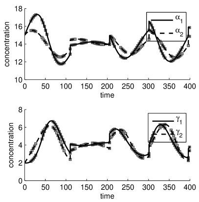
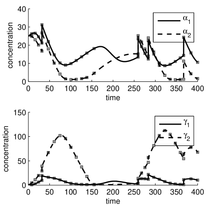
Figure 7: The model functions $\alpha_{1},\alpha_{2}$ and $\gamma_{1},\gamma_{2}$ are shown before the optimization procedure (left) and after the optimization procedure of problem $\mathbf{P}_{\widetilde{\Theta}^{1}}$ (right) for the glycolytic design setup with the possibility to disturb the system. One square represents one measurement time point.

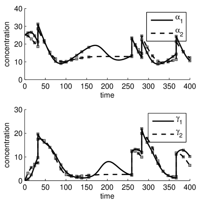
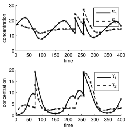
Figure 8: The model functions $\alpha_{1},\alpha_{2}$ and $\gamma_{1},\gamma_{2}$ are shown for the same solution design as for problem $\mathbf{P}_{\widetilde{\Theta}^{1}}$ after the next robustification step (left) and for the final design (right) for the glycolytic design setup with the possibility to disturb the system. One square represents one measurement time point.

A plot of the robustification gap $\Delta_{RG}$ and the objective value of problem $\mathbf{P}_{\widetilde{\Theta}^{N}}$ for each iteration $N$ of Algorithm 1 are shown in Figure 9. A selection of design variables as solutions of problem $\mathbf{P}_{\widetilde{\Theta}^{N}}$ is shown in Figure 6(right).

\psfrag{label1}{\parbox{113.81102pt}{\mbox{} \\ \mbox{} \\ $N$}}\psfrag{label2}{\parbox{113.81102pt}{\vspace{-0.3cm} $\Delta_{RG}$}}\includegraphics[width=195.12767pt]{./PLOT_ROBUSTIFIKATION_GAP_GYPD.eps}

\psfrag{label1}{\parbox{113.81102pt}{\mbox{} \\ \mbox{} \\ $N$}}\psfrag{label2}{\parbox{113.81102pt}{\vspace{-0.3cm} $\Delta_{RG}$}}\psfrag{label2}{\parbox{113.81102pt}{\vspace{-0.3cm} objective value of $\mathbf{P}_{\widetilde{\Theta}_{N}}$}}\includegraphics[width=195.12767pt]{./PLOT_OBJECTIVE_GYPD.eps}

Figure 9: In the left figure the robustification gap $\Delta_{RG}$ is plotted versus the number of iterations $N$ of Algorithm 1 and in the right figure the objective value of problem $\mathbf{P}_{\widetilde{\Theta}^{N}}$ is shown for the glycolytic design setup with the possibility to disturb the system.

4.2 Discriminating design for two models describing signal sensing in dictyostelium discoideum

The second test case is the discrimination of two models describing the chemotactic response in the amoeba Dictyostelium discoideum as presented in [33] using the framework presented in Section 2 and 3. The two models describe the adaption mechanism observed when amoebae encounter the chemoattractant cAMP [31], see figure 10.

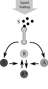
(a) model 1

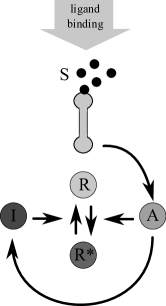
(b) model 2

Figure 10: Two models of the signal system of the Dictyostelium amoeba.

For both models, a chemotaxis response regulator $R$ gets activated ($R^{*}$) by an activator enzyme $A$, when a cAMP ligand $S$ appears. But the deactivating mechanism determined by the interaction with an inhibitor molecule $I$ differs for both models. Both models comprise mass action kinetics in form of ODE.

In model 1 the activator enzyme as well as the inhibitor enzyme are regulated by the external signal , which is proportional to the cAMP concentration $S$. The overall model in this case is given by,

$$\begin{split}\dot{A}_{1}&=-k_{-a}A_{1}+k_{a}S_{1}\\ \dot{I}_{1}&=-k_{-i}I_{1}+k_{i_{1}}S_{1}\\ \dot{R}_{1}^{*}&=-(k_{r}A_{1}+k_{-r}I_{1})R_{1}^{*}+k_{r}R_{T}A_{1},\end{split}$$ (50)

where $k_{-a}$, $k_{a}$, $k_{-i}$, $k_{i_{1}}$, $k_{r}$ and $k_{-r}$ are the mass action rate constants and $R_{T}:=R^{*}+R$ is the total amount of the response regulator.

In model 2 the inhibitory molecule $I$ is activated through the indirect action of activator $A$ instead of direct activation by sensing ligand binding. The overall model in this case is given by,

$$\begin{split}\dot{A}_{2}&=-k_{-a}A_{2}+k_{a}S_{2}\\ \dot{I}_{2}&=-k_{-i}I_{2}+k_{i_{2}}A_{2}\\ \dot{R}_{2}^{*}&=-(k_{r}A_{2}+k_{-r}I_{2})R_{2}^{*}+k_{r}R_{T}A_{2},\end{split}$$ (51)

where $k_{-a}$, $k_{a}$, $k_{-i}$, $k_{i_{2}}$, $k_{r}$ and $k_{-r}$ are the mass action rate constants and $R_{T}:=R^{*}+R$ is the total amount of the response regulator.
For modeling details we refer to [33]. We have extended these systems of ordinary differential equations by an additional state corresponding to the cAMP ligand $S$ with $\dot{S}=0$. By allowing species concentration perturbations $c$ only to the state $S$ we can mimic a piecewise constant control of the system by the cAMP ligand $S$.

The experimental design parameters are the initial species concentrations of the four states namely, $A_{I}$, $I_{I}$, $R_{I}$, $S_{I}$, the measurement time points $t$ and the species concentration perturbation $c$ with respect to S. We discard the condition that either a measurement or a perturbation can be performed since in that setting by use of the perturbations $c$ we mimic a piecewise constant input control $S$ and therefore that restriction seems unnatural. Again for simplicity we consider the homoscedastic case with equal variances i.e. $v_{1}=v_{2}=\sigma^{2}$, where $\mathcal{I}(P_{1}:P_{2},\mathcal{O}_{1})$ reduces now to

$$\mathcal{I}(P_{1}:P_{2},\mathcal{O}_{1})=\sum_{i=1}^{n}{\color[rgb]{0,0,0}\mathcal{H}^{\prime}}(t_{i})\left((A^{i}_{1}-A^{i}_{2})^{2}+(I^{i}_{1}-I^{i}_{2})^{2}+(R^{*,i}_{1}-R^{*,i}_{2})^{2}\right).$$ (52)

The parameters $k_{-a}$, $k_{a}$, $k_{-i}$, $k_{i_{1}}$, $k_{r}$, $k_{-r}$ and $R_{T}$ are regarded as known and fixed, their values are given in Table 3.

$k_{-a}$	$k_{a}$	$k_{-i}$	$k_{i_{1}}$	$k_{r}$	$k_{-r}$	$R_{T}$
2.0	3.0	0.1	1.0	1.0	1.0	23/30

Table 3: Parameter values for the fix values within model 1 and model 2.

Parameter $k_{i_{2}}$ is regarded as unknown and subject to robustification. The range of the parameter $k_{i_{2}}$ is set to $k_{i_{2}}\in[0,2]$.
The optimal design is calculated within a fixed time window with $T_{\mathrm{end}}=100$. $100$ equally spaced possible measurement points are defined in the initial state of the optimization procedure. The distance vector $\Delta t$ between time points is subject to design and each entry is restricted to $\Delta t_{i}\in[10^{-7},10^{19}],$ $i\in\{1,...,100\}$.
The free perturbation vectors $c_{i}$, $i\in\{11,21,31,41,51,61,71,81,91\}$ are not restricted. The initial values are set to $c_{i}=0$, $i\in\{11,21\}$, $c_{31}=0.3$, $c_{i}=-0.48$, $i\in\{41,61,81\}$ and $c_{i}=0.48$, $i\in\{51,71,91\}$.
The initial species concentrations which are also subject to the experimental design are restricted to $S_{I}\in[0.01,0.5]$, $A_{I}\in[10^{-7},1]$, $I_{I}\in[10^{-7},1]$ and $R_{I}\in[10^{-7},I]$. The initial values are set to $S_{I}=0.2$, $A_{I}=1.0$, $I=10^{-4}$ and $R=10^{-4}$. The multiple shooting intermediate variables for the species $S$ are restricted to $s_{i}\in[0.01,0.5]$ to restrict the piecewise constant control to this interval. The parameters of the switching functions ${\color[rgb]{0,0,0}\mathcal{H}^{\prime}}(t_{i})$ are chosen as $a_{1}=5.0$ and $b_{1}=2.5$. The algorithmic settings are summarized in Table 4.

Optimization settings			Integrator settings
$P$	$\delta$	IPOPT-tol: Step 1./Step 2.	relTol/absTol	relTolSens/absTolSens
$5$	$10^{-8}$	$10^{-10}$/$10^{-11}$	$10^{-14}$/$10^{-14}$	$10^{-14}$/$10^{-14}$

Table 4: On the left hand side the optimization settings are listed comprising the IPOPT stopping tolerances for Step 1. and Step 2. of Algorithm 1 and on the right hand side the integration tolerances for the nominal trajectory and the first order sensitivities. We use the IPOPT option “honor_original_bounds=no” for Step 1. and Step 2. of Algorithm 1.

With these design conditions we start the optimization procedure twice. First by use of the homotopy strategy for successive problems $\mathbf{P}_{\widetilde{\Theta}^{N+1}}$ with $10$ homotopy steps.
Since the “discriminating power” of the experimental setup is very low in this case, i.e. the deviation between the two models is small, we plot the distance functions $(S_{1}-S_{2})$, $(A_{1}-A_{2})$, $(I_{1}-I_{2})$ and $(R_{1}-R_{2})$ for the initial state and for the solution of problem $\mathbf{P}_{\widetilde{\Theta}^{1}}$ in Figure 11. A plot for the same functions with the same solution design as for problem $\mathbf{P}_{\widetilde{\Theta}^{1}}$ after the next robustification step is shown in Figure 12. The final design is also shown in Figure 12.

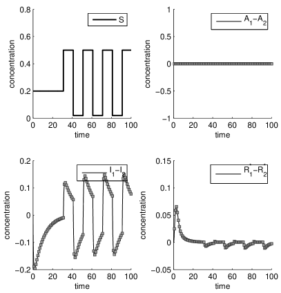
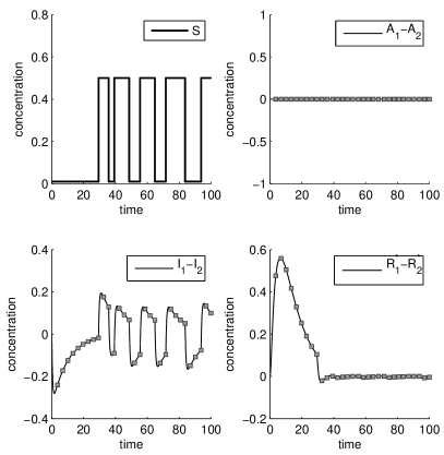
Figure 11: The model variable distance functions $(S_{1}-S_{2})$, $(A_{1}-A_{2})$, $(I_{1}-I_{2})$ and $(R_{1}-R_{2})$ are shown before the optimization procedure (left) and after the optimization procedure of problem $\mathbf{P}_{\widetilde{\Theta}^{1}}$ (right) for two models describing signal sensing in dictyostelium discoideum. One square represents one measurement time point.

A plot of the robustification gap $\Delta_{RG}$ for each iteration $N$ of Algorithm 1 is shown in Figure 13 (left). A plot of the objective value of problem $\mathbf{P}_{\widetilde{\Theta}^{N}}$ for each iteration $N$ of Algorithm 1 is shown in Figure 14 (left). A selection of design variables as solutions of problem $\mathbf{P}_{\widetilde{\Theta}^{N}}$ is shown in Figure 15 (left).

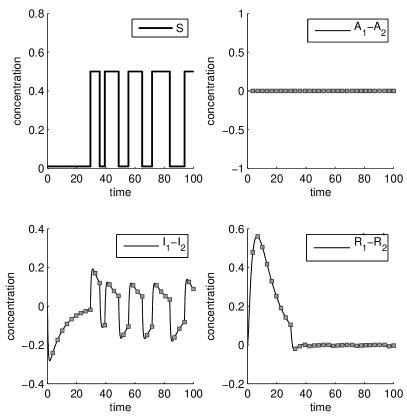
Figure 12: The model variable distance functions $(S_{1}-S_{2})$, $(A_{1}-A_{2})$, $(I_{1}-I_{2})$ and $(R_{1}-R_{2})$ are shown for the same solution design as for problem $\mathbf{P}_{\widetilde{\Theta}^{1}}$ after the next robustification step and for the final design (right) for two models describing signal sensing in dictyostelium discoideum. One square represents one measurement time point.

\psfrag{label1}{\parbox{113.81102pt}{\mbox{} \\ $N$}}\psfrag{label2}{\parbox{113.81102pt}{\vspace{-0.1cm} $\Delta_{RG}$}}\includegraphics[width=212.47617pt]{./PLOT_ROBUSTIFIKATION_GAP_AYPD.eps}

(a) with homotopy strategy

\psfrag{label1}{\parbox{113.81102pt}{\mbox{} \\ $N$}}\psfrag{label2}{\parbox{113.81102pt}{\vspace{-0.1cm} $\Delta_{RG}$}}\includegraphics[width=212.47617pt]{./PLOT_ROBUSTIFIKATION_GAP_AYPDNH.eps}

(b) without homotopy strategy

Figure 13: The robustification gap $\Delta_{RG}$ is plotted versus the number of iterations $N$ of Algorithm 1 for the setup with two models describing signal sensing in dictyostelium discoideum, with homotopy strategy (left) and without homotopy strategy (right).

Second we calculate the design without the homotopy strategy. We experience huge jumps in the final objective value of problem $\mathbf{P}_{\widetilde{\Theta}^{N}}$ for subsequent iterations $N$ of Algorithm 1. This is due to the fact that the final design of the former problem $\mathbf{P}_{\widetilde{\Theta}^{N}}$ is an infeasible starting point for the successive problem $\mathbf{P}_{\widetilde{\Theta}^{N+1}}$ in the interior point solution strategy. First the optimizer tries to force the iterates back into the feasible region and afterwards the new central path leads to a different design.
For this case a plot of the robustification gap $\Delta_{RG}$ for each iteration $N$ of Algorithm 1 is shown in Figure 13 (right). A plot of the objective value of problem $\mathbf{P}_{\widetilde{\Theta}^{N}}$ for each iteration $N$ of Algorithm 1 is shown in Figure 14 (right). A selection of design variables as solutions of problem $\mathbf{P}_{\widetilde{\Theta}^{N}}$ is shown in Figure 15 (right).

\psfrag{label1}{\parbox{113.81102pt}{\mbox{} \\ $N$}}\psfrag{label2}{\parbox{113.81102pt}{\vspace{-0.1cm} objective value of $\mathbf{P}_{\widetilde{\Theta}_{N}}$}}\includegraphics[width=212.47617pt]{./PLOT_OBJECTIVE_AYPD.eps}

(a) with homotopy strategy

\psfrag{label1}{\parbox{113.81102pt}{\mbox{} \\ $N$}}\psfrag{label2}{\parbox{113.81102pt}{\vspace{-0.1cm} objective value of $\mathbf{P}_{\widetilde{\Theta}_{N}}$}}\includegraphics[width=212.47617pt]{./PLOT_OBJECTIVE_AYPDNH.eps}

(b) without homotopy strategy

Figure 14: The objective value of problem $\mathbf{P}_{\widetilde{\Theta}^{N}}$ is plotted versus the number of iterations $N$ of Algorithm 1 for the setup with two models describing signal sensing in dictyostelium discoideum, with homotopy strategy (left) and without homotopy strategy (right).

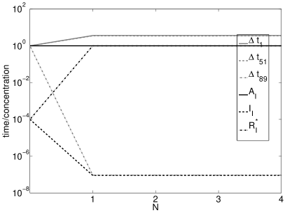
(a) with homotopy strategy

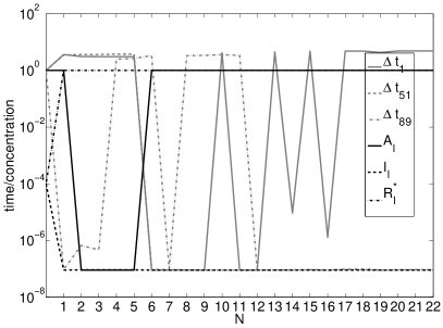
(b) without homotopy strategy

Figure 15: A selection of design variables calculated as solution of problem $\mathbf{P}_{\widetilde{\Theta}^{N}}$ is plotted versus the number of iterations $N$ of Algorithm 1 for the setup with two models describing signal sensing in dictyostelium discoideum, on the left with homotopy strategy and on the right without homotopy strategy.

As one can clearly see, the homotopy strategy helps to considerably stabilize Algorithm 1.

5 Conclusion

We present a framework for the robust computation of optimal experimental designs for the purpose of model discrimination. The theoretical framework as well as the numerical realization by utilization of an outer approximation algorithm are worked out. A strategy for the numerical stabilization of the algorithm by use of a homotopy approach is suggested. The optimization procedure is successfully exemplified on two biological model systems. In our examples we clearly found that the homotopy approach is significantly superior to a cold start of successive design problems $\mathbf{P}_{\widetilde{\Theta}^{N+1}}$. For the first test case, the discrimination of two models describing glycolytic oscillations, the outer approximation scheme completely fails to reach the desired accuracy $\delta$ without homotopy strategy. For the second test case, the discrimination of two models describing signal sensing in dictyostelium discoideum, the outer approximation scheme also fails without warmstart, however the homotopy strategy also works with only two homotopy steps (not presented in this paper). This indicates the need of a step size strategy for reasons of efficiency which will be a next step in our work.

6 Acknowledgement

The authors thank the anonymous reviewers for helpful comments and suggestions.

The authors gratefully acknowledge the Freiburg Initiative for Systems Biology (FRISYS), part of the BMBF FORSYS systems biology initiative, the Freiburg excellence cluster Centre for Biological Signalling Studies (BIOSS), the Helmholtz alliance Systems Biology of Cancer and the Nephage iniative (BMBF Gerontosys II) for various support and funding.

References

- [1] Jan Albersmeyer. Adjoint-based algorithms and numerical methods for sensitivity generation and optimization of large scale dynamic systems. PhD thesis, University of Heidelberg, Heidelberg, December 2010.
- [2] Jan Albersmeyer and Hans Georg Bock. Sensitivity generation in an adaptive BDF-method. In Modeling, Simulation and Optimization of Complex Processes: Proceedings of the Third International Conference on High Performance Scientific Computing. Springer, 2008.
- [3] Joshua F Apgar, Jared E Toettcher, Drew Endy, Forest M White, and Bruce Tidor. Stimulus design for model selection and validation in cell signaling. PLoS Computational Biology, 4(2):e30, 02 2008.
- [4] J. S. Arora, O. A. Elwakeil, A. I. Chahande, and C. C. Hsieh. Global optimization methods for engineering applications: A review. Structural and Multidisciplinary Optimization, 9:137–159, 1995. 10.1007/BF01743964.
- [5] A. C. Atkinson and V. V. Fedorov. The design of experiments for discriminating between two rival models. Biometrika, 62(1):57–70, 1975.
- [6] E. Balsa-Canto, A. A. Alonso, and J. R. Banga. Computational procedures for optimal experimental design in biological systems. IET Systems Biology, 2(4):163–172, July 2008.
- [7] I. Bauer, H. G. Bock, S. Körkel, and J. P. Schlöder. Numerical methods for optimum experimental design in DAE systems. Journal of Computational and Applied Mathematics, 120:1–25, 2000.
- [8] Bradley M. Bell. Automatic differentiation software cppad., 2010.
- [9] Bradley M. Bell and James V. Burke. Algorithmic differentiation of implicit functions and optimal values. In Christian H. Bischof, H. Martin Bücker, Paul D. Hovland, Uwe Naumann, and J. Utke, editors, Advances in Automatic Differentiation, pages 67–77. Springer, Berlin, 2008.
- [10] Joseph P. Bernacki and Regina M. Murphy. Model discrimination and mechanistic interpretation of kinetic data in protein aggregation studies. Biophysical Journal, 96:2871–2887, 2009.
- [11] Lorenz T. Biegler, Arturo M. Cervantes, and Andreas Wächter. Advances in simultaneous strategies for dynamic process optimization. Optimization, Chemical Engineering Science, 57:575–593, 2001.
- [12] Patrick Billingsley. Probability and Measure. John Wiley & Sons Inc, 1986.
- [13] Hans Georg Bock. Randwertproblemmethoden zur Parameteridentifizierung in Systemen nichtlinearer Differentialgleichungen. In Bonner Mathematische Schriften, volume 183. University of Bonn, 1987.
- [14] Hans Georg Bock and Karl J. Plitt. A multiple shooting algorithm for direct solution of optimal control problems. In Proceedings of the Ninth IFAC World Congress, Budapest. Pergamon, Oxford, 1984.
- [15] Kenneth P. Burnham and David R. Anderson. Model Selection and Multimodel inference: A practical information-theoretic approach. Springer, 2002.
- [16] G. D. Byrne and A. C. Hindmarsh. A polyalgorithm for the numerical solution of ordinary differential equations. ACM Transactions on Mathematical Software, 1(1):71–96, 1975.
- [17] M. Calvo, J. I. Montijano, and L. Rández. On the change of step size in multistep codes. Numerical Algorithms, 4:283–304, 1993.
- [18] Herman Chernoff. Large-sample theory: Parametric case. The Annals of Mathematical Statistics, 27(1):pp. 1–22, 1956.
- [19] M. J. Cooney and K. A. McDonald. Optimal dynamic experiments for bioreactor model discrimination. Applied Microbiology and Biotechnology, 43:826–837, 1995.
- [20] Albert Goldbeter. Biochemical oscillations and cellular rhythms: The molecular bases of periodic and chaotic behaviour. Cambridge University Press, 1996.
- [21] R. Hettich and K. O. Kortanek. Semi-infinite programming: Theory, methods, and applications. SIAM Review, 35(3):pp. 380–429, 1993.
- [22] R. Horn. Statistical methods for model discrimination. applications to gating kinetics and permeation of the acetylcholine receptor channel. Biophysical Journal, 51:255–263, 1987.
- [23] HSL. A collection of fortran codes for large-scale scientific computation. See http://www.hsl.rl.ac.uk, 2007.
- [24] Rishi Jain, Andrea L. Knorr, Joseph Bernacki, and Ranjan Srivastava. Investigation of bacteriophage ms2 viral dynamics using model discrimination analysis and the implications for phage therapy. Biotechnology Progress, 22(6):1650–1658, 2006.
- [25] S. Körkel, I. Bauer, H. G. Bock, and J. P. Schlöder. A sequential approach for nonlinear optimum experimental design in DAE systems. In F. Keil, W. Mackens, H. Voss, , and J. Werther, editors, Scientific Computing in Chemical Engineering II, volume 2. Springer Verlag, Berlin, 1999.
- [26] A. Kremling, S. Fischer, K. Gadkar, F. J. Doyle, T. Sauter, E. Bullinger, F. Allgöwer, and E. D. Gilles. A benchmark for methods in reverse engineering and model discrimination: problem formulation and solutions. Genome Research, 14(9):1773–1785, September 2004.
- [27] Clemens Kreutz and Jens Timmer. Systems biology: experimental design. FEBS Journal, 276:923–942, 2009.
- [28] Solomon Kullback. Information Theory and Statistics. Dover Publications Inc., 1997.
- [29] Laurence Lacey and Adrian Dunne. The design of pharmacokinetic experiments for model discrimination. Journal of Pharmacokinetics and Pharmacodynamics, 12:351–365, 1984.
- [30] Daniel B. Leineweber. Efficient Reduced SQP Methods for the Optimization of Chemical Processes Described by Large Sparse DAE Models. PhD thesis, University of Heidelberg, 1998.
- [31] A Levchenko and PA Iglesias. Models of eukaryotic gradient sensing: Application to chemotaxis of amoebae and neutrophils. Biophysical Journal, 82:50–63, 2002.
- [32] J. López-Fidalgo, C. Tommasi, and P. C. Trandafir. An optimal experimental design criterion for discriminating between non-normal models. Journal of the Royal Statistical Society Series B, 69(2):231–242, 2007.
- [33] Bence Melykuti, Elias August, Antonis Papachristodoulou, and Hana El-Samad. Discriminating between rival biochemical network models: three approaches to optimal experiment design. BMC Systems Biology, 4(1):38, 2010.
- [34] Jay I. Myung and Mark A. Pitt. Optimal experimental design for model discrimination. Psychological review, 116(3):499–518, July 2009.
- [35] E. Polak. On the convergence of optimization algorithms. Rev. Française Informat. Recherche Opérationnelle, 3(16):17–34, 1969.
- [36] E. Polak. On the mathematical foundations of nondifferentiable optimization in engineering design. SIAM Review, 29(1):pp. 21–89, 1987.
- [37] E. Polak. On the use of consistent approximations in the solution of semi-infinite optimization and optimal control problems. Mathematical Programming, 62:385–414, 1993. 10.1007/BF01585175.
- [38] Elijah Polak. Optimization: Algorithms and Consistent Approximations. Springer, 1997.
- [39] Luc Pronzato and Eric Walter. Robust experiment design via maximin optimization. Mathematical Biosciences, 89(2):161 – 176, 1988.
- [40] Victor Pérez, John Renaud, and Layne Watson. Homotopy curve tracking in approximate interior point optimization. Optimization and Engineering, 10:91–108, 2009. 10.1007/s11081-008-9042-6.
- [41] D. Salmon. Minimax controller design. Automatic Control, IEEE Transactions on, 13(4):369 – 376, aug. 1968.
- [42] Kiyotaka Shimizu and Eitaro Aiyoshi. Necessary conditions for min-max problems and algorithms by a relaxation procedure. IEEE Transactions on Automatic Control, 25(1):62–66, 1980.
- [43] Dominik Skanda and Dirk Lebiedz. An optimal experimental design approach to model discrimination in dynamic biochemical systems. Bioinformatics, 26(7):939–945, 2010.
- [44] W. E. Stewart, Y. Shon, and G. E. P. Box. Discrimination and goodness of fit of multiresponse mechanistic models. AIChE Journal, 44(6):1404–1412, 1998.
- [45] Josef Stoer and Roland Bulirsch. Introduction to Numerical Analysis. Number 12 in Texts in Applied Mathematics. Springer, New York, third edition, 2002.
- [46] C. Stricker, S. Redman, and D. Daley. Statistical analysis of synaptic transmission: model discrimination and confidence limits. Biophysical Journal Of The Royal Statistical Society Series B, 67:532–547, 1994.
- [47] R. Takors, W. Wiechert, and D. Weuster-Botz. Experimental design for the identification of macrokinetic models and model discrimination. Biotechnol Bioeng, 56(5):564–576, Dec 1997.
- [48] Jens Timmer, T. G. Müller, I. Swameye, O. Sandra, and U. Klingmüller. Modeling the nonlinear dynamics of cellular signal transduction. International Journal of Bifurcation and Chaos, 14(6):2069–2079, 2004.
- [49] D. Uciński and B. Bogacka. T-optimum designs for multiresponse dynamic heteroscedastic models. In A. Di Bucchianico and H. Lauter, editors, Proc. of the 7th International Workshop on Model-Oriented Design and Analysis, pages 191–199. Physica Verlag, 2004.
- [50] Andreas Wächter. An Interior Point Algorithm for Large-Scale Nonlinear Optimization with Applications in Process Engineering. PhD thesis, Carnegie Mellon University, 2002.
- [51] Andreas Wächter and Lorenz T. Biegler. On the implementation of a primal-dual interior point filter line search algorithm for large-scale nonlinear programming. Mathematical Programming, 106(1):25–57, 2006.